Speaker adaptation in the maximum a posteriori framework based on the probabilistic 2-mode analysis of training models

(1)

R E S E A R C H

Open Access

Speaker adaptation in the maximum

a

posteriori

framework based on the probabilistic

2-mode analysis of training models

Yongwon Jeong

Abstract

In this article, we describe a speaker adaptation method based on the probabilistic 2-mode analysis of training models. Probabilistic 2-mode analysis is a probabilistic extension of multilinear analysis. We apply probabilistic 2-mode analysis to speaker adaptation by representing each of the hidden Markov model mean vectors of training speakers as a matrix, and derive the speaker adaptation equation in the maximuma posteriori(MAP) framework. The adaptation equation becomes similar to the speaker adaptation equation using the MAP linear regression adaptation. In the experiments, the adapted models based on probabilistic 2-mode analysis showed performance improvement over the adapted models based on Tucker decomposition, which is a representative multilinear decomposition technique, for small amounts of adaptation data while maintaining good performance for large amounts of adaptation data.

Keywords: Speech recognition, Speaker adaptation, Probabilistic tensor analysis, Tucker decomposition

1 Introduction

In automatic speech recognition (ASR) systems using hid-den Markov models (HMMs) [1], mismatches between the training and testing conditions lead to perfor-mance degradation. One of such mismatches results from speaker variation. Thus, speaker adaptation tech-niques [2] are employed to transform a well-trained canonical model (e.g., speaker-independent (SI) HMM) to the target speaker. Speaker adaptation requires fewer adaptation data than needed to build a speaker-dependent (SD) model. Among speaker adaptation tech-niques, eigenvoice (EV) [3] expresses the model of a new speaker as a linear combination of basis vectors, which are built from the principal component analysis (PCA) of the HMM mean vectors of training speakers.

In a similar approach, speaker adaptation based on tensor analysis using Tucker decomposition [4] was investigated in [5], where bases were con-structed from the multilinear decomposition of a tensor that consisted of the HMM mean vectors of training speakers. In the approach, all the training

Correspondence: [email protected]

School of Electrical Engineering, Pusan National University, Busan 609–735, Republic of Korea

models were collectively arranged in a third-order tensor (3-D array):

MR×D×S ₍₁₎

where the ﬁrst, second, and third modes (dimensions) were for the mixture component, dimension of the mean vector, and training speaker. In [5], Tucker decomposition was used to build bases and in the experiments, speaker adaptation using Tucker decomposition showed better performance than eigenvoice and maximum likelihood linear regression (MLLR) adaptation [6]. The improve-ment seemed to be attributable to the increased number of adaptation parameters and compact bases. Also noticed in [5] was that the increased number of adaptation param-eters did not guarantee a good performance when the amount of adaptation data was small (the determina-tion of the proper number of adaptadetermina-tion parameters for given adaptation data is a model-order selection problem). Extending the tensor-based approach, in [7], the fourth mode for noise was added (so,M became a 4-D array) so that the training models of various speakers and noise conditions were decomposed.

In this article, we describe a speaker adaptation method using probabilistic 2-mode analysis, which is an appli-cation of probabilistic tensor analysis (PTA) [8] to the second-order tensor (i.e., matrix); PTA is an application

(2)

of probabilistic PCA (PPCA) [9] to tensor objects. Using probabilistic 2-mode analysis, we derive bases from train-ing models in a probabilistic framework, and formulate the speaker adaptation equation in the maximuma pos-teriori (MAP) framework [10]. The speaker adaptation equation based on the probabilistic approach becomes similar to MAP linear regression (MAPLR) adaptation [11] as shown below. The experiments showed that the proposed method further improved the performance of the speaker adaptation based on Tucker decomposition for small amounts of adaptation data.

The rest of this article is organized as follows. Section 2.1 explains some tensor algebra and tensor decomposition. Section 2.3 explains the probabilistic 2-mode analysis of a set of mean vectors of training HMMs. In Section 2.5, the estimation of the prior distribution of the adaptation parameter is described. Section 2.6 describes the speaker adaptation in the MAP framework using the bases and the prior. Section 2.2 describes the speaker adaptation using Tucker decomposition, which is compared with the probabilistic 2-mode analysis-based method. We explain the experiments in Section 3 and con-clude the article in Section 4. Some of the notations used in this article are summarized in Table 1.

2 Methods

2.1 Multilinear decomposition

Following the convention of multilinear algebra, we denote vectors, matrices, and tensors by lowercase bold-face letters (e.g.,m), uppercase boldface letters (e.g.,M), and calligraphic letters (e.g., M), respectively, in this article.

A tensor is a multidimensional array, and an N -dimensional array is called the Nth-order tensor (orN -way array). The order of a tensor is the number of indices

Table 1 Notations used in the article

Notation Meaning

r Index for the mixture component (1,. . .,R)

s Index for the training speaker (1,. . .,S)

D Dimension of the acoustic feature vector

μ μ

μ HMM mean vector

M Matrix representation of HMM mean vector

M Tensor representation of training models

G Core tensor

U Mode matrix, factor loading matrix

w Weight vector

W Weight matrix, latent matrix

C,, covariance matrix

E Error matrix

for addressing the tensor; so the order of MI1×I2×···×IN

is N. Scalar, vector, and matrix are zeroth-, ﬁrst-, and second-order tensors, respectively. There are three indices for addressing the array in a third-order tensor as depicted in Figure 1.

Tensor algebra is performed in terms of matrix and vector representations of tensors; the mode-nﬂattening (matricization) of tensorM, which is denoted asM(n), is

obtained by reordering the elements as follows:

M(n)∈RIn×(I1×···×I(n−1)×I(n+1)×···×IN). (2)

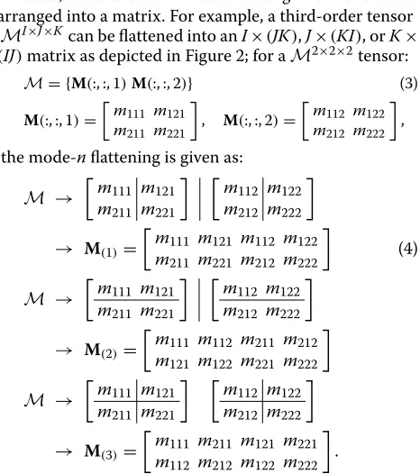
That is, all the column vectors along the mode n are arranged into a matrix. For example, a third-order tensor

MI×J×K _{can be ﬂattened into an}_I_×₍_JK₎_,_J_×₍_KI₎_{, or}_K_×

(IJ)matrix as depicted in Figure 2; for aM2×2×2tensor: M= {M(:, :, 1)M(:, :, 2)} (3)

M(:, :, 1)=

m111 m121

m211 m221

, M(:, :, 2)=

m112 m122

m212 m222

,

the mode-nﬂattening is given as:

M →

m111 m121

m211 m221

m112 m122

m212 m222

→ M(1)=

m111 m121 m112 m122

m211 m221 m212 m222

(4)

M →

m111 m121

m211 m221

m112 m122

m212 m222

→ M(2)=

m111 m112 m211 m212

m121 m122 m221 m222

M →

m111 m121

m211 m221

m112 m122

m212 m222

→ M(3)=

m111 m211 m121 m221

m112 m212 m122 m222

.

The operation of the mode-nﬂattening will be denoted as matn(·), i.e., matn(M)=M(n).

(3)

Figure 2Mode-nﬂattening of a third-order tensor.

Multiplication of a tensor and a matrix is performed by n-mode product; then-mode product of a tensorWwith a matrixUis denoted as

M=W×nU (5)

and is carried out by matrix multiplication in terms of ﬂattened matrices:

M(n)=U W(n) (6)

or elementwise

W×nU

i1...in−1jin+1...iN = In

in=1

wi1i2...iNujin (7)

wherewandudenote the elements ofW andU, respec-tively. IfW ∈ RI1×I2×···×IN _and_UT ∈ RKn×In_{, then the}

dimension ofW ×nUT becomesI1×I2× · · · ×In−1×

Kn×In+1× · · · ×IN.

As an extension of singular value decomposition (SVD) to tensor objects, Tucker decomposition decomposes a tensor as follows [4]:

MI1×I2×···×IN WK1×K2×···×KN N

n=1

×nUn (8)

whereUn∈RIn×Kn,Kn≤In(n=1,. . .,N). The core ten-sorWand mode matricesUn’s correspond to the matrices of singular values and orthonormal basis vectors in matrix SVD, respectively. An example of Tucker decomposition of a third-order tensor is illustrated in Figure 3.

The core tensorW and mode matricesUn’s in Tucker decomposition can be computed such that they minimize

Error=M−W N

n=1

×nUn

2 (9)

where the norm of a tensor is deﬁned as X = I1

i1=1

I2

i2=1. . .

IN iN=1x

2

i1i2...iN. A representative

tech-nique for Tucker decomposition is the alternating least

Figure 3Tucker decomposition of a third-order tensor.

squares (ALS) [12]; the basic idea is to compute each mode matrixUnalternatingly with other mode matrices ﬁxed. For more details on Tucker decomposition, refer to [4]. In the following section, we explain probabilistic 2-mode analysis in the context of speaker adaptation.

2.2 Speaker adaptation using Tucker decomposition

The probabilistic 2-mode analysis based method is a prob-abilistic extension of the Tucker decomposition based method. Thus, we compare the probabilistic approach with the Tucker decomposition based method in the experiments. In this section, we explain the speaker adap-tation based on the Tucker decomposition of training models in [5]. In this article, speaker adaptation is per-formed by updating the mean vectors of the output dis-tribution of an HMM. The HMM mean vectors of each training speaker are arranged in anR×Dmatrix:

Ms=

μ

μμ_s_;1. . . μμμ_s_;_r. . . μμμ_s_;_RT, s=1,. . .,S. (10)

Here,μμμ_s_;_rdenotes the mean vector corresponding to mix-turerof thesth training speaker model.

All the centered HMM mean vectors of training speak-ers,Ms−M

S

s=1whereM=1/S

sMs, are collectively expressed as a third-order tensorM, and we decompose the training tensor by Tucker decomposition as follows:

MR×D×S_GKR×KD×KS×

1Umixture×2Udim×3Uspeaker (11)

=GKR×KD×KS×

3Uspeaker×1Umixture×2Udim.

In the above equation,Umixture∈RR×KR,Udim∈RD×KD, andUspeaker ∈ RS×KS are basis matrices for the mixture component, dimension of the mean vector, and training speaker, respectively (KR ≤ R− 1,KD ≤ D−1, and KS ≤ S −1); the core tensor G is common across the mixture component, dimension of the mean vector, and training speaker. In Equation (11), thesth row vector of

Uspeaker, which is denoted as uspeaker;s, corresponds to the speaker weight of thesth speaker, thus the low-rank approximation of thesth speaker model is given by

Ms

GKR×KD×KS×

3uspeaker;s

(4)

If we deﬁne the augmented speaker weight WKR×KD

s ≡

GKR×KD×KS×

3uspeaker;s, Equation (12) becomes

MsWs×1Umixture×2Udim+M (13)

=UmixtureWsUTdim+M.

Thus, we express the model of a new speaker as

Mnew =UmixtureWnewUTdim+M. (14)

For the given adaptation dataO= {o1,. . .,oT}, we derive the equation for ﬁnding the speaker weight in a maximum likelihood (ML) criterion:

t

r

γr(t)Cr−1UdimWTnew

≡WT

new,aug

uT_mixture;_rumixture;r (15)

=

t

r

γr(t)C−r1

ot−mTr

umixture;r

whereγ_r(t)denotes the occupation probability of being at mixturerattgivenO,Crthe covariance matrix of therth Gaussian component of an SI HMM (in this article, a diag-onal covariance matrix is used);umixture;r andmr denote therth row vectors ofUmixtureandM, respectively. In the above equation,Wnew, augcan be computed using a tech-nique similar to MLLR adaptation and the weight of the new speaker is obtained by

ˆ

Wnew=Wnew, augUdim (16)

which is plugged into Equation (14) to produce the model updated for the new speaker.

2.3 Probabilistic 2-mode analysis

The advantage of probabilistic 2-mode analysis over Tucker decomposition is similar to that of PPCA over standard PCA; probabilistic 2-mode analysis can deal with missing entries in the data tensor (although this is not the case in our experiments). In the modeling perspec-tive, probabilistic 2-mode analysis assumes a distribution of latent variables, thus it is suitable for a MAP framework. In this section, the ensemble of training models is expressed as

M= {Ms}Ss=1. (17)

Assuming the HMM mean vectors of training speakers are drawn from the matrix-variate normal distribution [13], we derive the adaptation equation based on the probabilistic 2-mode analysis of training models. We use probabilistic 2-mode analysis, the second-order case of PTA [8], to decompose the training models expressed in matrix form. The latent tensor model is expressed as

M=W

N

n=1

×nUn+Mmean+E (18)

whereWdenotes the latent tensor,Un’s the factor loading matrices,Mmeanthe mean, andEis the error/noise pro-cess. The 2-mode case of the latent tensor model is given by

M=W×1U1×2U2+Mmean+E (19)

which becomes, for the training models{M1,. . .,MS},

Ms=Ws×1U1×2U2+Mmean+Es (20)

=UmixtureWsUTdim+Mmean+Es

whereWs∈RKR×KD denotes the latent matrix,Umixture∈

RR×KR _and _U

dim ∈ RD×KD the factor loading matrices (KR ≤ R−1 and KD ≤ D−1),Mmean the mean, and

Es the error/noise process. (Mode matrices and dimen-sions are deﬁned as follows:U1 = Umixture,U2 = Udim,

I1 = R,I2 = D,K1 = KR, andK2 = KD.) The distribu-tion ofWsis assumed to be a matrix-variate normal, i.e.,

Ws ∼ N(0KR×KD,IKR ⊗IKD)where⊗denotes the

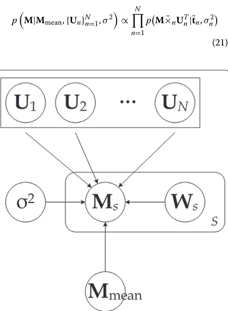
Kro-necker product, and independent of Es whose elements followN(0,σ2). Figure 4 shows the graphical model rep-resenting the probabilistic 2-mode model.

In Equation (20), it is computationally intractable to cal-culate Un’s simultaneously. So, the following decoupled predictive density is deﬁned:

pM|Mmean,{Un}Nn=1,σ2

∝

N

n=1

pM¯×nUTn|¯tn,σn2

(21)

(5)

where ¯tn ∈ RIn×1 andσn2 denote the mean vector and noise variance, respectively, for moden;M¯×nUTn ≡M×1

UT₁. . .×n−1UT_n₋₁×n+1UT_n₊₁. . .×N UT_N, i.e., the prod-uct ofMwith all the mode matrices except moden, which is called the contractedn-mode product [14]. That is, the nth probabilistic function is deﬁned as the projectedMby allUj’s expectUn. Given observed dataM, the decoupled posterior probabilistic function is deﬁned as

pMmean,{Un}Nn=1,σ2|M

∝ N

n=1

p¯tn,Un,σn2,M,{Uj}Nj=1,j=n

.

(22)

By Bayes’ theorem, thenth posterior distribution can be expressed in terms of the decoupled likelihood function and the decoupled prior distribution:

p¯tn,Un,σn2,M,{Uj}Nj=1,j=n

∝

pM,{Uj}Nj=1,j=n|¯tn,Un,σn2

p¯tn,Un,σn2

. (23)

Therefore, the decoupled predictive density is given by

p(M|M)∝p

M|Mnew,{Un}Nn=1,σ2

×pMmean,{Un}Nn=1,σ2|M

(24)

=

N

n=1

p

M¯×nUTn|¯tn,σn2

×pM,{Uj}Nj=1,j=n|¯tn,Un,σn2

.

pt¯n,Un,σn2

is dropped out for a ﬁxedUn). This is the 2-mode case of the PTA in [8]. In our case, Equation (24) is given by

p(M|M)∝p

UT_dimMT|¯tmixture,σmixture2

×pM,Udim|¯tmixture,Umixture,σmixture2

(25)

×pUT_mixtureM|¯tdim,σ_dim2

×pM,Umixture|¯tdim,Udim,σdim2

.

Now,Un’s are obtained by maximizing the following pos-terior distribution:

p{Un}Nn=1|M

≈

N

n=1

pUn|M¯×nUTn

(26)

where pUn|M¯×nUTn

≡ S

s=1Ms¯×nUTn. The expectation-maximization (EM) algorithm [15] is applied to computeUn’s. The application of the EM algorithm to construct probabilistic 2-mode model is explained in the next section.

2.4 Construction of probabilistic 2-mode model for speaker adaptation

In Equation (20), for the given training models, the maxi-mum likelihood (ML) estimate ofMmeanis given asM=

(1/S)_sMs and {Un,σn2} can be estimated as follows.

First, let us deﬁne the followings: Lettn;j ∈ RIn×1be the jth column vector of

T(n)=matnM¯×nUTn

(27)

for 1≤j≤ ¯InS(I¯n =Nj=1,j=nIj) andxn;j ∈RKn×1be the jth column vector of

X(n)=matn

M

N

n=1

×nUTn

. (28)

Let us suppose tn|xn ∼ N(Unxn + ¯tn,σn2IIn) and xn ∼ N(0Kn×1,IKn). Then, by integrating outxn, tn ∼ N(¯tn,Gn)wheret¯n=1/(¯InS)j¯I=nS1tn;jandGn=UnUTn+

σ_n2IIn. Consequently,

xn|tn∼N

H−_n1UT_n(tn− ¯tn),σn2H−n1

(29)

where Hn = UTnUn + σn2IKn. The right-hand side

of Equation (26) becomes

logpUn|M¯×nUTn

∝ −I¯nS 2

log|Gn| +trG−n1Sn

(30)

whereSn = 1/(¯InS−1)¯Ij=nS1

tn;j− ¯tn

T and tr[·] denotes the trace of a matrix. Summing up for all the modes, we obtain the following log-likelihood function of the posterior distribution:

L=

n

logpUn|M¯×nUn

∝ − n _¯ InS 2

log|Gn| +tr

G−_n1Sn

. (31)

The graphical model representation of the decoupled probabilistic model is shown in Figure 5.

We seek to ﬁndUn’s that maximize the log-likelihood function alternatingly. Mode matricesU1andU2are ini-tialized with the results from the Tucker decomposition which minimizes the reconstruction error:

Error= s

Ms−

Ws×1U1×2U2+M 2

. (32)

With the initial U1 and U2, the following procedure is performed for each mode (n=1, 2).

Each training model is projected into mode matrices except modenand expressed in a mode-nmatrix:

Ts,(n)=matn

Ms¯×nUTn

. (33)

All the column vectors ofTs,(n)

S

s=1constitute the train-ing data set:

{tn;j}, 1≤j≤ ¯InS. (34)

(6)

E-step: From Equation (31), the expectation of the log-likelihood function of complete data w.r.t. pxn;j|tn;j,¯tn,Un,σn2

is given as

Lc =

n

s

Elogp(Ms,Ws|{U}Nj=1,j=n)

(35)

=

n InS

j=1

Elogp(tn;j,xn;j|{U}Nj=1,j=n)

where

logp(tn;j,xn;j|{U}Nj=1,j=n)=logp(xn;j)+logp(tn;j|xn;j)

(36)

∝ −xn;j2− In

2 log(σ 2

n)

− 1

σ2

n

tn;j−Unxn;j− ¯tn2.

So,

Lc ∝ −

n ¯ InS

j=1

trxn;jxTn;j

+ 1

σ2

n

(tn;j− ¯tn)T(tn;j− ¯tn) (37)

+In 2 log(σ

2

n)+ 1

σ2

n

trUT_nUnxn;jxTn;j

− 2

σ2

n

xn;jTUnT(tn;j− ¯tn)

Figure 5Graphical model representation of the decoupled probabilistic model.

with the suﬃcient statistics are given as follows from Equation (29):

xn;j =H−n1UTn

tn;j− ¯tn

(38)

xn;jxTn;j =σn2Hn−1+ xn;jxn;jT.

M-step: Model parameters are updated by maximizing

Lcw.r.t.Unandσn2. Setting∂UnLc =0 produces

Un=

I¯nS

j=1

tn;j− ¯tn

xn;jT

¯InS

j=1

xn;jxTn;j

−1 . (39)

Next, setting∂_σ2

nLc =0 produces

σ_n2= 1

In¯InS ¯ InS

j=1

tn;j− ¯tn2−2xn;jTUTn

tn;j− ¯tn

+trxn;jxTn;jUTnUn

.

(40)

Essentially, the procedure applies PPCA to the data set

{tn;j}for each mode.

2.5 Estimation of prior distribution

Given model parameters {M,Un,σn2}, the weight matrix for the training speaker modelMsis obtained by

Ws=

Ms−M

2

n=1

×n

H−_n1UT_n (41)

=H−₁1UT_mixtureMs−MH−₂1UT_dimT.

From the set of weight matrices {Ws}Ss=1, the distribu-tion of the weight is estimated. In deriving the adaptadistribu-tion equation in the MAP framework, the parameters for the prior distribution can be obtained in closed-form solu-tions if p(W) follows a conjugate distribution. Hence, we assume the prior distribution of the weight to be a matrix-variate normal:

p(W)∝ 1

||KD/2||KR/2

exp

−1

2tr

(W−Wmean)T−1(W−Wmean)−1

.

(42)

(7)

is assumed to be the identity matrix [17], and the hyperparameters are estimated as:

Wmean= 1 S

s

Ws=0KR×KD (43)

= 1

S−1

s

WsWTs.

2.6 Speaker adaptation in the MAP framework

Based on Equation (20), we express the model of a new speaker as

Mnew=UmixtureWnewUTdim+M. (44)

For the given adaptation data O = {o1,. . .,oT}, we estimate the adaptation parameter in a MAP criterion:

MAP=arg max

p(|O) (45)

∝arg max

p(O|)p()

∝arg max

logp(O|)+logp()

where= {Wnew}denotes the model parameter.

Using the EM algorithm, we obtain the following auxil-iaryQ-function to be optimized (discarding the terms that are independent of the model parameter):

Q(,)ˆ =−1 2

t

r

γr(t)tr(ot−mTnew;r)TC−r1(ot−mTnew;r)

(46)

−₂1tr(WnewUdim)T−1(WnewUdim)

where and ˆ denote the current and updated model parameters, respectively, and mnew;r =

umixture;rWnewUTdim +mr. In ﬁnding the speaker weight, we computeWnew, aug ≡ WnewUdim, from whichWnew is obtained. Solving in this way, we can use the row-by-row technique in MLLR adaptation [6]. Setting

∂WnewQ(,)ˆ =0 yields the following equation:

t

r

γr(t)C−r1UdimWTnew

≡WT

new, aug

uT_mixture;rumixture;r+UdimWTnew

≡WT

new, aug

−1

(47)

=

t

r

γr(t)C−r1

ot−mTr

umixture;r.

The above equation can be solved for Wnew, aug in a similar way to MLLR adaptation in [6]: we deﬁne the followings:

Vr=

t

γr(t)C−r1 (48)

Dr=uTmixture;rumixture;r

G(i)=

r

vr(i,i)Dr

Z=

t

r

γr(t)C−r1

ot−mTr

umixture;r

(i)=

1 S−1

s

ws;iwTs;i

wherevr(i,i)denotes the(i,i)element ofVr andws;ithe ith column vector ofWs, aug≡WsUdim. Then, the speaker weight can be computed:

wT_{new, aug,}₍_i₎=

G(i)+−(i)1

−1

zT₍_i₎, i=1,. . .,D (49)

where wnew, aug,(i) denotes the ith row of Wnew, aug and

z(i)theith row vector ofZ. The method becomes similar

to MAPLR adaptation in [11]. Finally, the speaker weight is obtained as

ˆ

Wnew=Wnew, augU+_dim (50)

where [·]+ denotes the pseudoinverse of a matrix. The weight is plugged into Equation (44) to produce the model adapted to the new speaker.

2.7 Speaker adaptation techniques compared in the experiments

In this section, we brieﬂy review the speaker adapta-tion techniques compared with the probabilistic 2-mode analysis based method: eigenvoice adaptation [3], MLLR adaptation [6], and MAPLR adaptation [11].

In eigenvoice adaptation, the collection of HMM mean vectors of speakersis arranged in an(RD)×1 vector:

μ μ μs=

⎡ ⎢ ⎢ ⎢ ⎣

μμμs;1

μμμs;2 .. .

μ μ μs;R

⎤ ⎥ ⎥ ⎥

⎦. (51)

Then, the set of Ssupervectors, {μμμ1,. . .,μμμS}, is decom-posed by PCA to produce the adaptation model

μ μ

μnew =wnew+ ¯μμμ (52)

(8)

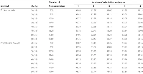
Table 2 Word recognition accuracy (%) of the Tucker 3-mode and probabilistic 2-mode based methods

Number of Number of adaptation sentences

Method (KR,KD) free parameters 1 2 3 4 5

Tucker 3-mode (20, 35) 700 91.84 92.98 93.07 92.99 93.11 (20, 38) 760 91.82 92.83 93.11 93.01 93.01 (30, 35) 1050 90.77 92.99 93.18 93.09 92.94 (30, 38) 1140 90.77 92.86 93.18 93.01 92.86 (40, 35) 1400 89.39 92.85 93.11 93.24 93.03 (40, 38) 1520 89.16 92.77 93.20 93.14 92.98 (50, 35) 1750 87.95 92.34 93.24 93.26 93.13 (50, 38) 1900 87.75 92.47 93.27 93.31 93.16 Probabilistic 2-mode (20, 35) 700 93.07 93.18 93.26 93.27 93.16 (20, 38) 760 92.96 93.07 93.03 93.24 93.13 (30, 35) 1050 92.98 93.20 93.24 93.24 93.31 (30, 38) 1140 92.94 93.33 93.33 93.27 93.31 (40, 35) 1400 93.13 93.20 93.39 93.24 93.01 (40, 38) 1520 93.14 93.22 93.33 93.20 93.24 (50, 35) 1750 93.26 93.35 93.37 93.29 93.29 (50, 38) 1900 93.37 93.44 93.42 93.31 93.39

The number of mixture componentsR=3472·8and the dimension of acoustic feature vectorD=39. The number of free parameters isKR×KD. TheK×1 weight vector can be obtained by maximizing

the likelihood of the adaptation data, which is given by

ˆ wnew=

t

r

γr(t) rTC−r1r

−1

×

t

r

γr(t) TrC−r1

ot− ¯μμμr

(53)

whererandμμμ¯rdenote theD×Ksubmatrix andD×1 subvector corresponding to therth mixture ofandμμμ¯, respectively.

In MLLR adaptation, the updated model for a new speaker is obtained by linearly transforming the SI model (assuming a global regression matrix):

μ

μμnew,r =Wnewξξξr, ξξξr=

ω μ μ μSI,r

(54)

whereμμμSI,rdenotes the mean vector of the SI HMM cor-responding to mixturerandωis the bias oﬀset term:ω=

1 to include the term andω=0 otherwise (ω= 1 in our experiments). TheD×(D+1)transformation matrix can be obtained in an ML criterion, which yields the following equation:

t

r

γr(t)C−r1otξξξTr (55)

=

t

r

γ_r(t)C_r−1WnewξξξrξξξTr.

The above equation can be solved forWnew:

ˆ

wT_new,₍_i₎=G−₍_i₎1zT₍_i₎, i=1,. . .,D (56)

wherewˆnew,(i)andz(i)denote theith row vectors ofWˆnew andZ, respectively;G(i)andZare deﬁned as:

Vr=

t

γr(t)C−r1 (57)

Dr=ξξξrξξξTr

G(i)=

r

vr(i,i)Dr

Z=

t

r

γr(t)C−r1otξξξTr

wherevr(i,i)denotes the(i,i)element ofVr.

In MAPLR adaptation, the prior for the transformation matrix is used in the MLLR framework. The parameters for the prior are obtained from the MLLR transformation matrices of training speakers{W1,. . .,WS}:

¯ w(i)=

1 S

s

ws,(i) (58)

(i)=

1 S−1

s

ws,(i)− ¯w(i)

T

ws,(i)− ¯w(i)

(9)

Table 3p-values from the matched-pairt-test

Methods Number of adaptation sentences

1 2 3 4 5

Prob. 2-mode and Tucker 3-mode <0.01 0.22 0.08 0.03 0.34 Prob. 2-mode and MAPLR 0.10 <0.01 <0.01 0.01 0.02 Prob. 2-mode and MLLR, block-diagonal <0.01 0.01 0.04 <0.01 0.05 Prob. 2-mode and EV <0.01

Tucker 3-mode and MLLR, block-diagonal 0.43 0.18 0.63 0.17 0.22 Tucker 3-mode and EV 0.94 <0.01 <0.01 <0.01 <0.01

For the probabilistic 2-mode and Tucker 3-mode based models,KR=20andKD=35. MAP criterion. Deriving the equation in the same way as above, we can obtain the following:

ˆ

wT_new,₍_i₎=

G(i)+−(i)1

−1

z(i)+ ¯w(i)−(i)1

T

. (59)

3 Experiments

We carried out the large-vocabulary continuous-speech recognition (LVCSR) experiments using the Wall Street Journal corpus WSJ0 [18]. In building the SI model, we used 12754 utterances of 101 speakers from the corpus. As the acoustic feature vector, we used the 39-dimensional vector consisting of 13-dimensional mel-frequency cep-stral coefficients (MFCCs) including the 0th cepcep-stral coef-ficient, their derivative coefficients, and their acceleration coefficients. The feature vector was extracted with the 20-ms Hamming window with the frame sliding of 10 20-ms. Using the HMM toolkit (HTK) [19], we built a tied-state triphone model (word-internal triphones) with 3472 tied states and 8-mixture Gaussian.

To build training models for constructing bases, we transformed the SI model by MLLR adaptation [6] using 32 regression classes followed by maximum a posteriori (MAP) adaptation [10]. We used the 101 adapted mod-els to build the Tucker decomposition and probabilistic tensor based models as well as eigenvoice.

For adaptation and recognition test, we used Nov’92 5K non-verbalized adaptation and test sets. The num-ber of testing speakers was 8; adaptation set was used for adaptation and testing set of 330 sentences was used for recognition test (the number of testing utterances per speaker was about 40). The length of an adaptation sen-tence was about 6 s and the adaptation was performed in supervised mode. In recognition test, we used WSJ 5K non-verbalized 5k closed-vocabulary set and WSJ stan-dard 5K non-verbalized closed bigram.

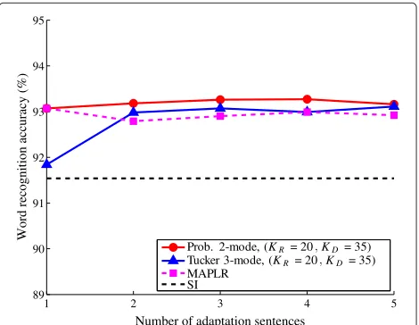
The word recognition accuracy of the SI model is 91.54%. Table 2 shows the results of the Tucker decom-position and probabilistic 2-mode based methods (KS = 100 in the Tucker decomposition based model). In the table, the probabilistic 2-mode based method shows improved performance over the Tucker decomposition

based method for small amounts of adaptation data, which can be evidently seen in Figure 6 for the Tucker decomposition and probabilistic 2-mode based models with (KR = 20,KD = 35). The results of MAPLR [11] are also shown in the figure. The use of MAP framework contributes to improved performance for small amounts of adaptation data. The number of free parameters of each method is given as follows: 20·35 for the Tucker 3-mode and probabilistic 2-3-mode based 3-models, and 39·40 for MAPLR adaptation. In Figure 7, the Tucker decom-position based method is compared with MLLR and eigenvoice adaptation techniques. The figure shows that the Tucker decomposition based method outperforms MLLR and eigenvoice adaptation techniques for adapta-tion sentences>1. It can be inferred from the figure that eigenvoice adaptation will outperform the Tucker decom-position based method or MLLR for sparse adaptation data. Thep-values from the matched-pairt-test are shown in Table 3; although the values are not always small, the performance improvement of the probabilistic 2-mode based method seems meaningful. Additionally, Figure 8

1 2 3 4 5

89 90 91 92 93 94 95

Number of adaptation sentences

Word recognition accuracy (%)

Prob. 2-mode, (KR= 20 KD = 35)

Tucker 3-mode, (KR = 20 KD= 35)

MAPLR SI

(10)

1 2 3 4 5 89

90 91 92 93 94 95

Tucker 3-mode, (KR = 20 KD= 35)

MLLR, block-diagonal

Eigenvoice,K = 50

Figure 7Word recognition accuracy of the Tucker 3-mode based model, MLLR, and eigenvoice adaptation.

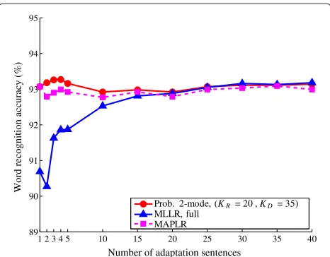
shows the performance of the probabilistic 2-mode based model with (KR=20,KD=35), MLLR adaptation with a full regression matrix, and MAPLR adaptation for adapta-tion data of about 6–240 s; for adaptaadapta-tion sentences≥10 (about 60 s), the probabilistic 2-mode based model shows the comparable performance with MLLR adaptation and MAPLR adaptation. In Figure 8, the p-values are given as: p < 0.01 for 1–5 adaptation sentences between the probabilistic 2-mode based model and MLLR adaptation, p<0.05 for 2–5 adaptation sentences between the proba-bilistic 2-mode based model and MAPLR adaptation. The number of free parameters of each method is summarized in Table 4.

We think that the performance improvement of the pro-posed method over MLLR or MAPLR adaptation comes

1 2 3 4 5 10 15 20 25 30 35 40 89

90 91 92 93 94 95

Prob. 2-mode, (KR= 20 ,KD= 35)

MLLR, full MAPLR

Figure 8Word recognition accuracy of the probabilistic 2-mode based model, MLLR, and MAPLR adaptation.

Table 4 Number of free parameters of adaptation techniques

Method Number of free parameters

Probabilistic 2-mode based model 20·35(KR·KD)

Tucker 3-mode based model 20·35(KR·KD)

MLLR, 3-block-diagonal regression matrix 13·40 MLLR, full regression matrix 39·40 MAPLR adaptation 39·40 Eigenvoice 50

from the use of basis vectors and speaker weight of large dimension. Additionally, we think that the performance improvement of the probabilistic 2-mode based method in the MAP framework over the Tucker decomposition based method in the ML framework for small amounts of adaptation data (e.g., 1 adaptation sentence) is due to its constraint on the weight. If the amount of adaptation data is small (e.g., 1 adaptation sentence), the weight can-not be reliably estimated in the ML framework where the weight is estimated using only adaptation data without constraint, as done in the Tucker decomposition based method. The results conﬁrm that constraint on the weight in the MAP framework can produce better model when the amount of adaptation data is small.

The selection of appropriate dimensions of model parameters (e.g.,KRandKD) in the probabilistic 2-mode analysis depends on the training models and also available adaptation data. The selection of model parameters aﬀects the performance of the system, but how to choose the optimum model parameters is not obvious, which needs a further study.

4 Conclusions

In this article, we applied probabilistic tensor analysis to the adaptation of HMM mean vectors to a new speaker. The training models consisted of the mean vectors of HMMs expressed in matrix form and the training set was decomposed by probabilistic 2-mode analysis. The prior distribution of the adaptation parameter was estimated from the training models. Then, the speaker adaptation equation was derived in the MAP framework. Compared with the speaker adaptation method based on Tucker 3-mode decomposition in the ML framework, the pro-posed method further improved the performance for small amounts of adaptation data.

Abbreviations

ALS: Alternating Least Squares; ASR: Automatic Speech Recognition; EM: Expectation-Maximization; HMM: Hidden Markov Model; HTK: HMM Toolkit; LVCSR: Large-Vocabulary Continuous-Speech Recognition; MAP: MaximumA

Posteriori; MAPLR: MaximumA PosterioriLinear Regression; MFCC:

(11)

Analysis; SD: Speaker-Dependent; SI: Speaker-Independent; SVD: Singular Value Decomposition; WSJ: Wall Street Journal.

Competing interests

The author declares that they have no competing interests.

Received: 29 May 2012 Accepted: 13 March 2013 Published: 11 April 2013

References

1. LR Rabiner, A tutorial on hidden Markov models and selected applications in speech recognition. Proc. IEEE.77(2), 257–286 (1989)

2. M Gales, S Young, The application of hidden Markov models in speech recognition. Found. Trends Signal, Process.1(3), 195–304 (2008) 3. R Kuhn, J-C Junqua, P Nguyen, N Niedzielski, Rapid speaker adaptation in

eigenvoice space. IEEE Trans. Speech Audio Process.8(6), 695–707 (2000) 4. TG Kolda, BW Bader, Tensor decompositions and applications. SIAM Rev.

51(3), 455–500 (2009)

5. Y Jeong, inProceedings of IEEE International Conference on Acoustics,

Speech, and Signal Processing. Speaker adaptation based on the

multilinear decomposition of training speaker models (Dallas, TX, 2010), pp. 4870–4873

6. CJ Leggetter, PC Woodland, Maximum likelihood linear regression for speaker adaptation of continuous density hidden Markov models. Comput. Speech Lang.9(2), 171–185 (1995)

7. Y Jeong, Acoustic model adaptation based on tensor analysis of training models. IEEE Signal Process. Lett.18(6), 347–350 (2011)

8. D Tao, M Song, X Li, J Shen, J Sun, X Wu, C Faloutsos, SJ Maybank, Bayesian tensor approach for 3-D face modeling. IEEE Trans. Circ. Syst. Video Technol.18(10), 1397–1410 (2008)

9. ME Tipping, CM Bishop, Probabilistic principal component analysis. J. R. Stat. Soc. Ser. B-Stat. Methodol.61(3), 611–622 (1999)

10. J-L Gauvain, C-H Lee, Maximuma posterioriestimation for multivariate Gaussian mixture observations of Markov chains. IEEE Trans. Speech Audio Process.2(2), 291–298 (1994)

11. C Chesta, O Siohan, C-H Lee, inProceedings of EUROSPEECH, vol. 1. Maximuma posteriorilinear regression for hidden Markov model adaptation (Budapest, Hungary, 1999), pp. 211–214

12. JD Carroll, JJ Chang, Analysis of individual diﬀerences in multidimensional scaling via an N-way generalization of “Eckart-Young” decomposition. Psychometrika.35(3), 283–319 (1970)

13. AK Gupta, DK Nagar,Matrix Variate Distributions. (Chapman and Hall/CRC, Boca Raton, FL, 1999)

14. BW Bader, TG Kolda, Algorithm 862: MATLAB tensor classes for fast algorithm prototyping. ACM Trans. Math. Softw.32(4), 635–653 (2006) 15. AP Dempster, NM Laird, DB Rubin, Maximum likelihood from incomplete

data via the EM algorithm. J. R. Stat. Soc. Ser. B-Stat. Methodol.39(1), 1–38 (1977)

16. AK Gupta, T Varga,Elliptically Contoured Models in Statistics. (Kluwer, Norwell, MA, 1993)

17. O Siohan, C Chesta, C-H Lee, Joint maximum a posteriori adaptation of transformation and HMM parameters. IEEE Trans. Speech Audio Process.

9(14), 417–428 (2001)

18. DB Paul, JM Baker, inProceedings of DARPA Speech and Natural Language

Workshop. The design for the Wall Street Journal-based CSR corpus

(Austin, TX, 1992), pp. 357–362

19. S Young, G Evermann, D Kershaw, G Moore, J Odell, D Ollason, D Povey, V Valtchev, P Woodland,The HTK Book, Version 3.2. (Cambridge University Engineering Department, England, 2002)

doi:10.1186/1687-4722-2013-7

Cite this article as:Jeong:Speaker adaptation in the maximuma posteriori framework based on the probabilistic 2-mode analysis of training models.

EURASIP Journal on Audio, Speech, and Music Processing20132013:7.