The Thirty-Third AAAI Conference on Artificial Intelligence (AAAI-19)
Bounded Suboptimal Search with Learned Heuristics for Multi-Agent Systems
Markus Spies,
∗Marco Todescato,
∗Hannes Becker, Patrick Kesper, Nicolai Waniek, Meng Guo
Bosch Center for Artificial Intelligence (BCAI), Renningen, Germany{markus.spies2, marco.todescato, hannes.becker, patrick.kesper, nicolai.waniek, meng.guo2}@de.bosch.com
(*) equal contribution
Abstract
A wide range of discrete planning problems can be solved optimally using graph search algorithms. However, optimal search quickly becomes infeasible with increased complexity of a problem. In such a case, heuristics that guide the plan-ning process towards the goal state can increase performance considerably. Unfortunately, heuristics are often unavailable or need manual and time-consuming engineering. Building upon recent results on applying deep learning to learn gen-eralized reactive policies, we propose to learn heuristics by
imitation learning. After learning heuristics based on optimal examples, they are used to guide a classical search algorithm to solve unseen tasks. However, directly applying learned heuristics in search algorithms such as A∗ breaks optimal-ity guarantees, since learned heuristics are not necessarily ad-missible. Therefore, we (i) propose a novel method that uti-lizes learned heuristics to guide Focal Search A∗, a variant of A∗with guarantees on bounded suboptimality; (ii) compare the complexity and performance of jointly learning individual policies for multiple robots with an approach that learns one policy for all robots; (iii) thoroughly examine how learned policies generalize to previously unseen environments and demonstrate considerably improved performance in a simu-lated complex dynamic coverage problem.
1
Introduction
Intelligent robotic systems have to select from a diverse set of actions to perform complex operations. For instance, they must plan sequences of optimal actions to complete specified tasks such as following trajectories, navigation within clustered workspace, or coordination among different robots. Unfortunately, planning is known to be a hard com-putational problem that often relies on heavily engineered solutions, for instance heuristic-based rules which are tai-lored to specific environments (Ghallab, Nau, and Traverso 2004; LaValle 2006; Latombe 2012). These solutions typi-cally lack generalization capabilities and performance guar-antees for new environments. Conversely,intelligentrobotic systems will be deployed in previously unseen, complex en-vironments and thus need capabilities to plan dynamically while reacting to unforeseen situations.
Here, we propose a step towards bridging this gap by ex-ploiting recent advancements in deep learning which yields
Copyright © 2019, Association for the Advancement of Artificial Intelligence (www.aaai.org). All rights reserved.
intelligent behavior without hand-crafted solutions. Specifi-cally, rather than synthesizing an entire plan, we learn poli-cies that output action probabilities given an observation of the current system state. We build upon recent results where a reactive policy was learned from expert demonstrations us-ing a deep neural network (Groshev et al. 2017). The learned policy generalizes to some degree to novel environments, which is, however, limited and typically not optimal for ev-ery situation. Nevertheless the learned policy can be used as aguiding heuristicin classical planners such as A∗. Still, di-rectly applying learned policies, as previously proposed by Groshev et al. (2017), breaks optimality or even complete-ness guarantees, because the learned heuristic is not ensured to be admissible (Russell and Norvig 2016).
In this paper, we therefore present a novel combination of learned policies withω-optimal A∗focal search (A∗ω),
in-troduced by Pearl and Kim (1982). Our algorithm exploits guidance from learned policies and ensures not only com-pleteness but also bounds on suboptimality. We model the generalized policy with a deep convolutional neural network that takes observations of the environment states as input and outputs next actions as well as the predicted remaining plan length. Furthermore, we propose two different heuristics that are derived from the outputs of the learned network, one that directly predicts a value function, and a second one that esti-mates the path likelihood of nodes that are expanded during search.
In summary, the contibution of this paper is (i) we propose a novel combination of learned heuristics with A∗ω search. This combination guarantees bounds on suboptimality while exploiting guidance from learned policies; (ii) we present a general framework for learning control policies and extend previous work to multi-agent systems; (iii) we introduce a novel problem domain based on the real world application of autonomous valet parking. Extensive experimental evalu-ations demonstrate the advances or our approach over exist-ing methods in this domain.
2
Related work
commonly made between solution quality and planning effi-ciency. For instance, A∗ variants with bounded relaxation have been proposed that allow suboptimal results (Arya et al. 2004; Helmert and Domshlak 2009; Pearl and Kim 1982; Cohen et al. 2018). In particular, A∗ω by Pearl and
Kim (1982) uses an additional heuristichF(n)that does not
need to be admissible but guides planning into promising re-gions. Cohen et al. (2018) present ananytime-version of A∗ω
that tightens the bound iteratively over the planning time. Finding good heuristics can be hard and in many cases in-volves tedious manual work. Moreover, good heuristics are often subject to the environments for which they were de-signed, i.e., they do not generalize well to novel environ-ments. Consequently, machine learning has been suggested and successfully applied to learn and improve such heuris-tics. For instance, Samadi, Felner, and Schaeffer (2008) combine several existing heuristics using artificial neural networks and Arfaee, Zilles, and Holte (2011) propose the method of iterative deepening, which starts planning with weak heuristics and iteratively improves them. In contrast, we focus on the combination of bounded suboptimal plan-ning with learned policies.
Over the past years, deep neural networks (DNN) have been used with extraordinary success in a plethora of different domains, e.g., image classification (Krizhevsky, Sutskever, and Hinton 2012), natural language processing (Sutskever, Vinyals, and Le 2014), or control (Mnih et al. 2015). This, together with DNNs theoretically being univer-sal function approximators (Cybenko 1989), has motivated their usage in the planning domain. One of the first examples is the work by Ernandes and Gori (2004), in which DNNs were used to learn heuristic value functions for guided plan-ning. Whereas they apply likely admissible heuristics for which the admissibility requirement is relaxed in a proba-bilistic sense, our method computes solutions with a hard suboptimality bound.
Besides learning value functions as heuristics, Groshev et al. (2017) proposes to directly learn policies, i.e., map-pings from state to actions by imitation learning. Imitation learning and, in particular, behavioral cloning are supervised learning techniques in which a model learns the correct con-trol policy based on sequences of observation-action pairs that are provided by an expert demonstrator. As shown in Groshev et al. (2017), the learned policy is able to general-ize to situations it has never seen during training. Behavioral cloning was also successfully used in applications such as path following with obstacle avoidance (Tamar et al. 2016) or focused robot skills (M¨ulling et al. 2013). Others used actor-critic methods to directly learn policies in multi-agent scenarios for the purpose of collective construction (Sar-toretti et al. 2018).
Our approach is closely related and builds upon the work by Groshev et al. (2017). We extend their work to learn multi-agent policies and with novel methods that combine the learned policies with bounded suboptimal planners. This allows us to retain the aforementioned guarantees. Further-more, this outperforms the previous method in the proposed application domain.
Our application domain is connected to coverage
prob-lems, traditionally tackled by choosing frontier cells for the robots to explore (Burgard et al. 2005) or by designing local potential functions that the robots minimize (Cortes et al. 2002; Lee, Diaz-Mercado, and Egerstedt 2015). However, these approaches consider static environments, whereas the main focus here is on dynamic coverage.
3
Bounded Suboptimal Search with Learned
Heuristics
In this part, we start with the preliminaries of anytime fo-cal A∗search. Then we formally state the system model and the planning objective. The proposed planning framework consists of mainly two parts: first, we describe the super-vised imitation learning scheme to learn a generalized pol-icy based on observation-action pairs of an optimal expert demonstrator. Second, we show how this learned policy can be fused with anytime focal A∗search algorithms to ensure bounded suboptimality under different heuristics.
3.1
On Anytime Focal A
∗Search
A∗is a search algorithm that computes minimum-cost paths from a start node sto a goal node g on graphs with non-negativeedge-cost (Hart, Nilsson, and Raphael 1968). Dur-ing search, the algorithm maintains an open listN of nodes and always expands the node with minimal f-value. This value is computed by a functionf(n), defined asf(n) = b(n) +h(n), whereb(n) is the currently best-known cost from the start nodesto noden, andh(n)is a heuristic1that estimates the cost from nodento the goal nodeg. After node
gwas chosen for expansion, the algorithm guarantees to re-turn the minimum-cost path if the heuristic is admissible, i.e., if it alwaysunder-estimates the true minimal cost from a given node to the goal. In the special case ofh(n) = 0,∀n, A∗defaults to Dijkstra’s algorithm (Dijkstra 1959). The effi-ciency of A∗strongly depends on the nature of the heuristic
h(n). For example, if a perfect oracle heuristic is available, A∗only expands the nodes on a minimum-cost path (Russell and Norvig 2016). In practice, however, it is usually hard to find admissible heuristics that are tight lower bounds for the true cost.
Several A∗variants trade solution quality for planning ef-ficiency via bounded relaxations. For these algorithms, guar-antees on the solution quality can be given. In particular, A∗ω by Pearl and Kim (1982) guarantees solutions that are not worse thanω ·copt, where copt is the cost of the opti-mal solution andω ≥ 1is a design parameter calledfocal value. In contrast to A∗, focal search does not always choose
nmin = argminnf(n), but maintains a focal set with all
nodes for whichf(n)< ω·fmin, withfmin= minn∈Nf(n).
When choosing only nodes from the focal set for expansion in every step, the above bound on the resulting cost is guar-anteed. Still, the performance highly depends onwhichnode within the focal set the algorithm chooses. For this, A∗ωuses anadditionalheuristichF(n), selecting nodes that are ‘more
promising’ to expand. It is important to note that this heuris-tichF(n)does not need to be admissible.
1
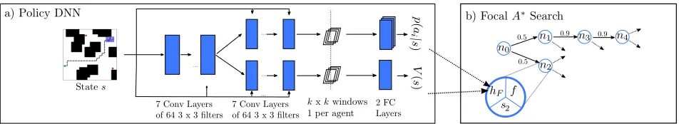
Figure 1:a)Policy network structure. It consists of one path for predicting action probabilitiesp(ai|s)for each robot, one for
predicting the plan length for all the robots.b)Focal A∗ωsearch. Example search path with action probabilities depicted on the
edges. The close-up shows information attached to each node: the statesi, thef-valuef(n)and the focal heuristichF(n).
Instead of specifying values of ω, Cohen et al. (2018) present ananytimeversion of A∗ωin which the search starts with high ω and tightens the bound iteratively. Whenever A∗ωreturns a solution pathP, the valueω¯ =c(P)/fminis a valid suboptimality bound, since the minimumf-value de-pends on an admissible heuristic and always under-estimates the cost of the optimal solution. (This is not true when us-ing classical A∗with non-admissible heuristics, since then the f-value itself depends on a non-admissible heuristic). Also, by design of A∗ω, it always holds thatω¯ ≤ω. Cohen et al. (2018) propose to continue search after a valid solution has been found, e.g. by choosingωnew= ¯ω−, where >0 is a small step size, which guarantees decreasing values of
ωsizes over time. Importantly, the anytime version can effi-ciently re-use the existing search tree when continuing with decreased values ofω.
3.2
Problem Description
We consider a fully-observable state spaceSon which a set ofNagents operate jointly. The agents perform joint actions
a = (a1, . . . , aN) ∈ Athat factor into one action ai for each agenti. Furthermore, we assume a known, determin-istic dynamics model of the environmentst+1 = f(st, at)
that maps a statest ∈ S and actionat ∈ Aat time stept
to the statest+1 at time stept+ 1. Functionc(s, a)∈ R+
defines a cost for each state-action pair. In addition, we have an initial configurationsinit, a set of invalid states{s}invalid which the system is not allowed to reach, as well as a set of goal states{s}goal. A control strategyπ : S → A is a mapping from state s ∈ S to action a ∈ A. The objec-tive is to construct a control strategy that drives the system from the initial state to any goal state while avoiding the invalid states. We refer to aproblem instance as the tuple
(S, A, f, c, sinit,{s}invalid,{s}goal). While we assume that the state spaceSand action setAremain invariant for all pos-sible problem instances, the initial, invalid, and goal states can change per instance.
Given a problem instance and a control strategy
π, the system path of length T is given by P = sinita0s1a1· · ·aT−1sT, whereat=π(st). A system path is
calledvalidif there existsT >0such thatsT ∈ {s}goaland
st ∈ {/ s}invalid,∀t = 0,· · ·, T. In addition, each valid path has an associated cost ofC(P) = PT−1
t=0 c(st, at). Then,
optimal planningis concerned with finding the control strat-egyπ∗that minimizes the cost of the resulting pathP∗.
3.3
Multi-Agent Policy via Imitation Learning
As mentioned earlier, we first train a DNN to imitate expert behaviors. The network takes an observation of the current state of a problem instance as input and generates distribu-tions over the set of acdistribu-tions A, i.e.,p(a|s)for each robot. Moreover, the same network also learns a value function
V(s)which estimates the minimum cost to reach the goal states for states∈S.
The structure of our proposed DNN, shown in Figure 1, is based on thesingle-agent policiespresented by Groshev et al. (2017) . The network consists of two predictive paths, one for the reactive policy and one for the value function. Each predictive path is composed of a series of 14 convo-lutional layers, consisting of 64 3×3 filters, followed by 2 fully connected layers. The first 7 convolutional layers are shared between the two paths. Moreover, each convolu-tional layer receives skip connections from the input. In the multi-agentcase, we extract a window of fixedk×k size aroundeachrobot’s position before entering the linear lay-ers, whereby the network becomes invariant to the number of agents. This may appear as only a small extension of Gro-shev et al. (2017), where only a single window is extracted. However, as we will show in our experiments, this makes a big difference in performance compared to learning policies for each agent individually. The final action probabilities are computed by a softmax activation function and all other ac-tivation functions are linear rectifiers.
We generate training data with an optimal planner, i.e., A∗, to solve sampled problem instances. Whenever the opti-mal planner could not solve an instance, we discard it from the training set. This yields training data that consists of op-timal state-action pairs as well as state-value-function pairs. For training, we use standardcross entropyas loss function for action probabilities and`1-norm for value predictions.
The whole setup might raise the question why learning to imitate an optimal planner and not directly use the optimal planner. One important reason is that in many applications the optimal planner can not produce a reasonable plan within given timing limits. Therefore, we propose to learn a guiding heuristicoff-linewhich helps to speed upon-lineplanning, as described in the next section.
3.4
Combine Learned Policy with Focal Search
net-work and act according to the learned policy, e.g., always act according to the most likely action. However, this ap-proach does not perform well due to the limited generaliza-tion ability of the network, as also shown in the quantitative numerical evaluation in Section 4. A more robust way is to use the learned policy to assist classical planners such as A∗. Groshev et al. (2017) propose to use the learned value func-tiondirectlyas planning heuristic. It considerably improves performance for some instances but invalidates optimality guarantees of the solution.
We solve this issue by combining the learned policy with focal A∗ω, introduced in Section 3.1. Specifically, we
pro-pose two novel approaches to design the focal heuristichF:
(i) Use the estimated value function from the learned net-work ashF. We refer to this algorithm as A∗ω,len. (ii) Use the path probability estimated by the learned policy ashF. This
algorithm is referred to as A∗ω,log. The motivation behind this focal heuristic is that it guides the search along paths that the learned action probabilities suggest.
The log-likelihood of a pathP = s0a0s1a1· · ·aT−1sT
is given bylogp(P) =PT−1
t=0 logp(at|st), wherep(at|st)
is the probability of choosing action at at statest. During
search, we would like to estimate the likelihood of the path through the node that is being evaluated. However, we only know the actions preceding the current time steptk>0. To
avoid bias towards the beginning of the path, we therefore assume a uniform policy for all succeeding steps up until a fixed horizon, i.e.,
logp(a0, .., atk, .., aT)≈
tk
X
i=0
logp(ai) + T
X
i=tk+1
log 1
|A|,
where we setTto the maximum number of steps of any node in the tree, and|A|is the cardinality of the set of actions.
Figure 1b depicts an example wheren2andn4 are cur-rently in the open list. UsinghFwith log-likelihood
estima-tion would prefern2overn4if we were only adding along the currently expanded path, sincelog(0.5)<log(0.5·0.9·
0.9). Normalizing to a common path length with the pro-posed method, however, prefers n4 because now the log-likelihood ofn2changes tolog(0.5·0.5·0.5).
Since we only modify the focal heuristichF in A∗ω, i.e.,
noth(n), we retain the guarantees on bounded suboptimal-ity. At the same time, the A∗ωsearch process is greatly accel-erated via using the learned heuristic as guidance.
4
Experimental Results
In the following, we present experimental results of apply-ing the proposed approach to the use case ofAutonomous Valet Parking(AVP). The resulting dynamic coverage prob-lem is computationally complex and cannot be solved opti-mally using A∗in acceptable time, which motivates the pro-posed use of learned heuristics with focal search.
4.1
Autonomous Valet Parking
An AVP system parks cars or picks up parked cars au-tonomously in public parking decks. Most existing solutions require extensive infrastructures such as a large number of
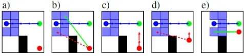
Figure 2: Execution of an optimal plan in a single-robot AVP example. a) The car (blue circle) has a fixed desired pathτc
(blue arrows) to reach its goal (green circle). b) Each cell of the car’s monitor region (shaded blue area) has to be ob-served by at least one robot. While the robot (red circle) can observe some cells (green solid arrow), the line-of-sight to other cells is occluded (dashed red arrow) by an obstacle (black area). c) The optimal strategy for the robot is to move two cells upwards, because the line-of-sight is still occluded in position (d). e) The monitor region is fully observable and the car can drive to the next cell along its path.
laser scanners, tracks, and shuttles to move cars. Such so-lutions are not only expensive, but also customized for spe-cific environment structures. These problems could be mit-igated by replacing static infrastructure with mobile robots that are equipped with sensors (mobile sensor units). Besides autonomously parking the car, a critical safety requirement is that the area in front of the car has to be monitored con-tinuously to ensure no collisions with obstacles or humans. Even though robot localization and navigation techniques are quite mature (Thrun, Burgard, and Fox 2005), the dy-namic coverage problem still has to be solved, i.e., where to position which mobile sensor unit for optimal execution time with minimal energy consumption. Instead of hand-crafted solutions, we propose to apply the proposed method to solve this dynamic coverage problem for multi-robot systems.
Modeling AVP: We model the AVP as a problem instance, described in Section 3.2, as follows. Assume a grid world with dimensionsDx, Dy ∈ N, where each cell cell(x, y),
with(x, y) ∈ W , {1, . . . , Dx} × {1, . . . , Dy}, is either
occupied by an obstacle or free. The desired path of the car
τc =sc1s
c
2· · ·s
c L, s
c
i ∈ W, is assumed to be provided by an
external planner. We haveR ∈ Nrobots available to guide the car along its path. The current state space is given by
S = (sr
1, sr2, . . . srR, sc), where sri ∈ W is the position of
robotiandsc ∈ τ
c is the position of the car. Note that the
car is assumed to only move along its path τc. The robots
can perform actions ar
i ∈ {up, down, lef t, right, none},
i.e., move to an adjacent cell within the grid world or stay still. Goal states are the terminal states of car paths, and in-valid states are the states where robots or the car collide into each other or into obstacles. Lastly, the car is only allowed to move to the next cell in its path when every cell in a monitor region is visible to at least one robot. This monitor region is defined as the set of cells surrounding the front of the car. As a cost functionc(a, s), we choose1for every time step until a goal state is reached, and in addition a cost of1 for every robot action. The robots are equipped with360◦
0 10 20 30 40 50 2
3 4 5
Number of epochs
Av
erage
loss
SPSW - training SPSW - validation
SPMW - training SPMW - validation
MPMW - training MPMW - validation
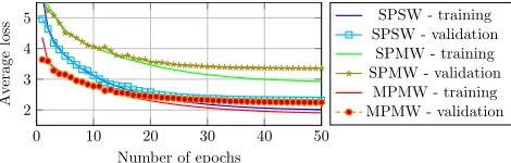
Figure 3: Learning curves during training, over training and validation set, as function of the number of training epochs.
whether a cell is visible for a robot or if the line-of-sight is occluded. Figure 2 depicts an example of a car path, the monitor region, the line-of-sight test, as well as execution of an optimal plan for the AVP problem.
4.2
Dataset Creation and Policy Learning
Training and Validation Dataset We generated a diverse set of problem instances (grid worlds of size20×20) for the AVP domain as described in Section 4.1 by randomly sam-pling numbers and shapes of obstacles, initial positions for the car and the robot(s), as well as the goal position for the car. In a first step, we computed the desired path for the car, ignoring the robots, using a python implementation of stan-dard A∗planner with Euclidean distance as heuristich. In a second step, an optimal planner based on A∗computed opti-mal action sequences for the robot(s) that minimize the ob-jective function. In this case the heuristichis the steps-to-go for the car. Since A∗is complete and the state space of the problem instances is finite, the optimal planner eventually returns for all instances, although in some complex cases only afterhoursof computing. Either it returns a valid so-lution or it fails when no soso-lution is possible, in which case we discard this instance. Finally, we added all intermediate states along the optimal path together with their respective optimal actions into the dataset.
Learning the Models For training, the network receives an observation of the current system state which contains the static map, the car path together with its current position along it, as well as the robots’ current positions. Specifically, a 3-layer tensor of dimensionW ×3from the current state of a grid world is created. The first layer contains a binary map of static obstacles, i.e.,cell(x, y)of this layer is1 if there is an obstacle, and0otherwise. The second layer consists of the car position and path, encoded ascell(xc
sc, yscc) = s c
/L,
sc ∈ {1, . . . , L}. Hence this also embeds the car goal po-sition. The third layer contains the robot positions, encoded as cell(xri, yir) = i,i ∈ {1, . . . , R}. The network outputs are then trained against the ground truth actions and value functions from the dataset, as described in Section 3.3.
4.3
Experiments and Results
We evaluated the ability of different policies to learn and, more importantly, generalize to new problem instances. Also, we examined the need to learntruemulti-robot poli-cies versus the possibility of applying single-robot polipoli-cies to multi-robot scenarios. For this, we used the following two
SPSW SPSW SPMW MPMW 1 rob. 2 rob. 2 rob. 2 rob.
mean acc. 0.84 0.045 0.25 0.64
std acc. 0.37 0.21 0.43 0.48
mean len. err. 0.88 17.67 1.26 0.81
std len. err. 3.83 8.40 4.53 3.00
Table 1: Performance of learned policies on the validation set. Comparison in terms of accuracy as the percentage of correctly predicted actions, and plan length prediction error. Mean and std values are computed on a per trial basis by forward simulating each world in the validation set.
experiments: (1) A comparison of the accuracy and perfor-mance between learning single vs multi-robot policies. (2) A comparison between the different strategies for solving the entire problem instances.
Learning single vs multi-robot models: In this experi-ment we learned three different DNN-models for single and multi-robot problem instances. To distinguish among the models, we denote them as follows:
• SPSW – Single-robot Policy over Single-robot Worlds: outputs action probabilities and a plan prediction for one single robot and is learned over problem instances with one single robot.
• SPMW – Single-robot Policy over Multi-robot Worlds: outputs action probabilities and plan prediction for one single robot but is learned over problem instances with two robots. In particular, the network selects only onek×
kwindow at the position of one of the robots, for which it outputs the action probability. This policy can also be seen as thedecentralizedcase, where each robot observes the full state but only controls its own actions.
• MPMW – Multi-robot Policy over Multi-robot Worlds: outputs action probabilities and plan prediction for two robots and is learned over problem instances with two robots. In contrast to SPMW, this reflects thecentralized case, where one policy controls all robots.
For this, we created two different test and validation datasets according to Section 4.2. The first contains problem in-stances where one single robot is in charge of escorting one car. The second contains instances with two robots escort-ing one car. To examine performance over trainescort-ing, we per-formed validation (with fixed weights) after each training epoch. All reported timing information in the experimental section refer to a server with2.10 GHzIntel(R) Xeon(R) E5-2695 v4 CPUs and a GTX 1080 TI graphics card.
Figure 4: Examples of solved problem instances. Each image depicts a full run to the goal state. a) Single-robot problem in-stance, solved perfectly just by applying the learned policy. b)-e) Multi-robot problem instances. b) Optimal solution computed by A∗ without time limit. A∗ could not find a solution in5 min. c) First solution computed by A∗∞,log after2.5 s, d) Refined solution by A∗ATafter five minutes. e) Directly applying the policy MPMW did not solve the problem.
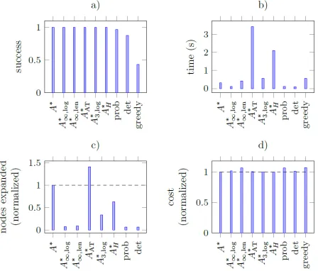
Figure 5: Comparing different policies solving 100 problem instances withonerobot using SPSW policies. a) Success rate. b) Computation time. c) Nodes expanded during search. d) Cost of the final solution, normalized to A∗.
networks were applied to multi-robot problem instances. Single-robot policies from SPSW and SPMW were applied to each robot, while MPMW already outputs control actions for all robots. For completeness also the values of SPSW applied to single robot dataset are shown in the table in the left column. The figure shows that merely applying single-robot policies, even if learned over multi-single-robot scenarios, leads to poor performance. Although learning single poli-cies over multi-robot scenarios (SPMW) leads to improved performances, it is still not sufficient to reach acceptable per-formance as indicated by the mean accuracy in Table 1. In other words, the results demonstrate that multi-robot coordi-nation must be learned jointly.
Application of learned heuristics: In this experiment we took the learned policies SPSW, SPMW and MPMW from
above and used them as learned heuristics in combina-tion with different control strategies. Each combinacombina-tion was tested on 100 randomly selected worlds from the respective validation sets. However, each problem instance was lim-ited to a maximal planning time of5 min(arbitrarily cho-sen). If this time was exceeded, the control strategies failed. Moreover, whenever the system reached an invalid state, the episode was terminated. In particular, we evaluated the fol-lowing control strategies:
• A∗: Classical planner without learned policy. Heuristic functionhis the steps-to-go for the car.
• Focal A∗, first solution(A∗∞,log): Focal search withω=
∞. This means that the search fully trusts the focal heuris-tic and returns after the first valid solution has been found. Its suboptimality bound can be computed after a solution is found (see Section 3.1). Using the learned policy to computehF with log-likelihood estimation.
• Focal A∗, first solution(A∗∞,len): As before, focal search withω =∞. Here the learned value function is used as focal heuristichF.
• Focal A∗(A∗3,log): Focal search withω = 3and learned log-likelihood estimation ashF.
• Anytime Focal A∗ (A∗AT): Focal search in anytime ver-sion, log-likelihood ashF.
• Groshev et al. (A∗H): Directly using the learned value function as heuristic in A∗ as proposed in Groshev et al. (2017)
• Greedy: Hand-crafted method to provide baseline bench-marks. The strategy employs available robots in the order of their relative distances to the monitored cells. Addi-tional robots are acquired if the already deployed ones are insufficient to cover the monitor region.
• Deterministic (det): The deterministic control strategy maps a state to the action with the highest probability.
Figure 6: Comparing policies for problem instances withtworobots. In all panels, blue and red bars correspond to using the SPMW or MPMW model, respectively. a) Success rates. b) Average planning time for all methods. c) Average cost of the returned environments, normalized to the optimal A∗, only problem instances for which A∗succeeded are considered.
until either a valid action is selected or until a maximum number of5trials is reached.
Figure 4 shows examples of a) one- and b)-e) two-robots problem instances from the validation set, solved using dif-ferent control strategies. Figure 4a depicts the solution of directly applying the learned policy (SPSW) as a probabilis-tic strategy in a one-robot instance. In this comparably easy example the policy solved the problem almost optimally, which shows that the DNN models have learned meaning-ful behavior.
This is in contrast to more complex scenarios with two robots, as depicted in Figure 4b-e. Panelbshows the ground truth solution, computed by A∗within18 min, and resulting in a cost of72. In the optimal solution, one of the robots es-corts the car close to its goal pose. At the end of its path the car ’parks’ close to a wall, which requires both robots to co-operate to observe the whole monitor region. Therefore, the second robot has to move to a location where it can monitor parts of the region that cannot be observed by the first robot. Here, directly applying the learned (MPMW) model did not lead to successful behavior (as shown in Figure 4e). Also, classical A∗ could not find a solution within5 min, while focal search guided by the learned heuristics found a first solution already after1 swith a resulting cost of 211. In this example, the cost of the returned path is three times the optimal solution, which by design is less than the plan-ner’s guarantee of ω = 6. Continuing focal search within the5 minplanning time refines the solution, as depicted in Figure 4d, resulting inω= 5andC(P) = 156.
The qualitative results illustrated in the example above also show up in quantitative analysis. Figure 5 shows the average results of 100 single-robot problem instances using SPSW strategies. The success rates of all A∗based methods are 1, while directly applying the learned probabilistic poli-cies result in a success rate around 0.96. However, A∗∞,log uses an order of magnitude less nodes to find a valid solution compared to A∗. The difference in computation time is not as big, since the network queries (of about5 msper query) increase computation time whenever the learned policy is used. Figure 5dshows the cost of the solutions, normalized over the solution of A∗. In the single robot case, all strategies found solutions that are close to the optimal.
The planning difficulty increases drastically when two robots are deployed due to the much larger state space. Fig-ure 6 shows results for SPMW (blue) and MPMW (red), av-eraged over 100 two-robot problems. In these complex sce-narios, A∗has a success rate of only0.9when planning time is limited to5 min. Also, directly applying the policies did not perform well and showed success rates of at most 0.6
when MPMW was applied using the probabilistic strategy. Directly using the learned heuristic in an optimal planner (A∗H), as proposed in Groshev et al. (2017), returns a suc-cess rate of about0.8. Our proposed method A∗∞,log using the learned MPMW heuristics as guidance returned a so-lution in all of the 100 validation scenarios. Moreover, our method found a first solution already within1 son average, with averageω= 7.2and a real suboptimality factor of3.1. Continuing the search for the remainder of the5 min plan-ning time window using A∗ATfurther reduced the value ofω
to4.2, with an actual suboptimality factor of2.0on average. Comparing the results for SPMW and MPMW in Figure 6 suggests that jointly learned multi-robot policies signifi-cantly outperform single-robot policies. Also note that, in general, focal A∗using log likelihood estimation as heuris-tic (A∗∞,log) surpasses value function estimation (A∗∞,len). In all plots, whenever we show normalized values, we only compare planning instances for which A∗ found a solution within the allowed planning time.
The results of our experiments show that directly apply-ing learned heuristics does not perform well in complex sce-narios. Using them as guiding heuristics improves perfor-mance considerably, though. Moreover, using (anytime) fo-cal search has the benefit of getting first solutions fast that can be refined over time, always having a guaranteed upper bound on the suboptimality factor.
5
Conclusion
still provide better performance, the proposed method re-quires much less manual engineering and, more importantly, is easily adaptable to different problem domains. Finally, we achieve guarantees for the qualities of our estimated solu-tions with respect to optimal solusolu-tions by combining an ex-isting focal search algorithm with our learned heuristics.
Since the network already produces a policy and a value function, further work in reinforcement learning seems to be an obvious path to follow in future work. Specifically, we are interested in learning policies in even more complex tasks, such as problem instances with more than two agents for which optimal ground truth is not available.
References
Arfaee, S. J.; Zilles, S.; and Holte, R. C. 2011. Learn-ing heuristic functions for large state spaces. Artif. Intell. 175(16-17):2075–2098.
Arya, V.; Garg, N.; Khandekar, R.; Meyerson, A.; Muna-gala, K.; and Pandit, V. 2004. Local search heuristics for k-median and facility location problems. SIAM Journal on computing33(3):544–562.
Burgard, W.; Moors, M.; Stachniss, C.; and Schneider, F. E. 2005. Coordinated multi-robot exploration. IEEE Transac-tions on robotics21(3):376–386.
Cohen, L.; Greco, M.; Ma, H.; Hernandez, C.; Felner, A.; Kumar, T. K. S.; and Koenig, S. 2018. Anytime focal search with applications. In Proceedings of the Twenty-Seventh International Joint Conference on Artificial Intel-ligence, IJCAI-18, 1434–1441. International Joint Confer-ences on Artificial Intelligence Organization.
Cortes, J.; Martinez, S.; Karatas, T.; and Bullo, F. 2002. Coverage control for mobile sensing networks. InRobotics and Automation, 2002. Proceedings. ICRA’02. IEEE Inter-national Conference on, volume 2, 1327–1332. IEEE. Cybenko, G. 1989. Approximation by superpositions of a sigmoidal function. Mathematics of control, signals and systems2(4):303–314.
Dijkstra, E. W. 1959. A note on two problems in connexion with graphs.Numer. Math.1(1):269–271.
Ernandes, M., and Gori, M. 2004. Likely-admissible and sub-symbolic heuristics. InProceedings of the 16th Euro-pean Conference on Artificial Intelligence, 613–617. Cite-seer.
Ghallab, M.; Nau, D.; and Traverso, P. 2004. Automated Planning: theory and practice. Elsevier.
Groshev, E.; Tamar, A.; Srivastava, S.; and Abbeel, P. 2017. Learning generalized reactive policies using deep neural net-works.CoRRabs/1708.07280.
Hart, P. E.; Nilsson, N. J.; and Raphael, B. 1968. A for-mal basis for the heuristic determination of minimum cost paths.IEEE transactions on Systems Science and Cybernet-ics4(2):100–107.
Helmert, M., and Domshlak, C. 2009. Landmarks, critical paths and abstractions: what’s the difference anyway? In ICAPS, 162–169.
Krizhevsky, A.; Sutskever, I.; and Hinton, G. E. 2012. Imagenet classification with deep convolutional neural net-works. InAdvances in neural information processing sys-tems, 1097–1105.
Latombe, J.-C. 2012. Robot motion planning, volume 124. Springer Science & Business Media.
LaValle, S. M. 2006. Planning algorithms. Cambridge university press.
Lee, S. G.; Diaz-Mercado, Y.; and Egerstedt, M. 2015. Mul-tirobot control using time-varying density functions. IEEE Transactions on Robotics31(2):489–493.
Mnih, V.; Kavukcuoglu, K.; Silver, D.; Rusu, A. A.; Ve-ness, J.; Bellemare, M. G.; Graves, A.; Riedmiller, M.; Fidjeland, A. K.; Ostrovski, G.; et al. 2015. Human-level control through deep reinforcement learning. Nature 518(7540):529.
M¨ulling, K.; Kober, J.; Kroemer, O.; and Peters, J. 2013. Learning to select and generalize striking movements in robot table tennis. The International Journal of Robotics Research32(3):263–279.
Pearl, J., and Kim, J. H. 1982. Studies in semi-admissible heuristics. IEEE Transactions on Pattern Analysis and Ma-chine IntelligencePAMI-4(4):392–399.
Russell, S. J., and Norvig, P. 2016. Artificial intelligence: a modern approach. Malaysia; Pearson Education Limited,. Samadi, M.; Felner, A.; and Schaeffer, J. 2008. Learning from multiple heuristics. InAAAI, 357–362.
Sartoretti, G.; Wu, Y.; Paivine, W.; Kumar, S.; Koenig, S.; and Choset, H. 2018. Distributed reinforcement learning for multi-robot decentralized collective construction. In Pro-ceedings of the International Symposium on Distributed Au-tonomous Robotics Systems (DARS), (in print).
Sutskever, I.; Vinyals, O.; and Le, Q. V. 2014. Sequence to sequence learning with neural networks. InAdvances in neural information processing systems, 3104–3112. Tamar, A.; Wu, Y.; Thomas, G.; Levine, S.; and Abbeel, P. 2016. Value iteration networks. InAdvances in Neural In-formation Processing Systems, 2154–2162.