The Thirty-Third AAAI Conference on Artificial Intelligence (AAAI-19)
Less but Better: Generalization Enhancement
of Ordinal Embedding via Distributional Margin
Ke Ma,
1,2Qianqian Xu,
3Zhiyong Yang,
1,2Xiaochun Cao
1,2∗1State Key Laboratory of Information Security, Institute of Information Engineering, Chinese Academy of Sciences 2School of Cyber Security, University of Chinese Academy of Sciences
3Key Laboratory of Intelligent Information Processing, Institute of Computing Technology, Chinese Academy of Sciences
{make, yangzhiyong, caoxiaochun}@iie.ac.cn, [email protected]
Abstract
In the absence of prior knowledge, ordinal embedding meth-ods obtain new representation for items in a low-dimensional Euclidean space via a set of quadruple-wise comparisons. These ordinal comparisons often come from human annota-tors, and sufficient comparisons induce the success of clas-sical approaches. However, collecting a large number of la-beled data is known as a hard task, and most of the ex-isting work pay little attention to the generalization abil-ity with insufficient samples. Meanwhile, recent progress in large margin theory discloses that rather than just maximiz-ing the minimum margin, both the margin mean and variance, which characterize the margin distribution, are more crucial to the overall generalization performance. To address the is-sue of insufficient training samples, we propose a margin dis-tribution learning paradigm for ordinal embedding, entitled Distributional Margin based Ordinal Embedding (DMOE). Precisely, we first define the margin for ordinal embedding problem. Secondly, we formulate a concise objective func-tion which avoids maximizing margin mean and minimiz-ing margin variance directly but exhibits the similar effect. Moreover, an Augmented Lagrange Multiplier based algo-rithm is customized to seek the optimal solution ofDMOE effectively. Experimental studies on both simulated and real-world datasets are provided to show the effectiveness of the proposed algorithm.
The problem of analyzing a set of n objects given simi-larity information is an inherent part in a broad variety of tasks in artificial intelligence (Heikinheimo and Ukkonen 2013; Wilber, Kwak, and Belongie 2014), machine learn-ing (Jamieson and Nowak 2011; Kleindessner and Luxburg 2014; Arias-Castro 2017; Kleindessner and von Luxburg 2017), information retrieval (Liu et al. 2016), data mining (Le and Lauw 2016) and computer vision (Wilber et al. 2015). Many algorithms are based on the assumption that ‘similar’ inputs should generate ‘close’ outputs. In a numer-ical setting of embedding, a similarity function (or, equiva-lently, a dissimilarity function) quantifies how ‘similar’ ob-jects are to others. The required input is the distance or simi-larity matrix of items. We calculate a set of embedded points which aims to preserve such similarities as well as possible. However, in recent years a whole new branch of the
liter-∗
The corresponding authors.
Copyright c2019, Association for the Advancement of Artificial Intelligence (www.aaai.org). All rights reserved.
ature has emerged, which is the comparison-based embed-ding. Instead of evaluating similarity directly, we collect the similarity comparisons as follows:
“Is the similarity between objectiand jlarger than the similarity betweenlandk?”
The corresponding problem is ordinal embedding. These two types of supervision information, numerical similari-ties and relative comparisons, are all generated by human beings. Nevertheless, the latter one provides similarity esti-mates on a relative scale instead of the absolute scale. The comparison-based setting is a special case of the observation that humans are better at comparing two stimuli than at iden-tifying a single one (Stewart, Brown, and Chater 2005). Con-sequently, the relative comparison is a more reliable form for incorporating human knowledge with artificial intelligence tasks.
The ordinal embedding problem was firstly studied by (Shepard 1962a; 1962b; Kruskal 1964a; 1964b) in the psy-chometric society. In recent years, it has drawn a lot of at-tention (Schultz and Joachims 2003; Agarwal et al. 2007; Tamuz et al. 2011; van der Maaten and Weinberger 2012; Terada and Luxburg 2014; Amid and Ukkonen 2015; Heim et al. 2015; Jain, Jamieson, and Nowak 2016; Ma et al. 2018). One class of these typical methods is margin-based ordinal embedding which solves the problem under the clas-sification framework. The well-known Generalized Non-Metric Multidimensional Scaling (GNMDS) (Agarwal et al. 2007) aims at finding a Gram matrixGsuch that the pair-wise distances of embedded points satisfy the partial or-der constraints. Stochastic Triplet Embedding (STE/TSTE) (van der Maaten and Weinberger 2012) is proposed to jointly penalize the violated constraints and reward the satisfied constraints via logistic loss. Multi-view Triplet Embedding (MTE) (Amid and Ukkonen 2015) decomposes the STE
comparison-based scenarios. With this limitation, SPE and LOE are not suitable for ordinal embedding via quadruplets or triple comparisons.
A common issue of the existed ordinal embedding meth-ods is the dependence of large samples of similarity com-parisons. (Kleindessner and Luxburg 2014; Arias-Castro 2017) show the consistency of ordinal embedding prob-lem. When the number of the objects n tends to infin-ity, the set of embedded points always converges to the set of original points, up to similarity transformations; the rate of convergence depends on the Hausdorff distance be-tween the ground-truth points. Later (Jain, Jamieson, and Nowak 2016) show a finite sampling result of consistency. Learning an embedding which predicts nearly as well as the true embedding needsΘ(pnlogn)samples, wherepis the embedding dimension. There is a strong condition that the triple-wise comparisons are generated from the classical Bradley-Terry-Luce (BTL) model (Bradley and Terry 1952; Luce 1959) and this assumption could not be verified in the actual applications. The theoretical results suggest that only the adequateness of similarity comparisons can promise the prediction result. However, the cost of eliciting relative simi-larity comparisons from human beings would be prohibitive. The amenable applications for collecting the relative simi-larity comparisons, e.g., crowdsourcing and human compu-tation, need passively waiting for participants and stimulate them with money to get the desired information. Without prior knowledge, the relative comparisons always involve all objects, and the number of possible comparisons could be Θ(n4). The spending of data collection presents ordinal
em-bedding methods with a dilemma: the insufficient samples would limit the potential performance; the adequate sam-ples with prospective results would be cumbersome. Unfor-tunately, most of the traditional methods ignore that the gen-eralization is the main concern in ordinal embedding task with insufficient samples.
In this paper, we propose a new method, named Distri-butional Margin based Ordinal Embedding (DMOE), which tries to achieve strong generalization performance by opti-mizing the margin distribution in ordinal embedding prob-lem. Inspired by the recent results in classification (Zhang and Zhou 2014; Yang, Lu, and Zhang 2016), we define the margin of ordinal embedding and characterize the margin distribution by the first- and second-order statistics, and try to maximize the margin mean and minimize the margin vari-ance simultaneously. For optimization, we propose an alter-nating direction method of multipliers (ADMM) forDMOE
with semi-definite and low-rank constraints. Comprehensive experiments on the synthetic and real-world datasets show the superiority of our method to other ordinal embedding al-gorithms, verifying that the margin distribution is more cru-cial for generalization than minimum margin.
Problem Definition
Throughout the paper, scalars, vectors, matrices and sets are denoted as lowercase letters (x), bold lower case letters (x), bold capital letters (X) and calligraphy uppercase let-ters (X).xij denotes the(i, j)entry ofX.[n]is the set of
{1, . . . , n}.E(·)represents the expectation.
Suppose O = {o1, . . . ,on} is a set of n objects, we
assume that a certain but unknown similarity function ζ : O × O → R+ assigns similarity value ζij for a pair of
objects (oi,oj). With similarity function ζ, a quadruplet
q = (i, j, l, k)defines the corresponding ordinal constraint, and these constraints lead to the ordinal embedding problem. Definition 1(Ordinal Constraints). Given a set of quadru-plets
Q={q | q= (i, j, l, k),(i, j)6= (l, k),
i6=j, l6=k, i, j, l, j∈[n]} (1)
which is a subset of [n]4, the ordinal constraints Y
Q =
{yq|q ∈ Q} ⊂ {−1,+1}|Q|, implies the similarity partial
order of object pairs inOas
yq =
+1, if ζij < ζlk,
−1, if ζij > ζlk. (2)
Our goal here is to obtain a set of embedded points X which satisfy the ordinal constraints Q. Without prior knowledge, embeddingOinto a Euclidean spaceRpis the most common situation which assumes that the squared Eu-clidean distances among embedded points are inversely pro-portional to the unknown similarity values. Specifically, a large distance of two embedded pointsd2
ij = kxi −xjk22
means the corresponding objectsoiandojwould have small
similarity value ζij. This assumption connects the squared
Euclidean distances ofXand ordinal constraintsQ. We fur-ther give the formal definition of ordinal embedding.
Definition 2(Ordinal Embedding). SupposeQis a collec-tion of quadruplets which are drawn independently and uni-formly at random and YQ is the correspondence ordinal
constraints of object setO. LetX ={x1, . . . ,xn} ∈Rp×n
is the desired embedding in the Euclidean spaceRp where
p nandD = {d2ij} ∈ Rn×n is the squared Euclidean
distance matrix of embeddingX. Ordinal embedding is the problem of obtainingX with ordinal constraintsYQonD
such that
sign(yq·∆qD)>0, ∀yq ∈ YQ,
where
∆qD=d2ij−d
2
lk=kxi−xjk22− kxl−xkk22.
Note that one cannot consistently estimate the underly-ing embeddunderly-ing X with only ordinal supervision and with-out direct observations. In the case when no direct measure-ments are available, say the metric information ofOas the input, the underlying embeddingXis only identifiable up to certain monotonic transformations,e.g., rotation, reflection, translation, and scaling. Therefore, the sign consistency is adopted as the goal of ordinal embedding.
By the above definition, the margin of instance(Xq, yq)
can be naturally defined as
γq=yq·∆qD, (3)
whereXq ={xi,xj,xl,xk}, ∀q∈ Q.
Despite the close relationship betweenDandX,∆qD
matrix ofXand construct a margin function as a linear func-tion of Gram matrix. Firstly, a map is established to connect the distance matrixDand the Gram matrixG=X>X:
dij = gii−2gij+gjj
D = diag(G)·1>−2G+1·diag(G)>,
wherediag(G)is the column vector composed of the diag-onal entries ofGand1is then-dimension vector with all entries being1. With a little abuse of∆q, the margin of
in-stance(Xq, yq)can be written as
γq = yq·∆qD=yq(dij−dlk)
= yq(gii−2gij+gjj−gll+ 2glk−gkk)
:= yq·∆qG, ∀q∈ Q.
(4)
By the definition of (4), ordinal embedding can be formu-lated as the following convex optimization problem.
Definition 3(The Margin-based Ordinal Embedding). Let
l:R+→
Rbe a loss function which satisfies
l(x) :
> 0, ifx >0,
≤ 0, ifx <0. (5)
Given the ordinal constraints YQ, the ordinal embedding
problem can be formulated as a semi-definite programming of Gram matrixG:
min
G L(G,YQ)
s.t. G0, rank(G)≤p, (6)
whereL(G,YQ) = |Q|1 P q∈Q
l(γq).
We note that (6) is a semi-definite programming (SDP) and G 0 comes from the fact that G = X>X is a positive semi-definite matrix. Furthermore, the desired em-bedding dimension pis a parameter of the ordinal embed-ding. It is well known that there exists a perfect embedding X estimated by any label setY on the Euclidean distances inRn−2, even for the noisy constraints (Borg and Groenen 2003). However, the low-dimensional setting wherepn
is the main task of this work. The smallestpfor noisy ordinal constraintsYQis a future direction which worths pursuing.
The choice ofpin the experiment section depends on the potential applications.
For example, the Generalized Non-metric Multidimen-sional Scaling (GNMDS) follows the SVM formulation to obtain theGby solving
min G,ξ
1 |Q|
X
q∈Q
ξq
s.t. γq ≥γ0−ξq, ξq ≥0, ∀q∈ Q,
G0, rank(G)≤p,
(7)
whereγ0is a relaxed minimum margin andξ={ξq}q∈Qis
the slack variable.
Distributional Margin based Embedding
The relaxed minimum margin γ0 in GNMDS indeedcharacterizes the top minimum margins of all instance {Xq, yq}q∈Q. In margin theory of classification, it is known
that maximizing the minimum margin of training examples is not sufficient to achieve fulfilling generalization perfor-mance (Reyzin and Schapire 2006). The margin distribution of training examples, rather than the minimum margin, is more crucial to generalization performance in classification (Gao and Zhou 2013; Zhang and Zhou 2016).
Formulation
The two most usual statistics for characterizing the margin distribution are the first- and second-order statistics, that is, the mean and the variance of margin. According to (4), the margin mean of training samples{(Xq, yq)}is
¯
γ = 1 |Q|
X
q∈Q
γq (8)
and the margin variance is
ˆ
γ= 1 |Q|
X
q∈Q
(γq−γ¯)2. (9)
Intuitively, we attempt to maximize the margin mean and minimize the margin variance simultaneously in ordinal em-bedding problem (6).
First, there is a straightforward idea to achieve our goal as considering the margin mean (8) and the margin variance (9) in (6) explicitly. Although (6) can adopt different loss functions, we will focus on SVM formulation (7) because the hinge loss is a natural form of margin. Considering the margin distribution, the optimization problem (7) can be for-mulated as
min G,ξ
1 |Q|
X
q∈Q
ξq−λ1γ¯+λ2γˆ
s.t. γq ≥γ0−ξq, ξq ≥0, ∀q∈ Q,
G0, rank(G)≤p,
(10)
whereλ1andλ2are the trade-off parameters for balancing
the impacts ofγ¯andγˆ. It is apparent thatGNMDS(7) is a degenerate case of (10) when λ1andλ2 equal to0.
How-ever, there exists an obvious drawback of (10) with directly optimizing the margin distribution: tuning the parameters,
λ1andλ2, is an obstacles of solving (10) efficiently.
There-fore, a new lightweight formulation is proposed to optimize margin distribution implicitly.
Recall thatSVMfixes the minimum margin as1by scal-ing the margin with the norm of linear predictor. Followscal-ing the similar way, we can scale the margin of(Xq, yq)in
or-dinal embedding (4) and set the margin mean as a constant. This would not result in a sub-optimal solution because the ordinal constraintsYQcan only determine an embeddingX
up to the monotonic transformations. Without loss of gener-ality, the mean ofγQ={γq|q∈ Q}can be set as a constant
and an equality constraint is conducted 1
|Q|
X
q∈Q
On the other hand, we want to minimize the variance ofγQ. By (11), the deviation ofγq to the margin meanγ˜0is|γq−
˜
γ0|, and we force the deviation to be smaller thanεq ≥0as
|γq−γ˜0| ≤εq, ∀q∈ Q. (12)
Thus, minimizingεq is equivalent to minimize the margin
variance (9). Meanwhile, (12) implies the margin mean con-straint (11).
Constraints like (12) in optimization problems always in-volve two inequality,∀q∈ Q,
γq ≤˜γ0+εq, (13a)
γq ≥˜γ0−εq. (13b)
Note that the soft-margin constraint
γq≥γ˜0−ξq (14)
plays the same role as (13b). Replacing (13b) with (14) and adding (13) into (10), we arrive at the following formulation
min G,ξ,ε
1 |Q|
X
q∈Q
ξq+ν·εq
s.t. γq ≥˜γ0−ξq, γq≤γ˜0+εq,
ξq ≥0, εq ≥0, ∀q∈ Q,
G0, rank(G)≤p.
(15)
This optimization problem corresponds to dealing with such a loss function,∀q∈ Q
`γ˜0,ν(γq) = max(˜γ0−γq,0) +ν·max(γq−˜γ0,0).
(16) The trading-off parameterν in (15) can capture the asym-metry between the sign correctness and the dispersion of {γq}q∈Q. Whenν = 1and ignoring the semi-definite and
rank constraints, (15) is similar to the support vector regres-sion (SVR) (Drucker et al. 1997). InSVR, theτ-insensitive loss
|ζ|τ =
0, if|ζ| ≤τ,
|ζ| −τ, otherwise (17) produces two slack variablesξandξ∗for each training
ex-ample to guard against outliers. Asν = 1, the loss function (16) is explicitly the same loss function adopted bySVRas
τ= 0. In our formulation (15),ξqandεqconduct the similar
constraints likeSVRbut have totally different meanings. All the training examples are used to learn the margin distribu-tion in (15), but the optimal soludistribu-tion ofSVRis only spanned by the support vectors which is sparse in the training data. Figure 1 depicts the situations of the learned margin distri-bution graphically. Some theoretical results are provided at the end of this section.
Theorem 1. Suppose that
Gµ={G∈Sn+: kGk∞≤µ,kGk∗≤λ}
and the true Gram matrixG∗ ∈ Gµ. LetGˆ be a solution of
(15). With probability at least1−δ, it holds that
R( ˆG)−R(G∗)
≤ 4µ(1 +ν)
s
32nplogn
|Q| + 8µ(1 +ν)
s
2 log2δ |Q| ,
(18)
(a) Margin Distribution (b) Loss Function
Figure 1: (a) The Margin Distribution obtained by solving (15). (b) The loss function (16) with differentν.
whereR(·)is the risk, as for anyG∈ Gµ
R(G) =E[`(γq)] =
1 |Q|
X
q∈Q
pq`(γq) + (1−pq)`(−γq),
pq =P(yq = 1). Here the expectation respects to both the
uniformly random selection of the quadrupletqand its label
yq.
Theorem 1 says that |Q| must scale like Θ(pnlogn) which leads to the bounded errorR( ˆG)−R(G∗). This result is consistent with known finite sample bounds (Jamieson and Nowak 2011). The details are provided in the supplementary materials. The generalization bound of margin distribution is a future direction.
Optimization
Consider that∆qis a linear operator onSn+,∆qhas its
sym-metricn×nmatrix form inSn+, the positive semi-definite
cone ofn×nsymmetric matrix. Given a ordinal constraints
q= (i, j, l, k),Kq is the matrix form of∆qwhere
Kq =
i j l k
i 1 −1 0 0
j −1 1 0 0
l 0 0 −1 1
k 0 0 1 −1
(19)
and
∆qG=hKq,Gi=tr(KqG) =vec(Kq)>vec(G). (20)
With the trick that
˜
γ0−γq =yqyqγ˜0−yq∆qG=yq(yqγ˜0−∆qG), (21)
we note
eQ = [e1, . . . , e|Q|]>
= yQΓ0−
.. .
vec(Kq) >
.. .
|Q|×n2
·vec(G)
, yQΓ0− K ·vec(G),
(22)
where yQ ∈ {−1,+1}|Q| = [y
1, . . . , y|Q|]>, Γ0 is a
|Q|-dimension vector with all entries areγ˜0 and is the
solved by the ALM framework efficiently. The optimization is converted into:
min
T k(yQe1)+k p
p+k(yQe2)+kpp+λkG1k∗
s.t. G=G1, G=G2, G20,
e1=eQ, e2=−eQ,
(23) whereT ={G,G1,G2,e1,e2}is the set of all the
param-eters to be solved andk · k∗ is the nuclear norm which is
the convex surrogate of matrix rank constraints. It is worth mentioning that (23) is a convex optimization problem as the feasible set of each constraint is a convex set and the objec-tive function is convex. The Lagrange function of (23) can be written in the following form:
L(T) = k(yQe1)+k+k(yQe2)+k
+ Φ(z1,e1−eQ) + Φ(z2,e2+eQ)
+ λkG1k∗ + Φ(Z3,G−G1)
+ δ(G20) + Φ(Z4,G−G2),
(24)
with
Φ(u,v) = µ 2kvk
2+hu,vi, µ >0.
k · kis`2norm for vector and the Frobenius norm for
ma-trix. In addition, z1,z2 ∈ R|Q| andZ3,Z4 ∈ Rn×n are Lagrange multipliers. δ is the Dirac delta function whose function value would be infinity if the condition is not satis-fied. Below are the solutions to each sub-problem.
e1 sub-problem.With the variables unrelated toe1 fixed,
we have the sub-problem ofe1:
e(1t+1)= arg min e1
1
µ(t)k(yQe1)+k
p p+
1
2ke1−s
(t) 1 k
2 2,
(25) where
s(1t)=e(Qt)−z
(t) 1
µ(t).
It’s worth noting that(·)+ is a piece-wise linear function.
Thus, to seek the minimum of each element ine1, we just
need to pick the smaller value betweenyqe1q and0. The
so-lution of (25) is
e(1t+1)= Ω
S 1 µ(t)
[s(1t)]
+ ¯Ωs(1t), (26)
whereΩ :RQ→RQis an indicator function as[Ω(w)] q =
I(wq > 0)·wq, w ∈ RQ andΩ¯ is the complementary support ofΩ. The definition of shrinkage operator on scalars isSτ >0[u] = sign(u)(|u| −τ)+and it is an element-wise
operator for vector and matrix.
e2sub-problem.Similarly, picking out the terms related to
e2gives the following sub-problem:
e(2t+1)= arg min e2
1
µ(t)k(yQe2)+k
p p+
1
2ke2−s
(t) 2 k
2 2,
(27) where
s(2t)=−e(Qt)−z
(t) 2
µ(t),
and the solution ofe2 sub-problem is just replaced thes (t) 2
withs(1t)in (26).
G sub-problem. Dropping the terms independent on G leads to the following problem:
arg min G
Φ(z(t)
1 ,e (t)
1 −e
(t)
Q) + Φ(z
(t) 2 ,e
(t)
2 +e
(t)
Q)
+ Φ(Z(3t),G−G(1t)) + Φ(Z(4t),G−G(2t))
.
(28) We have
2(K>K+I)·vec(G)(t+1)
= K>
e(1t)+ 1
µ(t)z (t)
1 −e
(t)
2 −
1
µ(t)z (t) 2
+ vec
G(1t)− 1
µ(t)Z (t)
3 +G
(t)
2 −
1
µ(t)Z (t) 4
,
(29)
and note the right-hand side asw, we have
vec(G)(t+1)=1 2(K
>K+I)−1w,
andG(t+1)is the matrix form ofvec(G)(t+1).
G1 sub-problem. There are two terms in (24) involving
G1. The associated optimization problem ofG1is
G(1t+1)= arg min G
λkG1k∗+ Φ(Z3,G−G1), (30)
and solving this problem yields
G(1t+1)=US λ µ(t)
(Σ)V>, (31)
where
G(1t)+ 1
µ(t)Z (t)
3 =UΣV
>
andSτ(·)is the shrinkage operator.
G2sub-problem. Considering the potential asymmetric of
G(t), we claim that G2 is the nearest symmetric positive
semi-definite matrix of G(t) in Frobenius norm (Higham 1988). By the following theorem, we show the explicit solu-tion ofG(2t).
Theorem 2. Suppose thatA∈Rn×n, and letB = (A+ A>)/2, C = (A−A>)/2 be the symmetric and skew-symmetric parts of Arespectively. If we do polar decom-position of B as B = U H where U is orthogonal ma-trix U U> = I and H is positive semi-definite matrix,
XF = (B+H)/2is the unique approximation ofAin the
Frobenius norm with positive semi-definite constraint, and the distanceρF(A)in the Frobenius norm fromAtoSn+is
ρ2F(A) = X
σi(B)<0
σi2(B) +kCk2F,
whereσi(B), i= 1, . . . , nis the eigenvalue ofB.
Consequently, the explicit solution ofG(2t)is
G(2t) = 1 4
G(t)+
1
µZ4+G
>
(t)+
1 µZ > 4 + 1 4 s
G(t)+
1
µZ4
> G(t)+
1
µZ4
,
where√Ais the square root ofA ∈ Sn+,A = V SV− 1
and√A = V S12V−1,S is a diagonal matrix and S 1 2 is
element-wise square root ofS.
Algorithm 1:The ADMM method for solving(23) Input:K,yQ,γ0,ν,λ
Output:G
1 InitializeG0,µ,z (0)
1 =z
(0)
2 =0|Q|,t:= 1,
Z(0)1 =Z(0)2 =0n×n, calculateeQvia (22);
2 whileNot Convergeddo
3 updatee1,e2by solving (25) and (27);
4 updateGby solving (28); 5 updateG1,G2via (31) and (32);
6 calculateeQvia (22);
7 update multipliers andµas
z(1t+1) = z(1t)+µ(t)(e(1t)−eQ)
z(2t+1) = z(2t)+µ(t)(e(2t)+eQ)
Z(1t+1) = Z(1t)+µ(t)(G(t)−G(1t))
Z(2t+1) = Z(2t)+µ(t)(G(t)−G(2t))
µ(t+1) = ρµ(t), ρ >1
(33)
t:=t+ 1; 8 end
For clarity, the procedure of solving (23) is outlined in Algorithm 1. The algorithm would not be terminated until the change of objective value in two successive iterations is smaller than a threshold (in the experiments, 0.001 is the default setting).
Empirical Study
In this section, we show the results of simulations and real-world data experiments to demonstrate the effectiveness of the proposed algorithms. As the existed margin-based ordi-nal embedding methods, such as GNMDS, STE and TSTE, just use triple-wise comparisons as the ordinal constraints, we treat triple-wise comparisons as the input of the proposed algorithm for fair competition. The triple-wise comparisons T ={(i, j, k)}is a special case of quadruplets which means
l=iinq= (i, j, l, k)∈ Q. The∆pof triplett= (i, j, k)is
also a symmetricn×nmatrix indicated by(i, j, k)as
Kt=
i j k
!
i 0 −1 1
j −1 1 0
k 1 0 −1
. (34)
Replacing Kq with Kt in those sub-problems in
Al-gorithm 1, the proposed DMOE method could handle the triplets set T as the ordinal constraints. The reproducible code can be found here1.
1
https://github.com/alphaprime/DMOE
Simulation
Settings. The synthesized dataset consists of 100 points {xi}100i=1 ⊂ R10, where xi ∼ N(0,201I), I ∈
R10×10 is the identity matrix. The possible similarity triple comparisons are generated based on the Euclidean distances between {xi}. We randomly sample |T | =
{200,500,1,000,10,000}triplets as the training set and the test set is the rest of all triplets. The embedding dimension is fixed to10.
Evaluation Metrics.We employ the generalization error to evaluate generalization ability of various algorithms. As the learned Gram matrixGfrom partial triple comparisons set T ⊂ [n]3 may be generalized to unknown triplets, the per-centage of held-out triplets which is not satisfied in theGis the generalization error of the learned embedding.
Competitors. We compare the proposed algorithm with three well-known ordinal embedding methods: GNMDS (Agarwal et al. 2007), STE and TSTE (van der Maaten and Weinberger 2012). Note that we adopt the optimization strat-egy proposed by (Jain, Jamieson, and Nowak 2016), which performs gradient descent with line search, and projects the Gram matrix onto the subspace spanned by the topp eigen-values at each step (i.e. setting the smallestn−peigenvalues to0). We call the three competitors: GNMDS-p, STE-pand TSTE-p, correspondingly. The optimization problem of GN-MDS is (7). STE replaces the hinge loss by logistic loss in (7) and adopts Gaussian kernel to predict the label:
lste(G(t), yp) = log(1 + exp(γp(t))),
where γp(t) = ∆pG(t). TSTE employs the heavy-tailed
Student-t kernel:
ltste(G(t), yp) = log
1 +γp(t)−
α+1
2
.
The regularization parameters of the competitors are tuned for the best performance under the different settings.
(a)200 (b)1000 (c)10000
Figure 2: Generalization errors of DMOE, GNMDS-p,
STE-pand TSTE-pon the synthetic dataset.
Table 1: Performance Comparison on synthetic dataset with200,1000and10000samples as training data, respectively
(a)200samples
algorithm min median max std
GNMDS-p 0.419 0.447 0.476 0.016 STE-p 0.397 0.426 0.461 0.016 TSTE-p 0.440 0.468 0.498 0.014 DMOE 0.372 0.390 0.410 0.011
(b)1000samples
min median max std
0.318 0.341 0.359 0.009 0.375 0.385 0.401 0.007 0.426 0.441 0.466 0.011 0.281 0.298 0.305 0.008
(c)10000samples
min median max std
0.143 0.147 0.154 0.007 0.219 0.234 0.251 0.007 0.238 0.257 0.271 0.011 0.142 0.146 0.151 0.008
Table 2: Performance Comparison on music artists dataset with200,500,1000and5000samples as training data.
(a)200samples
algorithm min median max std
GNMDS-p 0.391 0.403 0.416 0.007 STE-p 0.444 0.455 0.475 0.008 TSTE-p 0.416 0.436 0.458 0.011 DOME 0.372 0.385 0.400 0.007
(b)1000samples
min median max std
0.307 0.317 0.332 0.007 0.397 0.415 0.429 0.007 0.377 0.389 0.406 0.007 0.281 0.291 0.307 0.007
(c)5000samples
min median max std
0.225 0.239 0.257 0.006 0.252 0.275 0.294 0.011 0.243 0.259 0.297 0.013 0.216 0.227 0.244 0.007
the margin distribution instead of maximizing the mini-mum margin like the classic methods. Third, the results of GNMDS-pverifies that only maximizing the minimum mar-gin would not necessarily lead to better generalization per-formances as the STE-pis better than GNMDS when train samples are few.
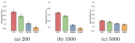
(a)200 (b)1000 (c)5000
Figure 3: Generalization errors of DMOE, GNMDS, STE and TSTE on the music artists dataset.
Music Artist Data
Settings. The music artist data is collected by (Ellis et al. 2002) via a web-based survey in which 1,032 users pro-vided213,472triplets on the similarity of412music artists. We use the data pre-processed by (van der Maaten and Wein-berger 2012) which includes only9,107triplets forn= 400 artists. The size of training samples is variant from200to 5,000and the rest of triplets are treated as test set. The de-sired dimension of embedding isd= 9as these music artists can be classified by genre into9categories.
Results. According to the experimental results, Figure 3 and Table 2, we have the following observations. DMOE
still shows better prediction result than GNMDS-p
/STE-p/TSTE-p with the same number of noisy training sam-ples. To achieve the same generalization error,DMOEneeds the smallest number of training samples and STE-p/TSTE-p
need five times more thanDMOE. This real-world data ex-periment verifies the proposed method,DMOE, has strong generalization for ordinal embedding with small training
samples. Although this dataset contains noise triplets and it is well-known that the calculation of mean and the variance is sensitive, the proposed method show the same magnitude of standard deviation and its results are not damaged by the potential wrong training samples. The robustness is still an open problem in ordinal embedding, and this is our future work.
Conclusion
The classical ordinal embedding algorithms always need a large number of labeled data to predict unknown similar-ity relationship among items from learned embedded points. As collecting high-quality, large-scale labeled data from hu-man is a hard task, generalization ability is the main chal-lenge when we could only access small numbers of rela-tive comparisons. Incorporating margin distribution learning paradigm gives birth to a novel algorithm for ordinal embed-ding, namely DMOE. Comprehensive experiments on syn-thetic dataset and real-world dataset validate the superiority of our method to traditional methods which need more train-ing data to achieve the same generalization.
Acknowledgment
References
Agarwal, S.; Wills, J.; Cayton, L.; Lanckriet, G. R.; Krieg-man, D. J.; and Belongie, S. 2007. Generalized non-metric multidimensional scaling. International Conference on Ar-tificial Intelligence and Statistics11–18.
Amid, E., and Ukkonen, A. 2015. Multiview triplet embed-ding: Learning attributes in multiple maps. International Conference on Machine Learning1472–1480.
Arias-Castro, E. 2017. Some theory for ordinal embedding.
Bernoulli23(3):1663–1693.
Borg, I., and Groenen, P. 2003. Modern multidimensional scaling: theory and applications. Journal of Educational Measurement40(3):277–280.
Bradley, R. A., and Terry, M. E. 1952. Rank analysis of incomplete block designs: I. the method of paired compar-isons. Biometrika39(3/4):324–345.
Drucker, H.; Burges, C. J.; Kaufman, L.; Smola, A. J.; and Vapnik, V. 1997. Support vector regression machines. In
Advances in Neural Information Processing Systems, 155– 161.
Ellis, D. P.; Whitman, B.; Berenzweig, A.; and Lawrence, S. 2002. The quest for ground truth in musical artist simi-larity.International Society for Music Information Retrieval Conference.
Gao, W., and Zhou, Z. 2013. On the doubt about margin explanation of boosting.Artificial Intelligence203:1–18. Heikinheimo, H., and Ukkonen, A. 2013. The crowd-median algorithm. AAAI Conference on Human Computa-tion and Crowdsourcing69–77.
Heim, E.; Berger, M.; Seversky, L. M.; and Hauskrecht, M. 2015. Efficient online relative comparison kernel learn-ing.SIAM International Conference on Data Mining (SDM)
271–279.
Higham, N. J. 1988. Computing a nearest symmetric pos-itive semidefinite matrix. Linear Algebra and its Applica-tions103:103 – 118.
Jain, L.; Jamieson, K. G.; and Nowak, R. D. 2016. Finite sample prediction and recovery bounds for ordinal embed-ding. InAnnual Conference on Neural Information Process-ing Systems, 2703–2711.
Jamieson, K., and Nowak, R. 2011. Low-dimensional embedding using adaptively selected ordinal data. Annual Allerton Conference on Communication, Control, and Com-puting1077–1084.
Kleindessner, M., and Luxburg, U. 2014. Uniqueness of ordinal embedding.Conference on Learning Theory40–67. Kleindessner, M., and von Luxburg, U. 2017. Kernel func-tions based on triplet comparisons. InAnnual Conference on Neural Information Processing Systems, 6810–6820. Kruskal, J. B. 1964a. Multidimensional scaling by optimiz-ing goodness of fit to a nonmetric hypothesis. Psychome-trika29(1):1–27.
Kruskal, J. B. 1964b. Nonmetric multidimensional scaling: A numerical method.Psychometrika29(2):115–129.
Le, D. D., and Lauw, H. W. 2016. Euclidean co-embedding of ordinal data for multi-type visualization. InSIAM Inter-national Conference on Data Mining, 396–404.
Liu, H.; Ji, R.; Wu, Y.; and Liu, W. 2016. Towards opti-mal binary code learning via ordinal embedding. In AAAI Conference on Artificial Intelligence, 1258–1265.
Luce, R. D. 1959. Individual Choice Behavior.John Wiley. Ma, K.; Zeng, J.; Xiong, J.; Xu, Q.; Cao, X.; Liu, W.; and Yao, Y. 2018. Stochastic non-convex ordinal embedding with stabilized barzilai-borwein step size. InAAAI Confer-ence on Artificial IntelligConfer-ence, 3738–3745.
Reyzin, L., and Schapire, R. E. 2006. How boosting the margin can also boost classifier complexity. InInternational Conference Machine Learning, 753–760.
Schultz, M., and Joachims, T. 2003. Learning a distance metric from relative comparisons. InAnnual Conference on Neural Information Processing Systems, 41–48.
Shaw, B., and Jebara, T. 2009. Structure preserving embed-ding. International Conference on Machine Learning937– 944.
Shepard, R. N. 1962a. The analysis of proximities: Mul-tidimensional scaling with an unknown distance function. i.
Psychometrika27(2):125–140.
Shepard, R. N. 1962b. The analysis of proximities: Multi-dimensional scaling with an unknown distance function. ii.
Psychometrika27(3):219–246.
Stewart, N.; Brown, G. D.; and Chater, N. 2005. Absolute identification by relative judgment. Psychological Review
112(4):881.
Tamuz, O.; Liu, C.; Shamir, O.; Kalai, A.; and Belongie, S. 2011. Adaptively learning the crowd kernel. International Conference on Machine Learning673–680.
Terada, Y., and Luxburg, U. 2014. Local ordinal embedding.
International Conference on Machine Learning847–855. van der Maaten, L., and Weinberger, K. 2012. Stochastic triplet embedding. IEEE International Workshop on Ma-chine Learning for Signal Processing1–6.
Wilber, M.; Kwak, I.; Kriegman, D.; and Belongie, S. 2015. Learning concept embeddings with combined human-machine expertise.IEEE International Conference on Com-puter Vision981–989.
Wilber, M.; Kwak, S.; and Belongie, S. 2014. Cost-effective hits for relative similarity comparisons.AAAI Conference on Human Computation and Crowdsourcing227–233.
Yang, Z.; Lu, J.; and Zhang, T. 2016. Extreme large mar-gin distribution machine and its applications for biomedical datasets. InIEEE International Conference on Bioinformat-ics and Biomedicine, 1549–1554.
Zhang, T., and Zhou, Z. 2014. Large margin distribution machine. InACM International Conference on Knowledge Discovery and Data Mining, 313–322.