UDC: 551.508.2
Hydro-Meteorological Data Quality Assurance and Improvement
N. Branisavljević1*, D. Prodanović2, M. Arsić3, Z. Simić4, J. Borota5
Faculty of Civil Engineering, University of Belgrade, 73 Bulevar Kralja Aleksandra St., 11000
Belgrade, Serbia; e-mail: 1[email protected], 2[email protected]
Institute for Development of Water Resources “Jaroslav Černi”, 80 Jaroslava Černog St., 11226
Beli Potok, Serbia; e-mail: [email protected], [email protected]
Faculty of Mechanical Engineering Univeristy of Kragujevac, 6 Sestre Janjić St., 34000
Kragujevac, Serbia; e-mail: 5 [email protected]
*Corresponding author
Abstract
Advances in measurement equipment and data transfer enabled easy and economic automatic monitoring of various hydro-meteorological variables. The main characteristic of such automatic monitoring systems is that they do not rely on human activities, but only on electronic devices. Even if those electronic devices are of highest quality and accuracy, and properly tuned to specific problem, the reliability of measured values relyieson many other factors and unexpected or undesired occurrences, like modification of measurement micro-location, power supply shortages or surges, etc. The sampled and acquired data values have to be additionally checked, validated and sometimes improved or cleared before further use. This paper presents an innovative approach to data validation and improvement through the framework generally applicable to all hydrological data acquisition systems. The proposed framework can incorporate any number of validation methods and can be easily customized according to the characteristics of every single measured variable. The framework allows for the self-adjustment and feedback to support self-learning of used validation methods, same as expert-controlled learning and supervision. After data validation, for low-scored data, its value quality can be improved if redundant data exist, so framework has the data reconstruction module. By applying different interpolation techniques or using redundant data value the new data is created same as accompanying metadata with the reconstruction history. After data reconstruction, the framework supports the data adjustment, the post-processing phase where the data is adjusted for the specific needs of each user. Every validated and sometimes improved data value is accompanied with a meta-data that holds its validation grade as a quality indicator for further use.
Keywords: Data quality assurance, validation, data improvement, interpolation
1. Introduction
the data base for hydro-meteorological forecast, modelling, analysis etc. (Kumar et al. 2002). Humidity, precipitation and temperature are just some of more than ten variables that were provided in the WMO's measuring guide. The measuring techniques and rigorous conditions under which they have to be applied are also provided in order to assure data quality.
The result of the monitoring process is a measured data value, usually in digital and discrete form (some traditional data recording devices record data in analogue technique, usually on paper). Since the most of the monitored processes are continuous in time (temperature, discharge, water levels, rain, etc.), the digital form of measured data values has to be accepted only as just an approximation of the real value. Since the real value is usually not available, the value approximation (the measured value) has to be validated according to the best expert’s knowledge about expected real value. Sometimes it is also possible to improve the data value's quality according to the experience and knowledge about measured process, or using additional (redundant) information or closely related data.
The procedure of capturing of a particular phenomenon is a complex process that usually includes several steps: converting the data into the electrical signal, transforming the continuous signal into a discrete value, transferring the data, etc. Even for properly installed and tuned measuring systems, some undesirable effects can affect the measurement equipment, measuring micro-location or any other part of a measurement chain. Also, the unsuitable or wrong measurement procedures could affect or even corrupt the measured data during certain events.
Most of the data series related to the hydro-meteorological processes have to be sampled in the field, and that is why recent advances in measurement equipment and data transfer distinguished the automatic way of data sampling as the most preferable one. The automatic measuring procedure relies only on electronic devices and requires the human crew only on rear occasions or maintenance and regular monitoring station checks. The automatic way of monitoring has enabled installation of monitoring stations on inapproachable and hostile places, and that is the case when the monitoring process has to be handled with the awareness of the increased sensitivity of data to be anomalous.
Some of the reasons why the anomalies occur are possible to investigate and eventually the causes could be isolated. But for some anomalies either there is no logical explanation, or the causes are so complex that their determination is not worthwhile. So, sometimes the anomaly represents an indicator of an undesired occurrence and sometimes it is just a undesired sampled value that has to be corrected or rejected.
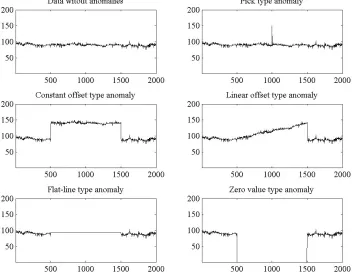
To assist in the process of anomaly detection, a framework for data validation grading and anomalous data improvement is created and presented in this paper. The proposed framework cannot provide the answer why the anomaly has occurred, but it tries to detect data anomaly and if possible, try to improve data quality. Some major anomalies, or their signatures which are possible to detect using the framework are presented in Figure 1.
related to the measurement equipment setting. Beside presented anomaly types, the signal noise corruption can also be registered as a data anomaly.
Fig. 1. Types of measurement data anomalies
After data sampling, the only remaining evidence about the captured hydro-meteorological phenomenon are data series. Despite the laboratory experiments, where the measurement process can be repeated under controlled conditions, field measurements are performed in real time with no (or with just a limited) possibility to repeat the measurement. If the data is corrupted by anomalies the only way to improve the data's reliability and quality is to use the sophisticated software tools for data validation, followed by the data reconstruction and adjustment. There is a number of data validation methods presented in the literature (Fry 2007;
Venkatasubramanian et al., 2003abc; Patcha et al. 2007; Du et al., 2006; Hill et al., 2007;
Bertrand-Krajewski et al., 2000;Branisavljević et al., 2009;Fletcher and Deletić 2008;Mourad
et al., 2002), but unfortunately, there is no universal one that can cover all the aspects of data irregularities. The main contribution of framework that is presented in this paper is the availability to apply various methods in one data validation and improvement procedure, despite majority of attempts to apply only one method.
be extended as additional information becomes available. Also, interpolation and data adjustment rely on additional information that has to provide the guidelines about the most effective methods that can be used.
In this paper a data quality improvement framework is presented that can be used for any measured variable. The framework is designed according to the three main objectives: 1) the list of data improvement methods can be extended anytime, 2) the data improvement methodology has to be adjusted for every single measured variable according to the information that is available and 3) the procedures can be used either in automatic, semi-automatic or manual mode. In order to have a flexible framework, it has to be divided into the three different data processing modules: 1) data validation module, 2) data reconstruction module and 3) data adjustment module. Of course, the presented framework is support with a appropriate database and data manager, responsible for data import and export.
Data validation is the process of data quality determination. Its main goal is to provide adequate data quality grades for data values that represent the data reliability. The framework allows the usage of several validation methods for each measured data. Each method will produce its own validation grade. The special method for grades interpretation will use all those validation grades and generate one final grade. The second module is data reconstruction. In this module, missing data and data with low quality grades are reconstructed in order to improve their reliability. Some analytical interpolation techniques are presented in this paper, but the methodology is far more broad (classification, clustering, etc.). This module is designed to use the redundant data or data with higher validation grades in order to reconstruct the data with lower grades. At the end of the improvement process, the data adjustment provides the adequate data form that is suitable for specific users, models or directly for the decision-makers. Noise reduction, statistical processing, re-sampling etc. are just some of the methods that can be used within data adjustment module of the presented framework.
After the completion of the data improvement process data values are equipped with the universal meta-data that represents the history of validation and data reconstruction. The genuine data is stored too, to allow for later framework reuse in manual mode, with different settings of the same methods or with new, improved methods. Finally, the adjusted data for different users is also stored, to keep a track of data versions and different users.
2. Measured data quality and reliability
Hydro-meteorological data is usually gathered and organized in specialized databases called Hydro-informational systems (HIS). Major role in the HIS reliability and usability takes the data quality assessment and improvement process. This process has to be performed before the data is distributed to the end user, no matter whether the end user is a computer program or an expert.
There is a variety of methods studied and presented in the literature that deal with the data quality, both of its assessment and improvement (Fry 2007; Venkatasubramanian et al.,
2003abc; Patcha et al. 2007;Du et al., 2006;Hill et al., 2007; Bertrand-Krajewski et al., 2000;
Branisavljević et al., 2009;Fletcher and Deletić 2008;Mourad et al., 2002), but, despite some
attempts (Mourad et al., 2002), it can be noticed that there is a lack of general methodology. There are several definitions of data quality that can be found in the literature:
1. GIS Glossary: Data Quality refers to the degree of excellence exhibited by the data in
2. Government of British Columbia: The state of completeness, validity, consistency, timeliness and accuracy that makes data appropriate for a specific use.
3. Glossary of Quality Assurance Terms: The totality of features and characteristics of
data that bears on their ability to satisfy a given purpose; the sum of the degrees of excellence for factors related to data.
4. Glossary of data quality terms published by The International Association for
Information and Data Quality (IAIDQ): the fitness for use of data; information that meets the requirements of its authors, users, and administrators.
5. Data quality: The processes and technologies involved in ensuring the conformance of
data values to business requirements and acceptance criteria.
Data quality directly indicates data reliability and therefore influences the decision-making. Decision- making is the process where, according to some information, experience or intuition, one among various solutions is chosen. The data quality is, therefore, directly related to decision quality. The term “decision quality” implies that decisions are defensible (in the broadest scientific and legal sense). Ideally, decision quality would be equivalent to the correctness of a decision, but in the environmental field, decision correctness is often unknown (and perhaps unknowable) at the time of decision-making. When knowledge is limited, decision quality hinges on whether the decision can be defended against reasonable challenge in whatever venue it is contested, be it scientific, legal, or otherwise. Scientific defensibility requires that conclusions drawn from scientific data do not extrapolate beyond the available evidence. If scientific evidence is insufficient or conflicting and cannot be resolved in the allotted time frame, decision defensibility will have to rest on other considerations, such as economic
concerns or political sensitivities(Crumbling, 2002).
Therefore, many factors that have impact on data quality have impact on decision making. Despite the lack of knowledge, economic or political arbitrage, if the decision only depends on measured data series, there are three scopes that have to be paid attention on if one wants to determine data quality. Measuring process has to be covered according to three scopes:
Technical scope,
Expert's scope and
Relation-based scope
Technical scope covers the technical issues about the measurement implementation (sensor characteristics and behavior, data logging and transmission, data warehousing, etc.). Expert's scope covers the issues associated with the measurement environment (variables that are measured, operational characteristics of the monitored system, characteristics of the phenomenon that is captured, etc.). Relational scope cover the issues that are related to the relations between the variables monitored (statistical relations, physical relations, logical relations, etc.).
There is number of examples of data quality assessment and improvement in the scientific literature (Fry 2007, Patcha et al. 2007, Du et al. 2006, Hill et al. 2007, Bertrand-Krajewski et
al. 2000. Branisavljević et al. 2009, Mourad et al. 2002). However, the documents that are
operation of measuring devices, their physical relation with the measured variable, calibration principles and basic and advanced principles of digital signal processing. In addition to this some factors that have an influence on data quality are specified:
Grade about the issue whether the system can fulfill the requirements regarding data quality, technical and functional characteristics. This factor covers a wide range of measurement system characteristics that is crucial for performing good measurement practice (from legislative to human resources):
Proper selection of measurement equipment,
Installation procedure and the proper working conditions,
Measuring equipment compatibility,
Micro-location and proper position of measuring equipment (especially sensors),
Proper tuning of the sensors (e.g. averaging),
Data acquisition procedure,
Data processing,
Real-time quality control,
Performance monitoring,
Testing and calibration,
Maintenance,
Training and education and
Meta-data quality.
Each of the itemized factors can significantly influence measured data and reduce its quality. If possible, after an anomaly was detected in data detection it is necessary to provide an isolation of the factor that produced the anomaly, and to adequately react.
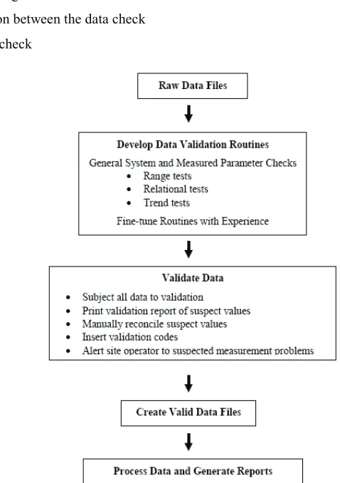
Beside this WMO's manual, a number of specialized manuals for data quality management can be found in the literature. In general, those manuals contain detailed instructions on how to calculate the indicators of the data quality, mostly by statistical means. The procedure for wind measurement data quality assessment (Fundamentals for conducting a successful monitoring program, 1997) is presented here as an example. In this practical study, beside some guidelines for installing and tuning the equipment for the wind speed measurements, a clear procedure and algorithms for data validation, data quality assessment and reconstruction of measured data values are given. Data validation process as proposed by this study can be presented in the form of the diagram shown in Figure 2.
1. Data screening
a. number of data checks (check whether there are enough values data in the series)
b. missing data gaps localization
2. Data validation
a. data range check
b. relation between the data check
c. trend check
Fig. 2. Data validation procedure, according to (Fundamentals for conducting a successful monitoring program, 1997)
The framework presented in this paper provides broad support for presented type of data validation algorithms. The support is organized in combining validation methods and providing the validation grade for every single data value.
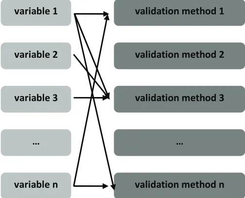
The main reason for the development of the general framework for hydro-meteorological data quality assurance and improvement was the goal to integrate the number of validation methods with powerful data management infrastructure. Such framework could be adaptable to various measured variables, allowing easy customization while keeping the same general layout. Since the applicability of validation methods lays in the availability of additional information, and since each measured data value can be processed with a number of validation methods, the framework will allow for the design of the optimum validation procedure for every single measured variable and will support the usage of other related or redundant data. The applicability of validation methods on certain measured variables is schematically presented in Figure 3.
Fig. 3. Scheme of validation method applicability
3. Increasing reliability of measured data
Data quality assessment and improvement framework is presented on Figure 4. The three successive steps of this process are clearly separated: data validation, data reconstruction and data adjustment according to user needs. Data manager, which communicates with databases and transfers the data between the validation, reconstruction and adjustment modules, is presented as arrows and is an important part of the system.
Data validation is the first step in the process of data quality improvement. To make efficient data reconstruction and data adjustment possible, data validation module (Figure 4) has to be able to produce some information about the data quality and reliability. Validation scores, which may be either binary (zeroes and ones), continuous (0-100%), or descriptive (good, uncertain or bad), are the results of the operation of the data validation module. The original data time series and the data validation scores (stored as meta-data) are the input variables for the data reconstruction module.
The operation of the data validation module follows the operation of the data reconstruction module. In the data reconstruction module, missing data and data with low quality grades are substituted by the more reliable ones, if possible. Various techniques, like data interpolation, usage of redundant data, etc. can be used manually, semi-automatically or automatically.
variable 1
variable 2
variable 3
…
variable n
validation method 1
validation method 2
validation method 3
…
D a ta Va lid atio n
Online
O ff-line real-tim e
O ff-line
D ata R e co ns truc tio n
D ec ision syste m
D ec ision syste m R econstruc tion
procedures
D ata adjus tme nt procedures Ev aluati on o f r ec on str uc tio n r esu lts Eva lua tion o f f ilte rin g r esu lts
D a ta A d jus tm e nt
Ti m e se rie s Ti m e se rie s Ti m e se rie s Va lid atio n s cor es Sc ore s Sc ore s A ddi tio na l da ta Te m po rar y da taba ses
D a ta ba se s
lin ea r
i nter p . low -pas sfilters
sp line
i nter p . high-passflitlers
...
...
regress ion bas ed
w a velet bas ed
c orrela tion bas ed
regress ion bas ed
Fig. 4. Data quality improvement framework
After data reconstruction, the module for data adjustment has to adjust and transform data in order to make it more suitable for further use. Data re-sampling, filtering and statistical calculations are just some of the techniques that if required can be accomplished in this module. After all three modules, data may be transferred to the warehouse database with the meta-data (complete history) about the transformation that the data values have underwent and its quality grade that will indicate the data reliability for the future user.
The methodology for data validation, reconstruction and adjustment presented in this paper, includes the usage of available methods as a part of the whole data quality improvement framework. The mixture of different score types obtained by validation methods are combined and interpreted using both manual (expert's) and automatic (statistical or artificial intelligence) approach. The final validation scores are at the end of the process attached to the genuine datasets as new metadata and can be used in further data quality improvement steps. Also, data reconstruction and adjustment modules can be designed to act as decision-support systems that can work under expert's supervision or as totally automatic procedures, tuned to work independently from the operator (expert).
4. Data validation
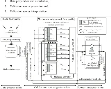
Data validation is a complex process that can be performed automatically, semi-automatically or manually with the assistance of various statistical, logical or relational tools (Figure 4). Several validation tools (or validation methods) are applied in order to assess the quality of each data value. All applied validation tools will result in validation scores that have to be interpreted and one, the final score should be created. The interpretation, based on dimensionality reduction, can be performed either by an expert (manually), by statistical tools and artificial intelligence (automatic), or by expert with a help of statistical tools and artificial intelligence (semi-automatic). For online data quality assessment the use of the automatic data validation is the only choice, while for historic data preparation or delicate phenomenon interpretation the semi-automatic or manual data validation, with the use of data visualization techniques can be used.
1. Data preparation and distribution,
2. Validation scores generation and
3. Validation scores interpretation.
Data as sim ilation
D ata v ali da tio n p re -p ro ce ss in g Warehous e D a tabas e
O nline da ta us age
M1
M... s co re
Mi sc ore
Mj sc ore
M... s co re
Mi+1 s co re
Mi+2 s co re
Mi
Mj
M2
Mi+1
Mi+ 2
...
...
...
Online or offline validation sc ore s generation
VAL IDA TI ON S COR ES Va lida tion s cor es m et a-da
ta Dep
end en t m ethod s In de pe nde nt m et hod s
M ethods O N/OFF
Valid atio n m eth o d w ith ad e q u ate d ata p re -p ro ce s sin g
L EG E ND
M eth o d tu n ing an d calib ra tio n Pr e-p r o ces sin g c on f ig u r atio n
M o d e sw itch e s
Pa ra m et er ad ju st m en t E xpert
A rtific ial intelligenc e M1
D a ta flo w p ath M eta data or igin a nd flo w p ath
Sc ore fe ed ba ck
A djustm ent of m ethods D ata pre-proces sing
Data as sim ilation
D at a ex tra ct io n an d di str ib ut io n D at a va lid at io n p re -p ro ce ss in g Warehous e D a tabas e
O nline da ta us age
M1
M1 s co re
M2 s co re
M... s co re
M... s co re
Mi sc ore
Mj sc ore
M... s co re
Mi+1 s co re
Mi+2 s co re
Mi
Mj
M2
Mi+1
Mi+ 2
... ... ... H ig h pr ior ity m etho ds VAL IDA TI ON S COR ES
M ethods O N/OFF
S c o re s in terp re tatio n Va lid atio n s core s g e n e ra tio n
D ata p rep a ratio n
Valid atio n m eth o d w ith ad e q u ate d ata p re -p ro ce s sin g
L EG E ND
Pa ra m et er ad ju st m en t R es ults E xpert
A rtific ial intelligenc e M1
D a ta flo w p ath
Sc ore fe ed ba ck
Valid atio n s c or es in ter pr etati on
A djustm ent of m ethods
A dj us tm ent of p re -pr oc es si ng
D ata pre-proces sing
Fig. 5. Data validation procedure
Step 1: Data preparation and distribution
The procedure starts with data collection and assimilation from different sources, as well as the basic data pre-processing that includes data normalization, simple data check (e.g. “is data value a numeric value?”) and data storing in relational database. From a relational database, the data manager should distribute the data and their existing meta-data “on-demand” to the data validation modules and transfer the calculated validation scores back to the database as new meta-data.
Step 2: Validation scores generation
In this part of the data validation system, the data is transferred to validation methods that generate validation scores according to the specific logic and available information. The general data pre-processing should precede the score generation in order to adjust the data according to the each method’s needs, configurations and settings. At this stage, the data pre-processing should not produce any judgment about the data quality. It has just to prepare the data for the efficient use by succeeding data validation methods. More detailed description of this step is given in the forthcoming text.
Step 3: Validation scores interpretation
(meta-data) of examined data. There are three different ways to do that: manually, semi-automatically or automatically. The anomaly detection result (score in the form of meta-data) can be discrete or continuous.
The numerous tools and methods are used in engineering practice and scientific work in order to provide the answer to a quite simple question: “Is the considered data value anomalous or not?” However there is no perfect or universal tool for anomaly detection. The successfulness of the tool applied depends on a number of factors. Some of these factors are: the type of the monitored variable, overall measuring conditions, sensor/monitoring equipment used, characteristics of the captured phenomenon, etc. Validation tools usually have several validation methods while each method can have its own specific pre-processing needs to increase the speed of operation and the overall performance.
One cluster of validation methods that can be applied in a manual, semi-automatic and automatic validation procedure is presented in Figure 6. Usually, the performance is better if the methods are used manually or semi-automatically, but sometimes satisfactory results may be accomplished in the automatic mode. Data has to pass the general pre-processing part before entering the chain of data validation methods. Checking time scale consistency, generation of additional temporary time series with different time step using different interpolation or aggregation techniques or data labeling according to the additional information acquired (day or night? pump on/off? rainy or not? etc.) are some of the actions that can be performed to increase efficiency of data transfer and processing by the main part of data validation process – validation score generation by validation methods.
Data validation methods have to be properly implemented. Implementation depends both on method design and method position in the system. There are three categories of validation methods that have a special position in the system (Figure 6): high-priority methods that are applied successively, dependent methods that depend on the results of high-priority methods and independent methods. High-priority methods have to be applied at the start of the system and their role is twofold. They have to provide data validation grades according to its (method's) logic and to prepare data for the application of dependent methods.
The validation methods are prepared to communicate between each other (communication is specified by validation structure). In this way, one method can influence the operation of its succeeding method, or it can adjust and store its own parameters for the next method run. Using those features, the framework supports the self-adjustment and feedback. Also, using the additional self-learning methods the behavior of experts during validation process can be mimicked. During the off-line usage of the framework, the expert can check the behavior of the self-learning system and self-adjusting process, and can correct them.
In order to a have properly designed validation system it is necessary to cover all the specified time series characteristics. That's why it is necessary to provide proper knowledge base about all the aspects that influence the measuring process and available data validation tools and additional information. There are a number of tools available for data validation. They can be divided into several groups:
Visualization based tools,
Statistical tools (univariate and multivariate),
Relational based tools (qualitative and quantitative models) and
M1
M2
M... s co re
Mi sc ore
Mj sc ore
M... s co re
Mi+1 s co re
Mi+2 s co re
...
VA
LI
DA
TI
O
N S
COR
ES
D ep e n den t m eth o d s
In d e pe n d en t m eth o d s
D at a va lid at io n p re -p ro ce ss in g
M1 s co re
M2 s co re
M... s co re
M... s co re
Mi sc ore
Mj sc ore
M... s co re
Mi+1 s co re
Mi+2 s co re
Mi Mi+1 Mi+2 Mj ... ...
VA
LI
DA
TI
O
N S
COR
ES
D
at
a
H ig h p rio rity m eth o d s
Fig. 6. Validation scores generation – methods topology
The first group of tools represents the traditional methods for data validation and error detection. Detection of zero values, values with flat line anomalies, values exceeding the absolute minimum or maximum or power supply failure are some of the anomalies that are easy to recognize by the visual check by an expert. The second category of anomaly detection tools contains methods based on the assumption that observed data follows some statistical laws. In univariate statistical tools it is assumed that the data follows some statistical distribution and the multivariate statistical tools are based on dimensionality reduction based mostly on data correlation. The third category of anomaly detection tools contains methods that are based on relations between the data values. Quantitative models are usually based on the threshold of allowed difference between the expected values from the model and the measurement. Qualitative models are more descriptive ones. They are usually defined as weak relationships based on common sense, logic and physical laws. The fourth group, the data mining tools are techniques and methods that have the common task to extract knowledge from the huge sets of data. Clustering, classification, vector quantization or feature extraction are some of them.
4.1 Examples of validation methods
Examples of univariate statistical methods
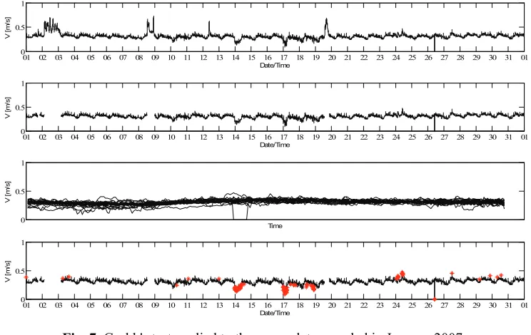
In Figure 7 the time series of measured velocities at the outlet of a combined sewer in Belgrade is presented. The velocities are measured by the ultrasonic device with a time step
t=5minutes. It is assumed that the velocities are following the Normal distribution during the
dry period, if the data sets are sampled at a certain time during the day (one data sample consists of all the data about the velocities at certain time). Since the seasonal effect is present, only the amount of data corresponding to one month is processed at the time.
After removing the data that are recorded during the runoff period (the data is separated using the additional information about the days with a rainy and dry weather) it is assumed that
the data ordered by time follows the Students t distribution, with (N-2) degrees of freedom and
the (/2N) significance level (=0.05). It should be noticed that N is the number of values in
data sets. The size of data sets is not the same for all sets (some of the data values are excluded and some are missing) and the maximum size of a data set is 31 (the month of January has 31 days). For this analysis the Grubb's test is used in several iterations. In a single iteration one outlier is rejected according to the following statistics:
Fig. 7. Grubb's test applied to the sewer data sampled in January 2007.
2 /(2 ), 2
2 / (2 ), 2
1 2
N N
N N t
N G
N t
N
(1)
where:
max
Y Y
G s
(2)
The measurement space is transformed into the G statistic feature test and the decision
space is based on the threshold value calculated on the Student’s t distribution with (N-2)
degrees of freedom. The extended Grubb's test which provides more than one outlier in single iteration is called Rossnan's test. The Z score test, Q test, Dixon test, etc. are also based on a similar logic (Venkatasubramanian et al. 2003a).
01 02 03 04 05 06 07 08 09 10 11 12 13 14 15 16 17 18 19 20 21 22 23 24 25 26 27 28 29 30 31 01 0
0.5 1
Date/Time
V
[m
/s
]
01 02 03 04 05 06 07 08 09 10 11 12 13 14 15 16 17 18 19 20 21 22 23 24 25 26 27 28 29 30 31 01 0
0.5 1
Date/Time
V [
m
/s
]
0 0.5 1
Time
V
[m
/s
]
01 02 03 04 05 06 07 08 09 10 11 12 13 14 15 16 17 18 19 20 21 22 23 24 25 26 27 28 29 30 31 01 0
0.5 1
Date/Time
V
[m
/s
Beside the presented test, based on the special data ordering so that the data can be represented by the Normal distribution, various statistical methods may also be used with the data acquired using hardware redundancy. Usually the task of data validation is extended to data fusion since the data is collected according to different (but similar) conditions and one has to find the representative value for the measured process.
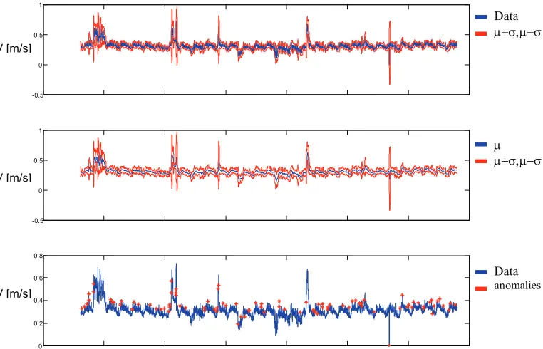
Statistical methods can be extended and based on the moving window statistics. The moving window represents a subset of time series that slides along the timeline. If it is assumed that the changing rate of the time series is small and the noise corruption is moderate, then the anomalies may be captured by comparison of some dispersion measure (standard deviation) of the moving window set of values to the one of the original values in the moving window. This method, for example, may be used for the detection of sudden spikes in the smooth time series, Figure 8.
Fig. 8. Moving window method for anomaly detection
Multivariate statistical tools
Usually there is more than one measured variable in the monitored process. Sometimes the number of measured variables is so great that it is difficult to introduce all of them to a comprehensive data analysis. However, not all the measured variables are significant for the monitored process. The multivariate statistical methods have a double role: 1) to extract the significant variables based on relations between the variables and 2) to use the existing relationships to extract the information relevant for the data validation.
In recent years the Principal Component Analysis (PCA) became a very popular method for multivariate statistical analysis (Venkatasubramanian et al. 2003a). PCA is a method based on the decomposition of the measurement correlation matrix by singular value decomposition. The core of this method is the transformation of measurement space into the coordinate system that is selected according to the course of the largest data diversity.
V [m/s]
-0.5 0 0.5 1
-0.5 0 0.5 1
0 0.2 0.4 0.6 0.8
Data
Data
anomalies
V [m/s]
Fig. 9. PCA fitting the data into the coordinate system based on the largest data diversity (pc#1, pc#2 and pc#3 are principal components)
The PCA is based on transforming the data set X into a linear matrix system based on the
correlation matrix of matrix X:
T a
X TP E (3)
where X is original data set [m x n] where n is number of variables and m is number of values
available for fitting the model. T is called the score matrix [m x a] and it contain values
transformed according to the new coordinate system based on maximum data correlation. P,
with dimension [a x n], is called the load matrix and it represents the transformation matrix. E
is the model residual (noise). The dimension that appears in matrices T and P is the number of
so-called principal components - the major coordinates of a system based data diversity. When the model is defined based on regular data set it is possible to formulate a powerful method for
data validation based on PCA. Usually, the Hotelling's t2 statistics (the generalization of
Student's t distribution for multivariate statistics) is used for the residual generation based on the
PCA model:
2 ( )T ( )
t n x
W x
(4)where n is the number of data samples, x the data sample, m the mean of data samples and W
the covariance matrix of a data sample. If the t2 statistics does not belong to a certain interval
based on the threshold value, the data may be considered anomalous.
Unfortunately, the PCA is based on correlation matrix that represents linear relations. Since the environmental data usually follows nonlinear relationships and trends, the PCA sometimes may give poor results. To extend the method to nonlinear relations there is number of attempts, but so far none seems to be superior to the others.
Beside the rough error detection, visualization is also used for detection and confirmation of the existence of the relations among data values. The relationships mainly fall into the following two categories:
known physical relationships and
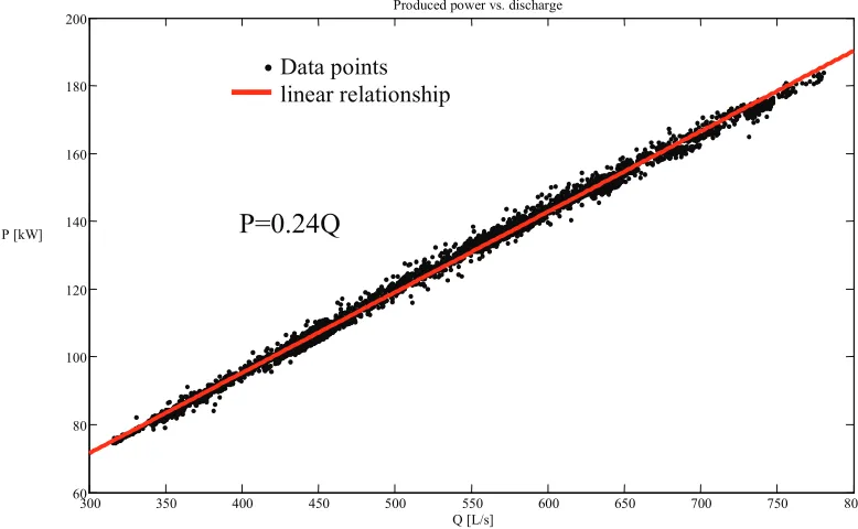
The known physical relationships are confirmed and parameters are calibrated upon the visual inspection. In Figure 10 an example of a known relationship between the discharge and the produced power of the one of the turbines in the “Iron Gate 1” HPP is presented.
Fig. 10. An example of a relation between the turbine discharge and the produced power
This relation is based on the equation P = ρ·g·HT·Q· , where P is the power, -
efficiency, ρ – specific density of water, HT – difference between water levels upstream and
downstream of the dam and Q is the discharge. Since this relation is not very sensitive to the
difference in water levels, only the relation between the power and the discharge is used. In certain cases the statistical relationship can be determined depending on a certain physical or logical conclusion. In Figure 11 a region of the upstream water level and the discharge through the turbines is emphasized, since a certain discharge can appear only with when a sufficient water head exists. Any data value that is outside of specified region can be marked as anomalous.
It is desirable to have a redundant coverage of a certain characteristic by different methods. The redundancy, either explicit (with the two sensors for the same quantity) or implicit (using simple numerical calculations) can improve the validation success. Using the redundant data the certain characteristic can be checked using different validation methods and different procedures.
300 350 400 450 500 550 600 650 700 750 800
60 80 100 120 140 160 180 200
Q [L/s] P [kW]
Produced power vs. discharge
Data points linear relationship
.
Fig. 11. Example of a visually determined region
5. Data improvement - reconstruction
After data validation, data values are equipped with the validation scores. The next step in the procedure for improvement of data quality is data reconstruction. Data reconstruction is a process of filling gaps in the time series, originated due to not sampled values and values with low validation scores. If the validation scores used in data validation process have the binary form (0 for regular data and 1 for anomalous data), all the data with validation scores equal to 1 (anomalous ones) has to be reconstructed with missing data values (data values that are not sampled). If the validation grade interval is continuous, a certain threshold value must be provided to distinguish the anomalous data from the regular one.
The data reconstruction procedure is divided into the three steps: 1) data gaps isolation, 2) provision of suitable method for data reconstruction and 3) data interpolation. Four data reconstruction methods are available: 1) model-based interpolation, 2) nearest-neighbor interpolation, 3) linear interpolation and 4) polynomial interpolation.
Model based interpolation is based on the detected relations and determined during visual inspection of data. It must be emphasized that since the models are formed only for certain variables, only some of the variables can be reconstructed by this method. Nearest-neighbor interpolation is suitable for small data gaps and time series with small resolutions. For example, this type of data reconstruction is applied on time series of the upstream water levels (Figure 12 – upper diagram). Linear interpolation is the most common method of interpolation used in data
reconstruction. In linear interpolation, two boundary data points ([xa,ya] and [xb, yb]) are used
for data approximation in between them:
b a
a a
b a
y y
y y x x
x x
(5)
0 200 400 600 800
time
Q [
L
/s
]
Discharge
68.5 69 69.5
time
Z [
m
]
Water level in accumulation
68.50 68.6 68.7 68.8 68.9 69 69.1 69.2 69.3 69.4 69.5
200 400 600 800
Z[m]
Q [
L
/s
]
Water level vs. discharge
Linear interpolation can be used on small and medium data gaps in data series that are smooth even with noise present. In the case of the time series with the abrupt changes in values (e.g. discharge through turbine, turbine power, etc.) linear interpolation can be applied
automatically only if there is no substantial difference between the boundary data points ya and
yb:
2
a b
y y u (6)
where u is a value that corresponds to data uncertainty. If this inequality does not hold, the
applicability of linear interpolation has to be verified by visual inspection, or a predefined relationship if one exists. Polynomial interpolation is used on large data gaps in smooth data series. Only interpolation based on a second degree polynomial can be used for filling of the gaps with monotonic data series, since the polynomials of a different degree are not monotonic. The polynomials of a higher degree were not used in present analysis. To verify the reconstruction performed by the means of the polynomial interpolation, a visual check must be performed.
Fig. 12. Interpolation on various time series (red lines)
6. Data adjustment
Data adjustment is a technique to optimize the data for a specific user. Thus, the validated and reconstructed data are unique, while adjusted data becomes just one of the possible versions of data, suited to the optimum specific usage (for usage in certain simulation models, for example). Data adjustment procedures can be categorized as: 1) provision of statistical information about data, 2) data filtration and 3) data re-sampling and aggregation.
The simplest statistical information, like the minimum, maximum or average values can be provided on daily, monthly or yearly bases. Data filtering is essential for reduction of total data volume and will also reduce the measurement noise present in the time series, if applied
69.1 69.2 69.3 69.4
time [m]
Nearest-neighbor
40.5 41 41.5
Interpolated
data
time [m]
Linear interpolation - smooth data series
0 200 400 600 800
unresolved
time [L/s]
correctly. Moving average filters are used for processing of smooth time series with no abrupt changes in value. If abrupt changes in value are present, the method of moving average is not suitable, since it minimizes the change and disturbs the moment of change. For time series with abrupt changes the moving average filter should be modified. It can have the form of a self-adaptive filter, averaging only if the boundary values in the moving window do not differ too much. The difference threshold and the size of the moving window are determined using the historical values. This method of filtering is presented in Figure 13.
Fig. 13. Filtering smooth time series and time series with abrupt changes in value
Re-sampling is a process of changing the time step used for sampling of the time series in question. Re-sampling can be performed by: 1) sampling with a specified time step from the data series or 2) calculation of values representative the for certain time step. Value representative for the certain time step can be: 1) an average value, 2) a minimum or maximum value or 3) a cumulative value. In Figure 14 are presented some examples of time series re-sampling.
Data aggregation is a term that denotes a process of combining various data instances into unique information. In the data aggregation process data can originate either from the different measuring equipment, or can be even come from the different sources.
40.6 40.8 41 41.2 41.4 41.6 41.8 42
time
[m
]
Filtering smooth data series
0 200 400 600 800
time
[L
/s
]
Filtering data series with abrupt changes
Data
Fig. 14. Data re-sampling (red - values sampled with a specified time step, green - average values, blue - minimum values, yellow - maximum values).
Fig. 15. Water levels data aggregation
In Figure 15 is presented data aggregation of 12 measured water levels in front of the intake structure of the hydropower plant “Iron Gate 1”. The representative value is calculated as the average value of the original data samples (without reconstructed ones).
450 500 550 600 650 700 750 800 850
time
[L
/s
]
Discharge values re-sampling
* Specified time step sampled data
* Average values
* Minimum values
* Maximum values
40.6 40.8 41 41.2 41.4 41.6 41.8 42
time
[m
]
Water levels aggregation
Data
7. Conclusion
In this paper a procedure for data quality assurance and improvement of the continuously sampled hydro-meteorological data is presented. Paper presents an innovative approach with general framework applicable to all data acquisition systems. The framework consists of three clear steps: 1) data validation, 2) data reconstruction and 3) data adjustment, and is supported by a versatile data management system. The proposed framework can incorporate any number of validation methods and can be easily customized according to the characteristics of every single measured variable. The framework allows for the self-adjustment and feedbacks in order to support self-learning of used validation methods, as well as expert-controlled learning and supervision.
After data validation, the quality of low scored data can be improved in data reconstruction module. By applying different interpolation techniques or using redundant data value the new data is created along with the accompanying metadata that contains the reconstruction history. After data reconstruction, the framework supports the data adjustment, a post-processing phase where the data is adjusted for the specific needs of each user. Every validated and sometimes improved data value is accompanied with a meta-data that holds its validation grade as a quality indicator for further use.
The proposed framework can be used either as an on-line procedure, implemented on a data acquisition server, and operating with only an occasional expert's check, or as off-line procedure, under control of an expert.
References
Bertrand-Krajewski JL, Laplace D, Joannis C, Chebbo G (2000), Mesures En Hydrologie
Urbaine Et Assainissement, Tec&Doc.
Branisavljević N, Kapelan Z, Prodanović D (2009), Bayesian-Based Detection Of Measurement
Anomalies In Environmental Data Series, HYDROINFORMATICS 2009., Chile
Crumbling DM (2002), In Search Of Representativeness: Evolvingthe Environmental Data
Quality Model, Quality Assurance, 179–190
Du W, Fang L, Peng N (2006), LAD: Localization anomaly detection for wireless sensor
networks, Parallel Distrib. Comput., No. 66, (2006), pp 874 – 886
Fletcher T and Deletić A (2008), Data requirements for integrated urban water management,
Urban Water Series – UNESCO IHP, Teylor & Francis.
Fry B (2007), Visualizing Data, O'Reilly Media, Inc. ISBN: 0596514557
Fundamentals for Conducting a Successful Monitoring Program (1997), WIND RESOURCE
ASSESSMENT HANDBOOK, AWS Scientific, Inc. CESTM, 251 Fuller Road, Albany, NY 12203, www.awsscientific.com, April 1997
Guide to Meteorological Instruments and Methods of Observation (2006), Preliminary seventh edition, WMO-No. 8, Secretariat of the World Meteorological Organization – Geneva – Switzerland 2006
Hill D, Minsker B, Amir E (2007), Real-time Bayesian Anomaly Detection for Environmental
Sensor Data, Proc. of the 32nd Congress of IAHR, International Association of Hydraulic Engineering and Research, Venice, Italy, (2007)
http://en.wikipedia.org/wiki/Data_quality
Kumar M, Budhathoki NR, Kansakar S (2002), Hydro-Meteorological Information System:
Mourad M and Bertrand-Krajewski JL (2002), A method for automatic validation of long time series of data in urban hydrology. Water Science and Technology Vol 45 No 4–5 pp 263– 270 © IWA Publishing
Patcha A and Park J (2007), An overview of anomaly detection techniques: Existing solutions
and latest technological trends, Computer Networks, No. 51, (2007), pp 3448–3470
Venkatasubramanian V, Rengaswamy R, Yin K, Kavuri S (2003a), A review of process fault
detection and diagnosis Part I: Quantitative model-based methods, Computers and Chemical Engineering, No. 27, (2003), pp 293-311
Venkatasubramanian V, Rengaswamy R, Yin K, Kavuri S (2003b), A review of process fault
detection and diagnosis Part II: Qualitative models and search strategies, Computers and Chemical Engineering, No. 27, (2003), pp 293-311
Venkatasubramanian V, Rengaswamy R, Yin K, Kavuri S (2003c), A review of process fault
detection and diagnosis Part III: Process history based methods, Computers and Chemical Engineering, No. 27, (2003), pp 293-311