RELIABILITY AND FUZZY ANALYSIS OF A SYSTEM HAVING THREE UNITS

Seema. World Journal of Engineering Research and Technology

RELIABILITY AND FUZZY ANALYSIS OF A SYSTEM HAVING

THREE UNITS

Dr. Seema Sahu*

Assistant Professor (Computer Science), BCS Govt. PG College, Dhamtari (C.G.).

Article Received on 23/05/2018 Article Revised on 13/06/2018 Article Accepted on 04/07/2018

ABSTRACT

This paper presents a reliability analysis of a system having three units.

The first step in the proposed methodology is assumption of model.

Second step involves calculating Transition Probabilities, Mean Time

to system failure, Availability analysis, Busy Period Analysis. Third

step is to take particular Cases using fuzzy logic and Erlangian

distributions. Fourth step is to calculate profit analysis and defuzzify the fuzzy profit analysis

by using signed distance ranking method for defuzzification. It helps to allocate reliability of

model before the actual system is built. It also helps to estimate the exact value of profit.

KEYWORDS: Triangular Fuzzy Number, MTSF, Availability, Busy Period, Signed Distance Ranking Method.

1. INTRODUCTION

In the present generation functional reliability of machines is top priority for system

managers and they are in dire need for such system which is fault free. Reliability analysis

provides an opportunity for keeping the system fault tolerant and it is vital for proper

utilization and maintenance of any system. Reliability analysis basically involves having

standby redundant system and timely maintenance of whole system. This technique helps for

increasing system effectiveness through reducing failure and cost minimization. Standby

redundant systems represent one approach to improving system reliability. Spare parts and

back systems are examples of standby redundancy. Barlow and Prochan,[1] carried our pioneer work in the field of Reliability and Life Testing of Probabilistic models. Then on,

World Journal of Engineering Research and Technology

WJERT

www.wjert.org

SJIF Impact Factor: 5.218

*Corresponding Author Dr. Seema Sahu

Assistant Professor

(Computer Science), BCS

Govt. PG College, Dhamtari

redundant system with parallel configuration was discussed by the likes of Osaki.[2] Chandrasekhar et al[5] performed the same study taking the Eglangian distribution in repair time. In recent years various reliability models have been formulated for predicting,

estimating or optimizing the probability of survival, the mean life or more generally the life

distribution of components or systems. Industries are trying to develop more and more

automation in their industrial processes in order to meet the ever increasing demands of

society. The complexities of industrial systems as well as their products are increasing day by

day. A parallel work in this field was done by Rander[3] by performing analysis of cold standby system with preventive maintenance and replacement of standby unit. Singh et al[6] studied reliability characteristics of an integrated steel plant. This kind of analysis is of

immense help to the owners of small scale industry. Also the involvement of preventive

maintenance and replacement of standby unit in the models increase the reliability of the

functioning units to great extent. At last fuzzy technique is used to assess the cost of the

2. Definitions and Preliminaries

A fuzzy set A is defined by a membership function µA(x) which maps each and every element of X to [0 1] i.e.,

µA(x)  [0 1] [2.1]

where, X is the underlying ground set. In simple, a fuzzy set is a set whose boundary is not clear. On the other hand, a fuzzy set is a set whose elements are characterized by a

membership function as above.

The - cut of a fuzzy set A is the crisp subset of the ground set X, that contains all the elements whose membership grade is greater than or equal to . It is denoted by A and is defined by

A = x µA(x)  , xX} [2.2]

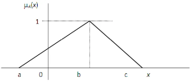
A triangular fuzzy number is a fuzzy set. It is denoted by A = (a,b,c) and defined by the following membership function

  

    

    

  

 



c x

c x b b c

x c

b x a a b

a x

x a

x

A

; 0

; ; ; 0

) (

 [2.3]

where, a, b, c  R, A FN where FN is the set of triangular fuzzy numbers and is represented graphically as

Properties of triangular fuzzy numbers

If A & B are two fuzzy numbers then their sum is also a fuzzy number. Suppose A = (a, b, c) & B = (u, v, w) then,

) , , ( ) , ,

(a b c u v w B

A  

= (au,bv,cw)

) , , ( ) , ,

(a b c u v w B

A  

= (a,b,c)(w,v,w)

= (aw,bv,cu)

Example: Let A = (-2, 2, 3) & B = (-1, 0, 4) AB(1,2,3)(1,0,4)

= (21 ,20,34)

= (3,2,7)

AB(2,2,3)(1,0,4)

= (2,2,3)(4,0,1)

= (6,2,4)

Def 1: - Let d*(c, 0) = c; c, 0  R

Geometrically, c>0 means that c lies to the right of the origin O and the distance between c

and O is denoted by c = d*(c, 0). Similarly, c<0 means that c lies to the left of the origin O

and the corresponding distance between c & o is denoted by –c = d*(c, 0). Therefore, d*(c,

O) denotes the signed distance of c which is measured form O.

Def 2:- Signed-distance for A = (a, b, c) FN, a triangular fuzzy number, the signed-distance of A measured from O~₁is defined by

d (A, 1

~

O ) = ( 2 )

4 1

c b

a 

Def 3:- Let A=(a, b, c) & B = (u, v, w)  FN. Then the ranking of fuzzy numbers on FN is defined by

B

A iff d (A, O~₁) < d (B,O~₁) & AB iff d (A, 1

~

O ) = d (B, 1

~

Fuzzy number are fuzzy subsets of set on real number satisfying some additional condition.

Fuzzy number allow us to model non-probabilistic uncertainties in an easy way. Triangular

and Trapezoidal fuzzy numbers are commonly used. Therefore here I am discuss about these

two numbers only. Triangular and Trapezoidal fuzzy numbers can represented by (a, b, c) and

(a, b, c, d) respectively. Triangular fuzzy numbers are special case of trapezoidal fuzzy

numbers when b equal c.

Let A and B be two triangular fuzzy numbers, parameterized by (a1,a2,a3) and (b1,b2,b3).

Their arithmetic can be described following

A+B=(a1+b1, a2+b2, a3+b3); A-B=(a1-b3, a2-b2, a3-b1);

A*B=(a1*b1, a2*b2, a3*b3); A/B=(a1/b3, a2/b2, a3/b1)

Let A and B be two triangular fuzzy numbers, parameterized by (a1,a2,a3,a4) and

(b1,b2,b3,b4). Their arithmetic can be described following

A+B=(a1+b1, a2+b2, a3+b3, a4+b4); A-B=(a1-b4, a2-b3, a3-b2, a4-b1)

A*B=(a1*b1, a2*b2, a3*b3, a4*b4); A/B=(a1/b4, a2/b3, a3/b2, a4/b1)

These are the operations performed on fuzzy numbers. However, these values need to be

mapped to real values for the calculation. Process of converting fuzzy numbers into crisp

numbers is called defuzzification. Formula for performing defuzzification operations on

triangular and trapezoidal fuzzy numbers. These formulas are given below. Let A(a1, a2, a3)

and B(b1,b2,b3) are two triangular fuzzy numbers. Their defuzzification formula is given as



a b c



t

G  2 

4 1 ) (

3. System Description of the model

The system consists of three units namely one main unit A and two associate units B & C.

Here the associate unit B and C are dependent upon main unit A when the system is in

operation. The system functions when the main unit and at least one of the associate units are

working. The system is taken in down mode when the main unit is not functioning. As soon

as a job arrives, all the units work with load. It is further assumed that only one job is taken

for processing at a time. There is a single repairman who repairs the failed units on first come

first served basis. Using regenerative point technique several system characteristics such as

transition probabilities, mean sojourn times, availability and busy period of the repairman are

end, profit analysis is done with the help of values of MTSF, Availability and Busy Periods

and fuzzy technique is used to calculate the actual profit.

4. Assumptions used in the model

a. The system consists of one main unit A and two associate units B and C.

b. The main unit A works with the help of associate units B and C.

c. There is a single repairman which repairs the failed units on priority basis.

d. After a random period of time the whole system goes for preventive maintenance.

e. All units work as new after repair.

f. The failure rates of all the units are taken to be exponential whereas the repair time

distributions are arbitrary.

g. Switching devices are perfect and instantaneous.

5. Symbols and Notations



j i

p Transition probabilities from S_i to S_j 

i

 Mean sojourn time at time t

0

E =State of the system at epoch t=0

E=set of regenerative states



) (t

q_ij Probability density function of transition time from SitoSj



) (t

Q_ij Cumulative distribution function of transition time from S_itoS_j 

) (t

i

 Cdf of time to system failure when starting from stateE0 Si E

 ) (t

i

 Mean Sojourn time in the state E0 SiE

 ) (t

Bi Repairman is busy in the repair at time t /E0 SiE

4 3 2 1/r /r /r

r =Constant repair rate of Main unit A /Unit B/Unit C/ Shut down state

 

/ / =Failure rate of Main unit A /Unit B/Unit C = Repair rate from P.M.

) ( / ) ( / )

( 2 3

1 t g t g t

g =Probability density function of repair time of Main unit A/Unit B/Unit C

) ( / ) ( / )

( _{2 3}

1 t G t G t

G =Cumulative distribution function of repair time of Main unit A/Unit B/Unit C

) ( / )

( 4

4 t G t

g = Pdf / Cdf of repair time of Shut down state. a(t) = Probability density function of preventive maintenance .

5 0 S

b(t) = Probability density function of preventive maintenance completion time.

) (t

A = Cumulative distribution functions of preventive maintenance.

) (t

B = Cumulative distribution functions of preventive maintenance completion time.

= Symbol for Laplace -Stieltjes transforms. = Symbol for Laplace-convolution.

6. Symbols used for states of the system r

g A

A

A₀/ / -- Main unit ‘A’ under operation/good and non-operative mode/ repair mode g

r B

B

B₀/ / -- Associate Unit ‘B’ under operation/repair/ good and non-operative mode

g

r C

C

C₀/ / -- Associate Unit ‘C’ under operation/repair/good and non-operative mode

P.M. -- System under preventive maintenance.

S.D. – System under shut down mode.

Up states:S₀ (A₀,B₀,C₀);S₂ (A₀,B_r,C₀);S₃ (A₀,B₀,C_r) Down States: S1 (Ar,Bo,Co);S4 (S.D.);S5 (P.M.)

7. Transition Probabilities

Simple probabilistic considerations yield the following non-zero transition probabilities:

1. ( ) [1 *( ₁)]

1 0

) (

01 a x

x dt t A e

p  t  





 

 

    _,

2. _{( ) [1 ( )]}

1 *

1 0

) (

02 a x

x dt t A e

p _ t _{ }





 

 

   

3. ( ) [1 *( ₁)]

1 0

) (

03 a x

x dt t A e

p 



t  



 

 

    _,

4. ( ) *( ₁)

0

) (

05 a t e dt a x

p 



t 



    

5. ( ) ₂*( )

0

2 ) (

20  



 _{ }



_

 

g dt t g e

p t ,

6. ( ) ( ) 1 ₂*( )

0

2 ) (

24    



 _{  }





_

  

g dt

t G e

p t

7.



 

 _{ }



0

* 3 3

) (

30( ) ( ) ( )

 

g dt t g e

t

p t

8. ( ) ( ) ( ) 1 3*( )

0

3 ) (

34    



 _{  }

 





 

g dt t G e

t

p t

9. p10  p40  p50 1 Wherex1   _[7.1-7.9]

And mean sojourn time are given by

10. 1 [1 ( 1)]

* 1

0 a x

x 



 ,

11. G (t)dt

0 1 1







 ,

12. 2 _1_ [1 2*()]



 g ,

13. 3 _ 1_[1 3*( )]



 g

14. G (t)dt

0 4 4









15. B(t)dt

0 5









[7.10-7.15]

8. Mean Time to System Failure

Time to system failure can be regarded as the first passage time to the failed state. To obtain

it we regard the down state as absorbing. Using the argument as for the regenerative process,

we obtain the following recursive relations.

) ( ) ( )

( ) ( )

( ) ( )

( 01 02 2 03 3 05

0 t Q t Q t  t Q t  t Q t



) ( ) ( )

( )

( 20 0 24

2 t Q t  t Q t



) ( ) ( )

( )

( 30 0 34

3 t Q t  t Q t

 [8.1-8.3]

Taking Laplace - Stieltjes transform of above equations and writing in matrix form, We get

   

 

   



 

   

 

  

 

   

 

   

 

 

 

34 24

05 01

3 2 0

30 20

03 02

~ ~

~ ~

1 0

~

0 1

~

~ ~

1

Q Q

Q Q

Q Q

Q Q

  

30 03 02 20 30

20

03 02

1

~ ~ ~ ~ 1

1 0

~

0 1

~

~ ~

1

)

( Q Q Q Q

Q Q

Q Q

s

D   

 

 

 and

) ~ ~ ~ ~ ~ ~ (

1 0

~

0 1

~

~ ~

~ ~

)

( 01 05 02 24 03 34

34 24

03 02

05 01

1 Q Q Q Q Q Q

Q Q

Q Q

Q Q

s

N    

 



 [8.4-8.5]

s

s

Now letting s0 and noting that _{ij ij}

t Q t p

Lim 



 ( ) _, we get,

30 03 20 02

1(0) 1 p p p p

D    and N₁(0) p₀₁ p₀₅ p₀₂p₂₄ p₀₃p₃₄

The mean time to system failure when the system starts from the state S₀ is given by

MTSF=

) 0 (

) 0 ( ) 0 ( )]

( ~ [ ) (

1 / 1 /

1 0 0

D N D

s ds

d T

E   _s   [8.6]

To obtain the numerator of the above equation, we collect the coefficients of relevant of

j i

m in (0) 1/(0)

/

1 N

D  .

Coeff. of (m₀₁ m₀₂ m₀₃ m₀₅) =1

Coeff. of (m₂₀) =p₀₂

Coeff. of (m₃₀ m₃₄) =p₀₃ From equation [8.6]

MTSF=

) 0 (

) 0 ( ) 0 ( )]

( ~ [ ) (

1 / 1 /

1 0 0

D N D

s ds

d T

E   _s   =

30 03 20 02

03 3 02 2 0

1 p p p p

p p

 



 



[8.7]

9. Availability Analysis

Let Mi(t)(i0,1,2)denote the probability that system is initially in regenerative state SiE

is up at time t without passing through any other regenerative state or returning to itself

through one or more non regenerative states .i.e. either it continues to remain in

regenerativeS_i or a non regenerative state including itself . By probabilistic arguments, we

have the following recursive relations

), ( )

( ),

( )

( ),

( )

( ( ) ₂ ( ) _{2 3} ( ) ₃

0 t e A t M t e G t M t e G t

M   t   t   t [9.1-9.3]

Recursive relations giving point wise availability Ai(t)given as follows:





 

5 , 3 , 2 , 1

0 0

0( ) ( ) ( ) ( )

i

i

i t A t

q t

M t

A ; A1(t)q10(t) A0(t);





 

4 , 0

2 2

2( ) ( ) ( ) ( )

i

i

i t A t

q t

M t

A ;





 

4 , 0

3 3

3( ) ( ) ( ) ( )

i

i

i t A t

q t

M t

A ;

) ( )

( )

( 40 0

4 t q t A t

A  ; A5(t)q50(t) A0(t); [9.4-9.9]

Taking Laplace transformation of above equations; and writing in matrix form, we get

/ * 3 * 2 * 0 /

* 5 * 4 * 3 * 2 * 1 * 0 6

6 [A ,A ,A ,A ,A ,A ] [M ,0,M ,M ,0,0]

q _X 

c

c

c

c

Where 6 6 * 50 40 * 34 * 30 * 24 20 * 10 * 05 * 03 02 * 01 6 6 1 0 0 0 0 0 1 0 0 0 0 1 0 0 0 0 1 0 0 0 0 0 1 0 1 X X q q q q q q q q q q q q                                   [9.9a] Therefore 6 6 * 50 40 * 34 * 30 * 24 20 * 10 * 05 * 03 02 * 01 2 1 0 0 0 0 0 1 0 0 0 0 1 0 0 0 0 1 0 0 0 0 0 1 0 1 ) ( X q q q q q q q q q q q s D                                   * 50 * 05 * 40 * 34 * 30 * 03 * 40 * 24 * 20 * 02 * 10 *

01 ( ) ( )

1q q q q q q q q q q q q



[9.10]

If s0 we get D₂(0)0 which is true

Now 6 6 * 34 * 3 * 24 * 2 * 05 * 03 02 * 01 * 0 2 1 0 0 0 0 0 0 1 0 0 0 0 0 1 0 0 0 0 1 0 0 0 0 0 1 0 0 ) ( X q M q M q q q q M s N                           

Solving this Determinant, we get

* 03 * 3 * 02 * 2 * 0

2(s) M M q M q

N    [9.11]

If s0 we get

03 3 02 2 0

2(0) p p

N    [9.12]

To find the value of D₂/(0)_{, we collect the relevant coefficient} mijin D2(s) we get

Coeff. of (m₀₁ m₀₂ m₀₃ m₀₅)1L₀

Coeff. of (m10) p01 L1 Coeff. of (m20 m24) p02 L2

Coeff.of (m30 m34) p03 L3 Coeff.f m40  p03p34  p03p34 L4

Thus the solution for the steady-state availability is given by ) 0 ( ) 0 ( ) ( ) ( ) ( _/ 2 2 * 0 0 * 0 * 0 D N s sA Lim t A Lim A S

t  

     =



   5 , 4 , 3 , 2 , 1 , 0 3 3 2 2 0 0 i i iL L L L     [9.19]

10. BUSY PERIOD ANALYSIS

(a) Busy period of the Repairman in performing Normal repair in time (0, t]

Let Wi(t) (i1,2,3)denote the probability that the repairman is busy initially with normal

repair in regenerative stateS_i and remain busy at epoch t without transiting to any other state

or returning to itself through one or more regenerative states.

By probabilistic arguments we have

) ( )

( 1

1 t G t

W  ,W2(t)G2(t),W3(t)G3(t) [10.1-10.3]

Developing similar recursive relations as in availability, we have



  5 , 3 , 2 , 1 0

0( ) ( ) ( )

i

i

i t B t

q t

B

; B1(t)W1(t)q10(t) B0(t) ;



   4 , 0 2 2

2( ) ( ) ( ) ( )

i

i

i t B t

q t W t B ;



   4 , 0 3 3

3( ) ( ) ( ) ( )

i

i

i t B t

q t W t B ; ) ( ) ( )

( 40 0

4 t q t B t

B  ; B5(t)q50(t) B0(t); [10.4-10.9]

Taking Laplace transformation of above equations; and writing in matrix form, we get

/ * 3 * 2 * 1 / * 5 * 4 * 3 * 2 * 1 * 0 6

6 [B ,B ,B ,B ,B ,B ] [0,W ,W ,W ,0,0]

q _X  _[10.10]

Where q_6x6is denoted by [9.9a] and therefore D₂/(s)is obtained as in the expression of availability. Now 6 6 * 34 * 3 * 24 * 2 * 1 * 05 * 03 02 * 01 3 1 0 0 0 0 0 0 1 0 0 0 0 0 1 0 0 0 0 1 0 0 0 0 0 1 0 0 ) ( X q W q W W q q q q s N                           

So, we get the value of this determinant after putting s0 is

) (

) 0

( 1 01 2 02 3 03

3 p p p

N    

3 3 2 2 1

1L  L  L

  

 =



1,2,3

i

i iL

 [10.11]

Thus, in the long run, the fraction of time for which the repairman is busy with normal repair

of the failed unit is given by:

) 0 ( ) 0 ( ) ( ) ( ) ( _/ 2 3 * 1 0 0 * 1 0 * 1 0 D N s sB Lim t B Lim B s

t  

     =





  5 , 4 , 3 , 2 , 1 , 0 3 , 2 , 1 i i i i i i L L   [10.12]

(b) Busy period of the Repairman in preventive maintenance in time (0, t] By probabilistic arguments we have

) ( ) (

5 t B t

W  [10.13]

Developing similar recursive relations as in 10(a), we have



  5 , 3 , 2 , 1 0

0( ) ( ) ( )

i

i

i t B t

q t

B ; B1(t)q10(t) B0(t) ;



  4 , 0 2

2( ) ( ) ( )

i

i

i t B t

q t

B ;



  4 , 0 3

3( ) ( ) ( )

i

i

i t B t

q t

B ;

) ( )

( )

( 40 0

4 t q t B t

B  ; B5(t)W5(t)q50(t) B0(t) [10.14-10.19]

Taking Laplace transformation of above equations; and writing in matrix form, we get

/ * 5 / * 5 * 4 * 3 * 2 * 1 * 0 6

6 [B ,B ,B ,B ,B ,B ] [0,0,0,0,0,W ]

q _X 

Where q_6x6is denoted by [9.9a] and therefore D₂/(s)is obtained as in the expression of availability. Now 6 6 * 5 * 34 * * 24 * 05 * 03 02 * 01 4 1 0 0 0 0 0 1 0 0 0 0 0 1 0 0 0 0 0 1 0 0 0 0 0 0 1 0 0 0 ) ( X W q q q q q q s N                           

Solving this Determinant, In the long run, we get the value of this determinant after putting

0  s is

5 5 05 5

4(0) p L

N   [10.20]

Thus, in the long run, the fraction of time for which the system is under preventive

) 0 ( ) 0 ( ) ( ) ( ) ( _/ 2 4 * 2 0 0 * 2 0 * 2 0 D N s sB Lim t B Lim B s

t  

 

 

 =



0,1,2,3,4,5 5 5 i i iL L   [10.21]

(c) Busy period of the Repairman in Shut Down repair in time (0, t] By probabilistic arguments we have

) ( )

( 4

4 t G t

W  [10.22]

Developing similar recursive relations as in 10(b), we have



  5 , 3 , 2 , 1 0

0( ) ( ) ( )

i

i

i t B t

q t

B ; B1(t)q10(t) B0(t);



  4 , 0 2

2( ) ( ) ( )

i

i

i t B t

q t

B ;



  4 , 0 3

3( ) ( ) ( )

i

i

i t B t

q t B ; ) ( ) ( ) ( )

( 4 40 0

4 t W t q t B t

B   ; B5(t)q50(t) B0(t) ; [10.23-10.28]

Taking Laplace transformation of above equations; and writing in matrix form, we get

/ * 4 / * 5 * 4 * 3 * 2 * 1 * 0 6

6 [B ,B ,B ,B ,B ,B ] [0,0,0,0,W ,0]

q _X 

Where q_6x6is denoted by [9.9a] and therefore D₂/(s)is obtained as in the expression of availability. Now 6 6 * 5 * 34 * * 24 * 05 * 03 02 * 01 5 1 0 0 0 0 0 0 1 0 0 0 0 1 0 0 0 0 0 1 0 0 0 0 0 0 1 0 0 0 ) ( X W q q q q q q s N                           

In the long run, we get the value of this determinant after putting s0 is

4 4 30 03 24 02 4

5(0) (p p p p ) L

N    [10.29]

Thus the fraction of time for which the system is under shut down is given by:

) 0 ( ) 0 ( ) ( ) ( ) ( _/ 2 5 * 3 0 0 * 3 0 * 3 0 D N s sB Lim t B Lim B s t       =



0,1,2,3,4,5 4 4 i i iL L   [10.30] c

c c

c c

11. Particular cases

When all repair time distributions are n-phase Erlangian distributions i.e.

Density function ! 1 ) ( ) ( 1     n e t nr nr t g t nr n i i i i and

Survival function



    1 0 ! ) ( ) ( n j t nr j i j j e t nr t G i

[11.1-11.2] And

other distributions are negative exponential

t t t t e t B e t A e t b e t

a( )  , ( )  , ( )  , ( )  [11.3-11.6]

For n=1 _gi(t)_rierit _, rt

i

i

e t

G ( )  If i=1, 2, 3, 4

t r t r e r t g e r t

g 1 2

2 2 1

1( ) , ( )



 _

 ,g t re r3t

3 3( )



 , rt

e r t

g 4

4 4( )

  t r e t

G _{( )} 1

1



 ,G ₍t₎ e r2t 2



 ,G ₍t₎ e r3t 3



 , G ₍t₎ e r4t 4



 [11.7-11.14]

Also                 1 05 1 03 1 02 1

01 , , ,

x p x p x p x p 2 24 2 2 20 , r p r r p              , , 3 34 3 3 30 r p r r p              , 1 , 1 1 1 1 0 r

x  

           

 1 , 1 , 1, 5 1

4 4 3 3 4 2

2  _{ }  _{ }   

r r

r [11.15-11.30]

MTSF= 30 03 20 02 03 3 02 2 0

1 p p p p

p p       ,



     5 , 4 , 3 , 2 , 1 , 0 3 3 2 2 0 0 0( )

i i iL L L L A     ,





    5 , 4 , 3 , 2 , 1 , 0 3 , 2 , 1 * 1 0 ( )

i i i i i i L L B   ,



   5 , 4 , 3 , 2 , 1 , 0 5 5 * 2 0 ( )

i i iL L B   ,



   5 , 4 , 3 , 2 , 1 , 0 4 4 * 3 0 ( )

i i iL L B   [11.31-11.35]

WhereL0 1;L1  p01;L2  p02; L3  p03;L4  p02p24  p03p34; L5  p05;

[11.36-11.41]

12. Profit Analysis

The profit analysis of the system can be carried out by considering the expected busy period

Therefore, G(t) = Expected total revenue earned by the system in (0,t] -Expected repair cost

of the failed units

Expected repair cost of the repairman in preventive maintenance -Expected repair cost of the

Repairman in shut down

) ( ) ( ) ( )

( _{2 1 3 2 4 3}

1 t C t C t C t

C _up  _b  _b  _b

 [12.1]

Where 



t

up t A t dt

0 0()

) (

 ; t B t dt

t

b 



0 1 0 1( ) ()

 ; t B t dt

t

b 



0 2 0 2( ) ( )

 ; 



t

b t B t dt

0 3 0 3( ) ( )



[12.2-12.5]

1

C is the revenue per unit time and C₂,C₃,C₄ are the cost per unit time for which the system is under simple repair, preventive maintenance and shut down repair respectively.

Apply fuzzy concept in [12.1]

) ( ~ ) ( ~ ) ( ~ ) ( ~ ) ( ~ 3 4 2 3 1 2

1 t C t C t C t

C t

G 



_up 



_b 



_b 



_b

[12.6]

Taking triangle fuzzy number

) 8 , 5 , 24 ( ~ 1 

C C~₂ (4,2,1) C~₃ (5,3,1) C~₄ (12,6,3)

819 . 0  up 

b1 0.174 b2 0.022 b3 1.151

151 . 1 * ) 3 , 6 , 12 ( 022 . 0 * ) 1 , 3 , 5 ( 174 . 0 * ) 1 , 2 , 4 ( 819 . 0 * ) 8 , 5 , 24 ( ) ( ~ _{   } t G ) 453 . 3 , 906 . 6 , 813 . 13 ( ) 022 . 0 , 066 . 0 , 11 . 0 ( ) 174 . 0 , 348 . 0 , 696 . 0 ( ) 552 . 6 , 095 . 4 , 656 . 19 (     ) 649 . 3 , 32 . 7 , 619 . 14 ( ) 552 . 6 , 095 . 4 , 656 . 19 (   ) 619 . 14 , 32 . 7 , 649 . 3 ( ) 552 . 6 , 095 . 4 , 656 . 19 (      ) 067 . 8 , 225 . 3 , 047 . 16 (    _[12.7]

Applying defuzzification using signed distance ranking method in eq. [12.7], we get

) 067 . 8 225 . 3 * 2 047 . 16 ( 4 1 )

(t   

13. DISCUSSION AND RESULT

It is seen from the table 1.1 that value of MTSF decreases with increase in the failure rate of

main unit. The same can be predicted in the case of Availability. It is also seen that with the

application of preventive maintenance technique Availability increases to some extent. The

use of fuzzy theory in profit analysis removes the uncertainty in the cost of various

parameters and gives the exact value of profit of any system.

Table 1.1: Variations in MTSF vis-à-vis Failure Rate of Main Unit.

α β γ , θ λ r3,r4 r1, r2 MTSF

0.1 0.01 0.01 0.1 0.01 0.01 51.84 0.2 0.02 0.01 0.1 0.01 0.02 46.02 0.3 0.03 0.01 0.1 0.01 0.03 30.81 0.4 0.04 0.01 0.1 0.01 0.04 25.42

Table 1.2: Variations in Availability vis-à-vis Failure Rate of Main Unit. α Β γ , θ λ r3,r4 r1, r2 Availability 0.1 0.01 0.01 0.1 0.01 0.01 125.22 0.2 0.02 0.01 0.1 0.01 0.02 97.57 0.3 0.03 0.01 0.1 0.01 0.03 46.66 0.4 0.04 0.01 0.1 0.01 0.04 35.89

Table 1.3: Variations in Profit vis-à-vis increase Failure Rate of Main Unit.

α Β γ , θ λ r3,r4 Profit

0.1 0.01 0.01 0.1 0.01 62.592 0.2 0.02 0.01 0.1 0.01 41.222 0.3 0.03 0.01 0.1 0.01 22.129 0.4 0.04 0.01 0.1 0.01 11.027

Table 1.4: Variations in Profit vis-à-vis increase Repair Rate of Main Unit.

r3,r4 η r1, r2 γ , θ λ Profit

0.01 0.01 0.01 0.01 0.1 0.981 0.01 0.01 0.02 0.01 0.1 18.273 0.01 0.01 0.03 0.01 0.1 31.752 0.01 0.01 0.04 0.01 0.1 42.826

14. REFERENCES

1. Barlow R.E. and Proshan, Statistical Theory of Reliability and Life Testing Probability

Models, 1975.

2. Osaki. A two unit parallel redundant system with bivariate exponential life. Microelectron

3. Murari K. and Goel L.R. Comparison of two unit cold standby reliability models with

three types of repair facilities. Microelectron & Reliability, 1984; 24: 35-49.

4. Rander M.C., Kumar Ashok and Suresh K. Cost analysis of two dissimilar cold standby

system with preventive maintenance and replacement of standby unit. Microelectron &

Reliability, 1994; 34: 171-174.

5. Gupta R., Tyagi P.K. and Goel L.R. A cold standby system with arrival time of server and

correlated failures and repairs. Microelectron & Reliability, 1995; 35(4): 739-742.

6. Chandrashekhar P., Natarajan R. and Yadavalli, V.S.S. A study on a two unit standby

system with Erlangian repair time. Asia Pacific Journal of Operation Research, 2000;

21(3): 271-277.

7. Singh S.K. On the estimation and computational analysis of reliability characteristics of a

merchant mill system of an integrated steel plant. Stochastic Modeling and Application,

2000; 3(1): 68-87.

8. Muller M.A.V. Probabilistic Analysis of Repairable Redundant Systems. Ph.D. thesis,

University of Pretoria, South Africa, 2005.

9. Pathak V. K., Sahu Seema, Chturvedi Riteshwari. Wind mill system having one main unit

& three associative Units. Journal of National Academy of Mathematics, 2012; 26: 35-48.

10.Pathak V. K., Mehta Kamal, Sahu Seama, Chturvedi Riteshwari. Profit analysis of a

system Having one main unit and two supporting units. International Journal Of

Engineering And Computer Science, October 2013; 2(10): 1-13.

11.Pathak V. K., Mehta Kamal, Sahu Seema, Namdeo Ashish. Comparative study of

reliability parameter of a system under different types of distribution functions. African

Journal of Mathematics and Computer Science Research, 2014; 7(4): 47-54.

12.Sahu Seama, Pathak V.K., Mehta Kamal, Namdeo Ashish. Estimate of Mean Time

Between Failure in Two Unit Parallel Repairable System. International Journal On Recent