www.theoryofcomputing.org
Online Scheduling to Minimize Maximum
Response Time and Maximum Delay Factor
∗
Chandra Chekuri
†Sungjin Im
‡Benjamin Moseley
§Received: July 28, 2010; published: May 14, 2012.
Abstract: This paper presents several online scheduling algorithms for two related perfor-mance metrics, namely maximum response time and maximum delay-factor, and also their weighted versions. The delay factor metric is new (introduced in Chang et al. (SODA’08)), while special cases of maximum weighted response time have been considered before. We study both the standard scheduling model where each arriving job requires its own pro-cessing, as well as the broadcast scheduling model where multiple requests/jobs can be simultaneously satisfied.
Motivated by strong lower bounds, we consider the resource augmentation model intro-duced in Kalyanasundaram and Pruhs (JACM’95) where the algorithm is given a machine with faster speed than the adversary. We give scalable algorithms; that is, algorithms that when given(1+ε)-speed are O(poly(1/ε))-competitive for any fixedε >0. Our main
contributions are for broadcast scheduling. Along the way we also show that the FIFO (first-in-first-out) algorithm is 2-competitive for broadcast scheduling even when pages have non-uniform sizes. We complement our algorithmic results by showing that a natural greedy
∗This paper contains and extends results that appeared in two preliminary papers [23,22].
†Partially supported by NSF grants CCF-0728782 and CNS-0721899.
‡Supported mainly by a Samsung Fellowship and partially by NSF grant CNS-0721899. §Partially supported by NSF grant CNS-0721899.
ACM Classification:C.4, F.2.2
AMS Classification:68M20, 68Q25, 68W25, 68W40, 90B35
algorithm modeled after LWF (Longest-Wait-First) is, for anys≥1, not constant competitive for minimizing maximum delay factor when given ans-speed machine. The lower bound holds even in the restricted setting of standard scheduling of jobs with uniform size, and demonstrates the importance of the trade-off made in our algorithms.
1
Introduction
Scheduling requests (or jobs1) that arrive online is a fundamental problem faced by many systems and consequently there is a vast literature on this topic. A variety of models and performance metrics are studied in order to capture the requirements of a system. In this paper we consider two related performance metrics, namely response time (also referred to as flowtime) and a recently suggested performance metric calleddelay factor [17]. We also address their weighted versions. In particular, we are interested in scheduling to minimize the maximum (weighted) response time (over all requests) or to minimize the maximum delay factor. We consider both the traditional setting where requests are independent and require separate processing from the machine and also the more recent setting of broadcast scheduling where different requests may ask for the same page (or data) and can be simultaneously satisfied by a single transmission of the page. We first describe the traditional setting, which we refer to as theunicast setting, to illustrate the definitions and and then describe the extension to thebroadcastsetting.
We assume that requests arriveonline. A requestJiand its properties are known only when it arrives to the system. We useaito denote its arrival time and`ito denote its processing time. In the weighted caseJihas a non-negative weightwi; the unweighted case corresponds towi=1 for alli. Consider an online scheduling algorithmA. Let fiA denote the completion time or finish time of Ji underA. The response time ofJiunderAis fiA−ai, in other words the total duration spent byJiin the system before its processing is finished. Now we define the delay factor metric. Here it is assumed that each request Ji has adeadline dithat is known upon its arrival. We refer to the quantitySi= (di−ai)as theslack of requestJi. If fiA is the finish time ofJi under some scheduleA then its delay factor is defined as max{1,(fiA−ai)/(di−ai)}. Thus, delay factor measures the ratio of the response time and the slack, unless the request finishes by its deadline in which case we set its delay factor to 1. In this paper we are interested in algorithms that minimize the maximum response time and the maximum delay factor. Given an online request sequenceσand an algorithmA, letαA(σ) =maxJi∈σγ
A
i whereγ A
i is either the response time or the delay factor ofJiinA; in the weighted caseαA(σ) =maxJi∈σwiγiA. We measure the performance of an algorithmAvia worst-case competitive analysis: Aisr-competitive if for all request sequencesσ we haveαA(σ)≤rα∗(σ)whereα∗(σ)is the value of an optimum offline schedule forσ.
Now we discuss broadcast scheduling where multiple requests can be satisfied simultaneously. This model is motivated by applications in wireless and local area networks where information is transmitted over a broadcast medium [8,2,1,10]; this allows all clients interested in a particular piece of information to access it at the same time. The model is also motivated by batch scheduling problems [27,26,45,9] and more recent applications [25,14]. In the formal model, there arendistinct pages or pieces of data that are available in the system, and a request from a client specifies a page of interest. This is called thepull-model since the clients initiate the request and we focus on this model in this paper (in the
push-model the server transmits the pages according to some frequency). Multiple outstanding requests for the same pagepare satisfied by a single transmission of pagep. We useJp,i to denotei’th request for a pagep∈ {1,2, . . . ,n}; here we assume that the requests for the same page are ordered by arrival time with ties broken arbitrarily. We letap,idenote the arrival time of the requestJp,i. Requests may also have deadlines, denoteddp,i and non-negative weightswp,i. The finish time fpA,i of a requestJp,iin a given scheduleAis defined to be the earliest time afterap,iwhen the pagepis transmitted by the scheduleA. Note that multiple requests for the same page can have the same finish time. The response time and delay factor for a requestJp,iare defined as(fpA,i−ap,i)and max{1,(fpA,i−ap,i)/(dp,i−ap,i)}respectively. As before, given an online request sequenceσ and an algorithmA, we letαA(σ) =maxJp,i∈σγpA,iwhereγpA,i is either the response time or the delay factor ofJp,iinA; in the weighted caseαA(σ) =maxJi∈σwp,iγAp,i. Here too we are interested in competitive analysis. A significant portion of the broadcast scheduling literature focused on the case where all page sizes are the same which can be assumed to be one (unit) without loss of generality. We call this the uniform page size setting. We also consider thenon-uniform page size setting where pages have potentially different sizes. When page sizes are non-uniform, one has to carefully define when a request for a page is satisfied if it arrives midway through the transmission of that page. In this paper we consider the sequential model [28], the most restrictive one, where the server broadcasts each page sequentially and a client receives the page sequentially without buffering; see [43] for the relationship between different models. When pages have non-uniform sizes, each page pis divided into an ordered list of uniform sized pieces(1,p),(2,p), . . . ,(`p,p)where`pis the size of pagep. In the sequential setting, a client must receive the pieces in sequential order.
Motivation There are a variety of metrics in the scheduling literature and perhaps the best known metric in the online setting is to minimize the average (equivalently total) response time. Minimizing average response time can potentially delay some requests at the expense of others and can lead to starvation and unfairness. Other metrics can be and are used to overcome this issue. A more stringent metric is to minimize the maximum response time and for unicast scheduling it is easy to see that the non-preemptive first-in-first-out algorithm (FIFO) is optimal on a single machine. Interestingly, FIFO was considered for minimizing maximum response time in broadcast scheduling in one of the early papers on broadcast scheduling by Bartal and Muthukrishnan [10] where it was claimed to be 2-competitive. It was only fairly recently that a formal proof was established by Chang et al. [17]. Maximum response time and FIFO do not distinguish between requests of different sizes. Bender, Chakrabarti and Muthukrishnan [11] introduced the metric of minimizing the maximum stretch where the stretch of a request is the ratio between the response time to its processing time. They reasoned that requests are sensitive to delay in proportion to their processing time, and were also motivated by scheduling applications in databases and web servers; see [13,37,44] for further discussion.
hard deadlines. Previous work has addressed hard deadlines by either considering periodic tasks or other restrictions [15], or by focusing on maximizing throughput (the number of requests completed by their deadline) [39,16,46]. It was recently suggested by Chang et al. [17] that delay factor is a useful and natural relaxation to consider in situations with soft deadlines where we still desire all requests to be satisfied. Moreover, we note that if we setdi=ai+`i(in the unicast setting) the delay factor of a request is identical to its stretch in any schedule.
1.1 Results
We give the first non-trivial results for online scheduling to minimize the maximum delay factor and weighted response time in both the unicast and broadcast settings. Throughout we assume that requests are allowed to be preempted without any penalty. We remark that weighted response time and delay factor, though formally not equivalent, behave similarly in terms of algorithmic development. At a heuristic level, one can interpret the term 1/(di−ai)in the delay factor metric as the weightwi. For this reason, we mainly discuss results for delay factor below and point out how they generalize to weighted response time.
We first prove strong lower bounds on online competitiveness for delay factor.
• For unicast setting no online algorithm is∆0.4/2-competitive where∆is the ratio between the maximum and minimum slacks.
• For broadcast scheduling withnuniform sized pages there is non/4-competitive algorithm.
We resort to resource augmentation analysis, introduced by of Kalyanasundaram and Pruhs [35], to overcome the above lower bounds. In this analysis the online algorithm is given a faster machine than the optimal offline algorithm. Fors≥1, an algorithmAis said to bes-speedr-competitive ifA, when given s-speed machine(s), achieves a competitive ratio ofrcompared to the optimum schedule given 1-speed machine(s). We prove the following.
• For unicast setting, for anyε ∈(0,1], there are(1+ε)-speedO(1/ε)-competitive algorithms in both single and multiple machine cases. Moreover, the algorithm for the multiple machine case immediately dispatches an arriving request to a machine, and is non-migratory. An algorithm is non-migratory if it processes each request on a single machine to which it is first assigned.
• For broadcast setting, for anyε∈(0,1], there is a(1+ε)-speedO(1/ε2)-competitive algorithm
for uniform pages. For non-uniform sized pages, for any ε ∈(0,1], there is a (1+ε)-speed
O(1/ε3)-competitive algorithm.
Our results for minimizing maximum delay factor can be easily extended to the problems of minimiz-ing maximum weighted response time and minimizminimiz-ing maximum weighted delay factor. We also address the problem of minimizing the maximum response time in broadcast scheduling. We already mentioned that FIFO is 2-competitive when pages have uniform sizes [17]. In this paper we show the following.
The above result was claimed in [10] but it was only in [17] that a formal proof was given for uniform sized pages with integer arrival times for all requests. The proof in [17] is short but delicate and it does not appear to generalize when page sizes are non-uniform. Our proof differs from the one in [17] and is inspired by our analysis for the delay factor metric. A competitive ratio of 2 is the best positive result that can be achieved; for any fixedε>0 there is a lower bound of(2−ε)on the competitive ratio for
minimizing the maximum response time, even if randomization is allowed [19].
Our final result is a lower bound on the performance of a simple greedy algorithm to minimize the maximum delay factor. Recall that minimizing the maximum delay factor metric is a generalization of the problem of minimizing the maximum response time. For the latter FIFO is optimal for unicast scheduling and is 2-competitive for broadcast scheduling. What are natural ways to generalize FIFO to minimize maximum delay factor and weighted response time? One natural algorithm that extends FIFO is to schedule the request in the queue that has the largest current delay factor (or current weighted response time). We call this greedy algorithm LF (longest first) since it can be seen as an extension of the well-studied algorithm LWF (longest-wait-first) for minimizing average response time. It is known that LWF isO(1)-competitive withO(1)-speed for average response time [29]. In [21] we showed that LF is O(1)-speedO(1)-competitive also forLknorms of response time for small values ofk. It is therefore natural to ask if LF isO(1)-speedO(1)-competitive for minimizing the maximum weighted response time and delay factor. We show that this is not the case even for unicast scheduling.
• For any constantss,c>1, LF is notc-competitive withs-speed for minimizing maximum delay factor (or weighted response time) in unicast scheduling of uniform sized requests.
Our results for the unicast setting are related to, and borrow ideas from, previous work on minimizing Lpnorms of response time and stretch [7] in the single machine and parallel machine settings [3,20]. Our main results are for broadcast scheduling. Broadcast scheduling has posed considerable difficulties for algorithm design. Much previous work has focused on theofflinesetting [36,31,32,33,5,4] and several of these use resource augmentation. The difficulty in broadcast scheduling arises from the fact that the online algorithm may transmit a page multiple times to satisfy distinct requests for the same page, while the offline optimum, which knows the sequence in advance, cansave workby gathering them into a single transmission. Online algorithms that maximize throughput [39,16,46,24] get around this by eliminating requests. Few positive results are known in the online setting where all requests need to be scheduled [10,28,29,30] and the analysis in all of these is quite non-trivial.
Our algorithm and analysis are direct and explicitly demonstrate the value of making requests wait for some duration to take advantage of potential future requests for the same page. We hope this idea can be further exploited in broadcast scheduling. We mention that prior to our work, even in the offline setting, the only algorithm known for minimizing the maximum delay factor was a 2-speed optimal algorithm that was based on rounding a linear-programming relaxation [17]. Our algorithm, when viewed as an offline algorithm, gives a(1+ε)-speedO(1/ε2)-approximation for uniform page sizes (and
O(1/ε3)-approximation for non-uniform page sizes) and is quite simple.
1.2 Other related work
earliest-deadline-first (EDF) algorithm can be used in the offline setting to check if all the requests can be completed before their deadline. A substantial amount of literature exists in the real-time systems community in understanding and characterizing restrictions on the request sequence that allow for schedulability of requests with deadlines when they arrive online or periodically. Previous work on soft deadlines is also concerned with characterizing inputs that allow for bounded tardiness. We refer the reader to [40] for the extensive literature on scheduling issues in real-time systems.
Closely related to our work is that on minimizing the maximum stretch [11] where it is shown that no online algorithm isO(P0.3)competitive wherePis the ratio of the largest job size to the smallest job size. [11] also gives anO(√P)competitive algorithm which was further refined in [13]. Resource augmentation analysis forLp norms of response time and stretch from the work of Bansal and Pruhs [7] implicitly shows that the shortest job first (SJF) algorithm is a(1+ε)-speedO(1/ε)-competitive algorithm for
minimizing the maximum stretch. Our work shows that this analysis can be generalized for the delay factor metric. For multiple processors our analysis is inspired by the ideas from [3,20]. In [12], the authors suggest the delay factor metric as a performance measure under the name of maximum interval stretch. They consider a model where the processing speed a request receives increases as the request approaches its deadline. Implicit in their work is a resource augmentation result in the unicast setting when there exists an offline schedule that finishes all the requests by their deadline.
Broadcast scheduling has seen a substantial amount of research in recent years; apart from the work that we have already cited we refer the reader to [18,38], the recent paper of Chang et al. [17], and the surveys [42,41] for several pointers to known results. Our work on delay factor is inspired by [17]. As we mentioned already, a large amount of the work on broadcast scheduling has been on offline algorithms includingNP-hardness results and approximation algorithms (often with resource augmentation). For minimizing the maximum delay factor there is a 2-speed optimal algorithm in theofflinesetting and it is also known that unlessP=NPthere is no(2−ε)approximation [17]. Besides the works already mentioned, in the online setting the following results are currently known. For minimizing the average response time, several algorithms that areO(1)-competitive withO(1)-speed were developed starting with the work of Edmonds and Pruhs [28]. This work has recently culminated in scalable algorithms that areO(1)-competitive with(1+ε)-speed for any fixedε>0 [34,6]. Constant competitive online
algorithms were given for maximizing throughput [39,16,46,24] when pages have uniform sizes.
Notation We letSi=di−ai denote the slack of Ji in the unicast setting. When requests have non-uniform processing times (or lengths) we use`ito denote the length ofJi. We assume without loss of generality thatSi≥`i. In the broadcast setting,Jp,idenotes thei’th request for pagep. We assume that the requests for a page are ordered by arrival time and henceap,i≤ap,jfori<j. In both settings we use ∆to denote the ratio of maximum slack to the minimum slack in a given request sequence. When pages have non-uniform sizes,`pdenotes the size of pagep. For an intervalI= [a,b]on the real line we use
|I|for the length of the interval(b−a). We say a request is alive attif has arrived bytbut has not yet finished.
We give details of this extension only for broadcast scheduling, inSection 4. The lower bound for LF is described inSection 5.
2
Unicast scheduling
In this section we address the unicast setting where requests are independent and consider the delay factor metric. For a requestJi, recall thatai,di, `i,fidenote the arrival time, deadline, processing time/size, and finish time, respectively. An instance with all`i=1 (or more generally the processing times are uniform) is referred to as a uniform processing time instance. It is easy to see that preemption does not help much for uniform processing time instances when the maximum delay factor metric is considered. Assuming that the processing times are integer valued, in the single machine setting one can reduce an instance with non-uniform processing times to an instance with uniform processing times as follows: replaceJi, with processing time`iby`iuniform sized requests with the same arrival time and deadline as that ofJi.
We remarked earlier that scheduling to minimize the maximum stretch is a special case of scheduling to minimize the maximum delay factor. In [11] a lower bound ofP1/3 is shown for minimizing the maximum stretch whereP is the ratio of the maximum processing time to the minimum processing time. They show that this lower bound holds even whenPis known to the algorithm. This implies a lower bound of∆1/3for minimizing the maximum delay factor. Here we improve the lower bound for minimizing maximum stretch toP0.4/2 when the online algorithm is not aware ofP. The lower bound example is similar to that given in [11].
Theorem 2.1. Any1-speed deterministic algorithm has competitive ratio at least P0.4/2for minimizing the maximum stretch when P is not known in advance to the algorithm.
Proof. Pwill denote the ratio of the maximum to minimum processing time. For the example created,P will depend on the decisions the online algorithm makes. For the sake of contradiction, assume that some online algorithmAachieves a competitive ratio better thanP0.4/2. Now consider the following example, whereLis chosen so that the parameters in the following example are integral.
Type 1: At time 0 a request with processing timeLarrives.
Type 2: At timesL−L0.6,L,L+L0.6,· · ·,L1.16−L0.6, that is at timesL−L0.6+L0.6·ifor integrali∈[0,L0.56−L0.4], let a request with processing timeL0.6arrive.
Consider timeL1.16.If this is the entire sequence of requests, then the optimal schedule can be described as follows. It schedules these requests in a first-in-first-out fashion. The optimal schedule finishes the request of type 1 by timeL, and hence the stretch of this request is 1. The requests of type 2 finish 2L0.6time units after their arrival. Thus, the maximum stretch of any request in the optimal schedule is 2L0.6/L0.6=2.
Type 3: Starting at timeL1.16a set ofL1.2−L0.6 unit processing time requests arrive as follows. These requests arrive one after another; one such request arrives at each integer time step during[L1.16,L1.16+L1.2−L0.6].
This is the entire request sequence. We now analyze the behavior of an optimum schedule for this sequence and compare it to that ofA. An optimal schedule for this sequence schedules the request of type 1 from time 0 until timeL−L0.6. At timeL−L0.6, the type 1 request hasL0.6remaining processing time left; the optimal solution schedules requests of type 2 and type 3 requests as they arrive. It is easy to verify that the stretch of requests of type 2 and 3 is 1 in this schedule. At timeL1.16+L1.2−L0.6the optimum schedule finishes the request of type 1. Thus the maximum stretch of this schedule is for the type 1 request and is equal to(L1.16+L1.2)/L≤2L0.2.
As we argued earlier,Amust have completely scheduled the request of type 1 by timeL1.16. Thus the last request it finishes is either of type 2 or type 3.Ahas a volume of at leastL0.6of type 2 requests left to complete at timeL1.16. If the last request completed byAis of type 2 then this request must have waited for all requests of type 3 to finish. Since the arrival time of a type 2 request is at mostL1.16−L0.6 and the request is completed by timeL1.16+L1.2−L0.6at the earliest (this time is the latest arrival of a type 3 request), the total time this request waits to be satisfied isL1.16+L1.2−L0.6−(L1.16−L0.6) =L1.2. Thus the stretch of this request is at leastL1.2/L0.6=L0.6. If the last request satisfied by the algorithm is of type 3, then this request must have waited forL0.6time since aL0.6volume of processing time of type 2 requests remained in the algorithm’s queue when type 3 requests began arriving. The stretch of this request is therefore at leastL0.6. Notice that the ratio of maximum to minimum processing time is P=L. In either case, the competitive ratio of the algorithm is at leastL0.6/2L0.2=L0.4/2=P0.4/2, a contradiction.
Recall that∆is the ratio of the maximum slack to the minimum slack in a given sequence of requests. From the above we have the following corollary for delay factor.
Corollary 2.2. Any deterministic online algorithm has competitive ratio at least∆0.4/2for minimizing the maximum delay factor when requests have uniform sizes and∆is not known in advance to the algorithm.
In the next two subsections we show that with(1+ε) resource augmentation simple algorithms achieve anO(1/ε)competitive ratio.
2.1 Single machine scheduling
Algorithm: SSF
• LetQ(t)be the set of alive requests att.
• Let Ji be the request with the minimum slack among requests in Q(t), ties broken by arrival time.
• Preempt the current request and scheduleJiif it is not being processed.
Theorem 2.3. The algorithm SSF is an(1+ε)-speed1/ε-competitive online algorithm for minimizing
the maximum delay factor in the unicast setting.
Proof. Consider an arbitrary request sequenceσ and letαSSF be the maximum delay factor achieved
by SSF onσ. IfαSSF=1 there is nothing to prove, so assume thatαSSF>1. LetJibe the request that witnessesαSSF, that isαSSF= (fi−ai)/Si. Note that SSF does not process any request with slack more thanSiin the interval[ai,fi]. Lettbe the minimum value less than or equal toaisuch that SSF was busy processing only requests with slack at mostSiin the interval[t,fi]. It follows that SSF had no requests with slack≤Sijust beforet. The total work that SSF processed in[t,fi]on requests with slack less than equal toSiis(1+ε)(fi−t)and all these requests arrive in the interval[t,fi]. An optimal offline algorithm with 1-speed can do total work of at most(fi−t)in the interval[t,fi]and hence the earliest time by which it can finish these requests is fi+ε(fi−t)≥fi+ε(fi−ai). Since all these requests have slack at mostSi and have arrived before fi, it follows thatα∗≥ε(fi−ai)/Siwhereα∗is the maximum delay factor of
the optimal offline algorithm with 1-speed machine. Therefore, we have thatαSSF/α∗≤1/ε.
Remark 2.4. For uniform processing time requests, the algorithm that non-preemptively schedules requests with the shortest slack is a(1+ε)-speed 2/ε-competitive online algorithm for minimizing the
maximum delay factor.
2.2 Multiple machine scheduling
Algorithm: SSF-ID
• When a new requestJiof classkarrives at timet, assign it to a machinexwhere
U=xk(t) =minyU y =k(t).
• Use SSF on each machine separately.
The rest of this section is devoted to the proof of the following theorem.
Theorem 2.5. SSF-ID is a(1+ε)-speed O(1/ε)-competitive online algorithm for minimizing the maxi-mum delay factor on m identical machines.
We need a fair amount of notation. For each timet, machinex, and classkwe define several quantities. For exampleU=xk(t)is the total volume assigned to machinexin classkby timet. We use the predicate “≤k” to indicate classes 1 tok. ThusUx
≤k(t)is the total volume assigned to machinexin classes 1 to
k. We letRx=k(t)to denote the remaining processing time on machinexat timetand letP=xk(t)denote the total volume thatxhas finished on requests in classkby timet. Note thatP=xk(t) =U=xk(t)−Rx=k(t). All these quantities refer to the algorithm SSF-ID. We useV=∗k(t)andV=k(t)to denote the remaining volume of requests in classkin an optimal offline algorithm with speed 1 and SSF-ID with speed(1+ε), respectively. Observe thatV=k(t) =∑xRx=k(t). The quantitiesV
∗
≤k(t)andV≤k(t)are defined analogously. The algorithm SSF-ID balances the amount of processing time for requests with similar slack. Note that the assignment of requests is not based on the current volume of unfinished requests on the machines, rather the assignment is based on the volume of requests that were assigned in the past to different machines. We begin our proof by showing that for anykthe total volume of requests of class at mostk that is assigned is balanced across the machines. This easily follows from the dispatching policy of the algorithm. Several of the lemmas below and their proofs follow from the work in [3,20].
Proposition 2.6. For any time t and two machines x and y,|Ux
=k(t)−U y
=k(t)| ≤2
k+1. This also implies
that|Ux
≤k(t)−U y
≤k(t)| ≤2 k+2.
Proof. The first inequality holds since all of the requests of class k are of size ≤2k+1. The second inequality follows easily from the first.
Lemma 2.7. Consider any two machines x and y. At any time t, the difference in volume of requests that already have been processed is bounded as|Px
≤k(t)−P y
≤k(t)| ≤2 k+2.
Proof. Suppose the lemma is false. Then there is the first timet0 whenP≤xk(t0)−P y
≤k(t0) =2 k+2and
small constantδt>0 such thatP≤xk(t0+δt)−P y
≤k(t0+δt)>2
k+2. Lett0=t
0+δt. For this to occur,x
processes a request of class≤kduring the intervalI= [t0,t0]whileyprocesses a request of class>k.
Since each machine uses SSF, it must be thatyhad no requests in classes≤kduringIwhich implies that U≤yk(t0) =P≤yk(t0). Therefore,
sinceP≤xk(t0)≤U≤xk(t0). However, this implies that
U≤yk(t0)<U≤xk(t0)−2k+2,
a contradiction toProposition 2.6.
Lemma 2.8. At any time t the difference between the residual volume of requests that needs to be processed, on any two different machines x and y, is bounded as|Rx
≤k(t)−R y
≤k(t)| ≤2 k+3.
Proof. CombiningProposition 2.6,Lemma 2.7, and the fact thatRx≤k(t) =U≤xk(t)−P≤xk(t)for anyxand kby definition then,
|Rx≤k(t)−Ry≤k(t)| ≤ |U≤xk(t)−U≤yk(t)|+|P≤xk(t)−P≤yk(t)| ≤2k+3.
Corollary 2.9. At any time t, V≤∗k(t)≥V≤k(t)−m2k+3.
We are now ready to upper bound the competitiveness of SSF-ID when given(1+ε)-speed in a
similar fashion to the single machine case. Consider an arbitrary request sequenceσ and letJi be the request that witnesses the maximum delay factorαSSF-IDof SSF-ID. Letkbe the class ofJi and letxbe the machineJiwas processed on by SSF-ID. We know thatαSSF-ID= (fi−ai)/Siby definition ofJi. We useα∗to denote the delay factor of some fixed optimal algorithm that usesmmachines of speed 1.
Lettbe the last time before ai when machinex processed a request of class>kunder SSF-ID’s schedule. Note thatt≤ai sincexdoes not process any request of class>k in the interval[ai,fi]. At timetwe know byCorollary 2.9thatV≤∗k(t)≥V≤k(t)−m2k+3. If fi≤ai+2k+4then SSF-ID achieves a competitive ratio of 16 sinceJiis in classk. Thus we will assume from now on that fi>ai+2k+4.
During the intervalI= [t,fi), SSF-ID completes a total volume of(1+ε)(fi−t)work on machinex. UsingLemma 2.7, any other machineyalso processes a volume of(1+ε)(fi−t)−2k+3work during
Iof requests in classes at mostk. Thus the total volume processed by SSF-ID duringI of requests in classes at mostkis at leastm(1+ε)(fi−t)−m2k+3. DuringI, the optimal algorithm schedules at most a
m(fi−t)volume of work for requests in classes at mostk. Combining this withCorollary 2.9, we see that
V≤∗k(fi) ≥ V≤k(t)−m2k+3+m(1+ε)(fi−t)−m2k+3
≥ V≤k(t) +m(1+ε)(fi−t)−m2k+4≥εm(fi−t).
In the last inequality we use the fact that fi−t≥fi−ai≥2k+4. Without loss of generality assume that no requests arrives exactly at fi. ThereforeV≤∗k(fi)is the total volume of requests in classes 1 tokthat the optimal algorithm has left to finish at time fi and all these requests have arrived before fi. The earliest time that the optimal algorithm can finish all these requests is fi+ε(fi−t)and therefore it follows that α∗≥ε(fi−t)/2k+1. SinceαSSF-ID≤(fi−ai)/2kandt≤ai, it follows thatαSSF-ID≤2α∗/ε.
3
Broadcast scheduling
We now move our attention to the broadcast model where multiple requests can be satisfied by the transmission of a single page. Most of the literature in broadcast scheduling is concerned with the case where all pages have uniform sizes which is assumed to be unit. Here we consider both the case where pages have uniform and non-uniform sizes. We start by focusing on minimizing the maximum response time of a schedule and then shift our focus to minimizing the maximum delay factor.
3.1 Response time
In this section we analyze FIFO for minimizing maximum response time when page sizes are non-uniform. As mentioned previously, it is known that FIFO is 2-competitive when pages have uniform sizes [17]. We first describe the algorithm FIFO. FIFO broadcasts pagesnon-preemptively; the optimal solution is allowed to use preemption. Consider a timetwhen FIFO finished broadcasting a page or a request arrives when FIFO has no unsatisfied requests just before timet. LetJp,ibe the request in FIFO’s queue with earliest arrival time breaking ties arbitrarily. FIFO begins broadcasting pagepat timet. At any time during this broadcast, we will say thatJp,i forcedFIFO to broadcast page pat this time. When broadcasting a page p all requests for page p that arrived before or at the start of the broadcast are simultaneously satisfied when the broadcast completes. Any request for pagepthat arrives during the broadcast are not satisfied until the next full transmission ofp. Recall that we are assuming the sequential model where the client does not buffer. The rest of this section will be devoted to proving the following theorem.
Theorem 3.1. FIFO is a2-competitive online algorithm for minimizing the maximum response time in broadcast scheduling when pages have non-uniform sizes.
We do not assume speed augmentation when analyzing FIFO. Letσ be an arbitrary sequence of
requests. Let OPT denote some fixed optimum schedule and letρ∗ denote the optimum maximum
response time andρFIFOdenote FIFO’s maximum response time. We will show thatρFIFO≤2ρ∗. For the sake of contradiction, assume that FIFO witnesses a response timecρ∗by some requestJq,k for some
c>2. Lett∗be the timeJq,k is satisfied, that ist∗= fq,k. Lett1be the smallest time less thant∗such that
at any timetduring the interval[t1,t∗]the request which forces FIFO to broadcast a page at timethas
response time at leastρ∗when satisfied. Note thatt1≤t∗−`qwhere`qis the length of pageq. We letI denote the interval[t1,t∗]. LetJI denote the requests which forced FIFO to broadcast duringI. Notice that during the intervalI, all requests inJI are completely satisfied during this interval. In other words, any request inJI starts being satisfied duringIand is finished duringI.
We say that OPTmergestwo distinct requests for a page pif they are satisfied by the same broadcast.
Lemma 3.2. OPTcannot merge any two requests inJI into a single broadcast.
Proof. LetJp,i,Jp,j∈JIsuch thati<j. Note thatJp,iis satisfied beforeJp,j. Lett0be the time that FIFO
startssatisfying requestJp,i. By the definition ofI, requestJp,ihas response time at leastρ∗. The request
in OPT is strictly greater than its finish time in FIFO which is already at leastρ∗; this is a contradiction
to the definition ofρ∗.
Lemma 3.3. All requests inJIarrived no earlier than time t1−ρ∗.
Proof. For the sake of contradiction, suppose some requestJp,i∈JIarrived at timeap,i<t1−ρ∗. During
the interval[ap,i+ρ∗,t1]the requestJp,i must have wait time at leastρ∗. However, then any request which forces FIFO to broadcast during[ap,i+ρ∗,t1]must have response time at leastρ∗, contradicting
the definition oft1.
We are now ready to proveTheorem 3.1, stating that FIFO is 2-competitive.
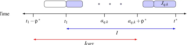
Proof. Recall that all requests inJI are completely satisfied duringI. Thus we have that the total size of requests inJI is|I|. By definition Jq,k witnesses a response time greater than 2ρ∗ and therefore
t∗−aq,k>2ρ∗. SinceJq,k∈JIis the last request done by FIFO duringI, all requests inJI must arrive no later thanaq,k. Therefore, these requests must be finished by timeaq,k+ρ∗by the optimal solution. From Lemma 3.3, all the requestsJI arrived no earlier thant1−ρ∗. Thus OPT must finish all requests inJI, whose total volume is|I|, duringIOPT= [t1−ρ∗,aq,k+ρ∗]. Thus it follows that|I| ≤ |[t1−ρ∗,aq,k+ρ∗]|, which simplifies tot∗≤aq,k+2ρ∗. This is a contradiction to the assumption thatt∗−aq,k>2ρ∗.
t1−ρ∗ t1 aq,k aq,k+ρ∗ t∗
Time
I
IOPT
Jq,k
Figure 1: Broadcasts by FIFO satisfying requests inJIare shown in blue. Note thataq,kandaq,k+ρ∗ are not necessarily contained inI.
3.2 Delay factor
In this section we consider minimizing the maximum delay factor in the broadcast setting. We start by showing that no 1-speed online algorithm can be(n/4)-competitive for minimizing the maximum delay factor wherenis the number of pages. We then prove the following theorem
Theorem 3.4. There is an online algorithm that is(1+ε)-speed O(1/ε2)-competitive for minimizing the
maximum weighted delay factor in the broadcast setting where pages have uniform size. For non-uniform sized pages there is a(1+ε)-speed O(1/ε3)-competitive online algorithm.
InSection 3.2.1we show a(1+ε)-speedO(1/ε2)-competitive online algorithm for uniform sized
pages and uniform weight requests. Finally, we extend our algorithm and analysis to the case of non-uniform page sizes and non-uniform weight requests to obtain a(1+ε)-speedO(1/ε3)-competitive online algorithm inSection 3.2.2. InSection 4we show how to extend these results to the case where requests have non-uniform weights.
Theorem 3.5. Every1-speed online deterministic algorithm for broadcast scheduling to minimize the maximum delay factor has a competitive ratio of at least n/4where n is the number of pages even when pages have uniform sizes.
Proof. The lower bound instance we construct is inspired by a lower bound given in [17]. LetAbe any online 1-speed algorithm and letnbe a multiple of 4. We consider the following adversary. At time 0, the adversary requests pages 1, . . . ,n/2, all which have a deadline ofn/2. Between time 1 andn/4 the adversary requests whatever page the online algorithmAbroadcasts immediately after that request is broadcast; this new request also has a deadline ofn/2. It follows that at timet=n/2 the online algorithm Ahasn/4 requests for distinct pages in its queue. However, the adversary can finish all these requests by timen/2. Then starting at timen/2 the adversary requestsn/2 new pages, say(n/2) +1, . . . ,n. These new pages are requested, one at each time step, in a cyclic fashion forn2 cycles. More formally, for i=1, . . . ,n/2, page(n/2) +iis requested at times j·(n/2) +i−1 for j=1, . . . ,n. Each of these requests has a slack of one which means that their deadline is one unit after their arrival. The adversary can satisfy these requests with delay since it has no queue at any time; thus its maximum delay factor is 1. However, the online algorithmAhasn/4 requests in its queue at timen/2; each of these has a slack ofn/2. We now argue that the delay factor ofAis at leastn/4. If the algorithm satisfies two slack 1 requests for the same page by a single transmission, then its delay factor isn/2; this follows since the requests for the same page aren/2 time units apart. Otherwise, the algorithm does not merge any requests for the same page and hence finishes the the last request by timen/2+n2/2+n/4. If the last request to be finished is a slack 1 request, then its delay factor is at leastn/4 since the last slack 1 requests is released at time n/2+n2/2. If the last request to be finished is one of the requests with slackn/2, then its delay factor is at least(n2/2)/(n/2) =n.
3.2.1 Uniform sized pages
algorithm that focuses on requests with the smallest slack can be made to do an arbitrary amount of “extra” work over the optimal schedule by repeatedly requesting the same page and giving the page small slack. The algorithm will repeatedly broadcast the same page while the adversary waits and satisfies multiple requests for this page with a single transmission. Further, we will show inSection 5that another greedy algorithm modeled after the well-studied algorithm Longest-Wait-First is not constant competitive with any fixed constant resource augmentation.
We begin by developing a variant of SSF thatadaptivelyintroduces a waiting time for requests. The algorithm uses a single real-valued parameterc<1 to control the waiting period. The algorithm SSF-W (SSF with waiting) is formally defined below. We note that the algorithm is non-preemptive in that a request once scheduled is not preempted. As we mentioned earlier, for uniform sized requests, preemption is not very helpful. At each time, the algorithm computes the delay factor of all requests in the algorithm’s queue, and considers requests for scheduling only when their delay factor is comparable to the request with maximum delay factor among the unsatisfied requests. Since our algorithm SSF schedules only the requests that have waited sufficiently long, the adversary cannot delay those requests to satisfy them with a less number of transmissions. We formalize this intuition inLemma 3.6.
Algorithm: SSF-W
• The algorithm is non-preemptive. Lett be a time that the machine is free (either because a request has just finished or there are no requests to process).
• LetQ(t)be the set of alive requests at timetand let
αt= max
Jp,i∈Q(t) max
1,t−ap,i
Sp,i
be the maximum current delay factor of requests inQ(t).
• Let
Q0(t) =nJp,i∈Q(t)
t−ap,i
Sp,i
≥ 1 cαt
o
be the set of requests inQ(t)with current delay factor at least 1cαt.
• Let Jp,i be the request in Q0(t) with the smallest slack. Broadcast page p non-preemptively.
We analyze SSF-W when it is given a(1+ε)-speed machine. Letc>1+2/εbe the constant which parameterizes SSF-W. Letσ be an arbitrary sequence of requests. We let OPT denote some fixed offline optimum schedule and letα∗andαSSF-W denote the maximum delay factor achieved by OPT
and SSF-W, respectively. We will show thatαSSF-W≤c2α∗. For the sake of contradiction, suppose that
(t1,t∗]if SSF-W is forced to broadcast by requestJp,iat timetit is the case that(t−ap,i)/Sp,i>α∗and
Sp,i≤Sq,k. We letI= [t1,t∗].2
We letJIdenote the requests which forced SSF-W to broadcast during the interval[t1,t∗]. We now show that any two requests inJI cannot be satisfied with a single broadcast by the optimal solution. Intuitively, the most effective way the adversary performs better than SSF-W is to merge requests of the same page into a single broadcast. Here we will show this is not possible for the requests inJI.
Lemma 3.6. OPTcannot merge any two requests inJI into a single broadcast.
Proof. LetJx,i,Jx,j∈JI such thati< j. Lett0 be the time that SSF-W starts satisfying requestJx,i. By the definition ofI, requestJx,i must have delay factor greater thanα∗at time fx,i. We also know that the requestJx,jmust arrive after timet0, otherwise requestJx,j must also be satisfied at timet0. If the optimal solution combines these requests into a single broadcast then the requestJx,imust wait until the request
Jx,jarrives to be satisfied. However, this means that the requestJx,imust achieve a delay factor greater thanα∗by OPT, a contradiction to the definition ofα∗.
To fully exploit the advantage of speed augmentation, we need to ensure that the length of the interval Iis sufficiently long.
Lemma 3.7. |I|=|[t1,t∗]| ≥(c2−c)Sq,kα∗.
Proof. The request Jq,k has delay factor greater thancα∗ at any time during I0 = [t0,t∗], where t0 =
t∗−(c2−c)Sq,kα∗. Letτ ∈I0. The largest delay factor any request can have at timeτis less thanc2α∗ by definition oft∗being the first time SSF-W witnesses delay factorc2α∗. Hence,ατ ≤c2α∗. Thus, the
requestJq,kis in the queueQ(τ)becausecα∗≥ατ/c. Moreover, this means that any request that forced
SSF-W to broadcast duringI0, must have delay factor greater thanα∗and sinceJq,k∈Q(τ)for anyτ∈I0, the requests scheduled duringI0must have slack at mostSq,k.
We now explain a high level view of how a contradiction is found. FromLemma 3.6, we know any two requests inJIcannot be merged by OPT. Thus if we show that OPT must finish all these requests during an interval which is not long enough to include all of them, we will have a contradiction. More precisely, we will show that all requests inJImust be finished duringIOPTby OPT, whereIOPT= [t1−2Sq,kα∗c,t∗]. It is easy to see that all these requests already have delay factorα∗by timet∗, thus the optimal solution
must finish them by timet∗. We first lower bound the arrival times of the requests inJI.
Lemma 3.8. Any request inJImust have arrived no earlier than t1−2Sq,kα∗c.
Proof. For the sake of contradiction, suppose that some requestJp,i∈JIarrived at timet0<t1−2Sq,kα∗c. Recall thatJp,ihas a slack no bigger thanSq,kby the definition ofI. Therefore at timet1−Sq,kα∗c,Jp,i has a delay factor greater thancα∗. Thus any request scheduled during the intervalI0= [t1−Sq,kα∗c,t1]
has a delay factor greater thanα∗. We observe thatJp,iis inQ(τ)forτ ∈I0; otherwise there must be a
request with a delay factor bigger thanc2α∗at timeτ and this is a contradiction to the assumption thatt∗
2The algorithm SSF-W was proposed in [23] and was shown to be(2+
ε)-speedO(1/ε2)-competitive. The improved
is the first time that SSF-W witnessed a delay factor ofc2α∗. Therefore any request scheduled duringI0
has a slack no bigger thanSp,i. Also we know thatSp,i≤Sq,k. In sum, we showed that any request done duringI0 had slack no bigger thanSq,k and a delay factor greater thanα∗, which is a contradiction to the
definition oft1.
Now we are ready to prove the competitiveness of SSF-W.
Lemma 3.9. Suppose c is a constant s.t. c>1+2/ε. If SSF-W has(1+ε)-speed thenαSSF-W≤c2α∗.
Proof. For the sake of contradiction, suppose thatαSSF-W>c2α∗. During the intervalI, the number of
broadcasts which SSF-W transmits is(1+ε)|I|. FromLemma 3.8, all the requests processed duringI have arrived no earlier thant1−2cα∗Sq,k. We know that the optimal solution must process these requests before timet∗because these requests have delay factor greater thanα∗byt∗. ByLemma 3.6the optimal
solution must make a unique broadcast for each of these requests. Thus, the optimal solution must finish all of these requests in 2cα∗Sq,k+|I|time steps. Thus, it must hold that(1+ε)|I| ≤2cα∗Sq,k+|I|. Using Lemma 3.7, this simplifies toc≤1+2/ε, which is a contradiction toc>1+2/ε.
The previous lemmas proves that SSF-W is a (1+ε)-speed O(1/ε2)-competitive algorithm for minimizing the maximum delay factor in broadcast scheduling with uniform sized pages whenc=1+3/ε.
3.2.2 Non-uniform sized pages
Here we extend our ideas to the case where pages can have non-uniform sizes for the objective of minimizing the maximum delay factor. For this problem, in [23] we developed a generalization of SSF-W and showed that it is a(4+ε)-speedO(1/ε2)-competitive algorithm. Later, we gave a(2+ε)-speed
O(1/ε2)-competitive algorithm using a similar proof technique as used in the uniform page size setting given in the paper [22]. In this paper we show a(1+ε)-speedO(1/ε3)-competitive online algorithm by improving our analyses based on the technique developed by Bansal, Krishnaswamy and Nagarajan [6] which considersfractionalschedules.
We elaborate on the model for non-uniform page sizes. Each pagephas size`p, which we assume for simplicity is an integer. Pagepconsists of uniform sized pieces(1,p),(2,p), . . .(`p,p). In a time slot one piece of a unique page can be broadcast by the server. A requestJp,iis satisfied if it receives each of the pieces of pagepinsequentialorder; in other words, we assume that the clients do not buffer the pieces if they are sent out of order. We assume preemption is allowed, and pieces of different pages can be interspersed. We call this model the integral broadcast setting. We now describe a relaxed notion of a schedule that we call a fractional schedule. In a fractional schedule the pieces of a page pare indistinguishable and the only relevant information are the time slots during whichpis transmitted. Now a requestJp,i is satisfied once`p pieces of page phave been broadcast. That is,Jp,i is satisfied once the server devotes`ptime slots to pagepafterap,i. A reduction in [6] gives a scheme that translates an algorithm with 1 speed for the fractional broadcast setting into a(1+ε0)-speed integer schedule where
the flow time, fi−ai, of each request increases by a factor of at most 8/ε0for any fixedε0>0. Using this technique, any schedule that iss-speedc-competitive for the fractional setting can be converted online into a schedule that iss(1+ε0)-speedO(c/ε0)-competitive for the integral setting. The algorithm used
requests for the page. The priority of a request is based on the flow time of the request in the fractional schedule; a smaller flow time corresponds to higher priority. Generally, the algorithm broadcasts the page with the highest priority unsatisfied request. We now restrict our attention to the fractional model.
We outline the details of modifications to SSF-W. As before, at any timet, the algorithm considers the alive requestsQ(t)and a subsetQ0(t) of requests that have waited sufficiently long; that is those with current delay factor at leastαt/cwhereαt is the maximum current delay factor for requests inQ(t). Among all requests inQ0(t)the algorithm picks the one with the smallest slack and broadcasts a unit amount of the page for that request; ties are broken arbitrarily. Recall that since the fractional setting is considered, the algorithm only needs to specify the page being broadcast and not the piece of the page. The algorithm may preempt the broadcast ofpthat is forced by requestJp,iif another requestJp0,j becomes available for scheduling such thatSp0,j <Sp,i. A key issue that differentiates the algorithms in [23,22] from the one here is that those algorithms directly generate an integral schedule; therefore they have to not only specify the page but also the piece of the page. In particular the algorithms in [23,22] could preempt the transmission of a pagepfor a requestJp,iand transmit pagain from the start if a new requestJp,i0 forparrives and has much smaller slack than that ofJp,i. In the sequential model this means that the work done forJp,i is “wasted” and it would be satisfied at the same time asJp,i0. In the fractional setting and the algorithm considered hereJp,iwould continue to be satisfied as ifJp,i0 did not arrive and prior transmission would not be wasted.
We now analyze the algorithm assuming that it has a(1+ε)-speed advantage over the optimal offline
algorithm. As before, letσ be an arbitrary sequence of requests. We let OPT denote some fixed offline
optimum schedule and letα∗denote the optimum delay factor. Let c>1+3/ε be the constant that parameterizes SSF-W. We will show thatαSSF-W≤c2α∗. For the sake of contradiction, suppose that
SSF-W witnesses a delay factor greater thanc2α∗. We consider thefirsttimet∗when SSF-W has some
request in its queue with delay factorc2α∗. Let the requestJq,k be a request which achieves the delay factorc2α∗at timet∗. Lett1be the smallest time less thant∗such that at each timetduring the interval (t1,t∗]if SSF-W is forced to broadcast by requestJp,iat timetit is the case that(t−ap,i)/Sp,i>α∗and
Sp,i≤Sq,k. Again, letI= [t1,t∗]. Notice that some requests that force SSF-W to broadcast duringI could
have started being satisfied beforet1. We now show a lemma analogous toLemma 3.6. We say that two
requests for the same pagepare satisfied simultaneously at timetif both requests are unsatisfied prior to t,pis broadcast at timet, and both requests receive`punits ofpafter their arrival.
Lemma 3.10. Consider any two distinct requests Jx,j and Jx,ifor some page x. If Jx,j forces SSF-W to
broadcast during I before ax,i, thenOPTcannot satisfy Jx,j and Jx,isimultaneously at any time.
Proof. Lett0be the time that SSF-W is forced to broadcast pagexbyJx,jwheret0<ax,i. By the definition ofI, requestJx,j must have delay factor greater thanα∗at timet0. Hence, if OPT satisfiesJx,iandJx,j simultaneously thenJx,j will have delay factor strictly larger thanα∗in OPT, a contradiction.
The following Lemmas3.11and3.12can be proved in the same way that Lemmas3.7and3.8are proved. This is because the algorithm SSF-W is designed to be oblivious to page sizes. Indeed, the key definitions in the proofs including the first timet∗that SSF-W witnesses delay factorc2α∗, the request
Lemma 3.11. |I|=|[t1,t∗]| ≥(c2−c)Sq,kα∗.
Lemma 3.12. Any request which forced SSF-W to schedule a page during I must have arrived after time t1−2Sq,kα∗c.
Using the previous lemmas we can bound the competitiveness of SSF-W.
Lemma 3.13. Suppose c is a constant s.t. c>1+2/ε. If SSF-W has(1+ε)-speed thenαSSF-W≤c2α∗.
Proof. For the sake of contradiction, suppose thatαSSF-W>c2α∗. During the intervalI, the number of
broadcasts which SSF-W transmits is(1+ε)|I|. FromLemma 3.12, all the requests that forced SSF-W to broadcast duringI have arrived no earlier thant1−2cα∗Sq,k. We know that the optimal solution must process these requests before timet∗ because these requests have delay factor greater thanα∗
byt∗. ByLemma 3.10the optimal solution cannot simultaneously satisfy two requestsJx,i and Jx,j that forced SSF-W to broadcast duringIifax,iis later than whenJx,iforced SSF-W to broadcast. This implies the optimal solution must broadcast at least(1+ε)|I|units in 2cα∗Sq,k+|I|time steps. Thus, it must hold that(1+ε)|I| ≤2cα∗Sq,k+|I|. UsingLemma 3.11, this simplifies toc≤1+2/ε, which is a contradiction toc>1+2/ε.
By settingc=1+3/ε we have the following theorem.
Theorem 3.14. The algorithm SSF-W is(1+ε)-speed O(1/ε2)-competitive for minimizing the maximum
delay factor in a fractional schedule when pages have non-uniform sizes.
Using the reduction of [6] previously discussed, we have shown the second part ofTheorem 3.4.
4
Weighted response time and weighed delay factor
We show the connection of our analysis of SSF and SSF-W to the problem of minimizing the maximum weightedresponse time. In the unicast setting for the problem of minimizing the maximum weighted response time, requests do not have deadlines, but have weights. Each requestJihas a positive weightwi. The goal is to minimize maxiwi(fi−ai). Similar to the algorithm SSF, we give the following algorithm called BWF (Biggest-Weight-First). The algorithm BWF always schedules the request with the largest weight.
Algorithm: BWF
• LetQ(t)be the set of alive requests att.
• LetJibe the request with the largest weight among requests inQ(t), ties broken by arrival time.
Similarly we can think of the problem of minimizing the maximum weighted delay factor. Here a requestJihas a deadlinediand a weightwi. The objective now is to minimize maxiwimax{1,(fi−ai)/Si}. Let the modified weight of a requestJi be defined asw0i=wi/Si. The algorithm BWF above when implemented with modified weights is the algorithm SRF (Smallest Ratio First). It is not difficult to adapt the analysis for SSF inSection 2to show that BWF is(1+ε)-speedO(1/ε)-competitive for the problem of minimizing the maximum weighted response time, and that SRF is(1+ε)-speedO(1/ε)-competitive
for the problem of minimizing the maximum weighted delay factor.
Now consider the problem of minimizing the maximum weighted response time in broadcast schedul-ing when pages have uniform sizes. A requestJp,ihas a weightwp,i. The goal is to minimize the maximum weighted response time maxp,iwp,i(fp,i−ap,i). We extend the algorithm BWF to get an algorithm called BWF-W for Biggest-Wait-First with Waiting. The algorithm is parameterized by a constantc>1. At any timetbefore broadcasting a page, BWF-W determines the largest weighted wait time of any request which has yet to be satisfied. Let this value beρt. The algorithm then chooses to broadcast a page corresponding to the request with largest weight amongst the requests whose current weighted wait time at timetis larger thanρt/c.
Algorithm: BWF-W
• The algorithm is non-preemptive. Lett be a time that the machine is free (either because a request has just finished or there are no requests to process).
• LetQ(t)be the set of alive requests at timetand letρt=maxJp,i∈Q(t)wp,i(t−ap,i).
• LetQ0(t) ={Jp,i∈Q(t)|wp,i(t−ap,i)≥1cρt}.
• Let Jp,i be the request in Q0(t) with the largest weight. Broadcast page p non-preemptively.
Although minimizing the maximum delay factor and minimizing the maximum weighted flow time are very similar metrics, the problems are not equivalent. It may also be of interest to minimize the maximumweighteddelay factor. In this setting each request has a deadline and a weight. The goal is to minimize maxp,iwp,imax{1,(fp,i−ap,i)/Sp,i}. For this setting we can simply alter BWF-W where we use modified weights for requests:w0p,ifor requestJp,iis defined aswp,i/Sp,i. We call the resulting algorithm SRF-W (Smallest-Ratio-First with Waiting).
For the problems of minimizing the maximum weighted response time and weighted delay factor, the upper bounds shown for SSF-W in this paper also hold for BWF and SRF-W, respectively. The analysis of BWF and SRF-W is very similar to that of SSF-W. To illustrate how the proofs extend, we prove that SRF-W is(1+ε)-speedO(1/ε2)-competitive for minimizing the maximum weighted delay factor
in broadcast scheduling where all pages are uniform sized and there is a single machine. This is the most general problem discussed as it is a generalization of weighted response time and the delay factor. We analyze SRF-W when it is given a(1+ε)-speed machine. Letc>1+2/ε be the constant which
parameterizes SRF-W. Letσ be an arbitrary sequence of requests. We let OPT denote some fixed offline
optimum schedule and letα∗andαSRF-Wdenote the maximum weighted delay factor achieved by OPT
SRF-W witnesses a weighted delay factor greater thanc2α∗. We consider thefirsttimet∗when SRF-W
has some request in its queue with weighted delay factorc2α∗. Let the requestJq,kbe a request which achieves the weighed delay factorc2α∗at timet∗. Lett1be the smallest time less thant∗such that at each
timetduring the interval(t1,t∗]if SRF-W is forced to broadcast by requestJp,iat timetit is the case that
wp,i(fp,i−ap,i)
Sp,i
>α∗ and Sp,i
wp,i
≤ Sq,k wq,k .
Throughout this section we letI= [t1,t∗].
We letJIdenote the requests which forced SRF-W to schedule broadcasts during the interval[t1,t∗].
We now show that any two request inJIcannot be satisfied with a single broadcast by the optimal solution.
Lemma 4.1. OPTcannot merge any two requests inJI into a single broadcast.
Proof. Let Jx,i,Jx,j ∈JI such that i< j. Lett0 be the time that SRF-W satisfies requestJx,i. By the definition ofI, requestJx,imust have weighted delay factor greater thanα∗at this time. We also know
that the requestJx,j must arrive after timet0, otherwise requestJx,j must also be satisfied at timet0. If the optimal solution combines these requests into a single broadcast then the requestJx,i must wait until the requestJx,j arrives to be satisfied. However, this means that the requestJx,imust achieve a weighted delay factor greater thanα∗by OPT, a contradiction.
As in the analysis of SSF-W we show that intervalIis sufficiently long.
Lemma 4.2. |I|=|[t1,t∗]| ≥(c2−c)Sq,k wq,kα
∗.
Proof. The requestJq,k has weighted delay factorcα∗at time
t0=t∗−(c2−c)Sq,k
wq,k α∗.
The largest weighted delay factor any request can have at timet0is less thanc2α∗by definition oft∗being the first time SRF-W witnesses weighted delay factorc2α∗. Hence,αt0≤c2α∗. Thus, the requestJq,kis in
Q(t0)becausecα∗≥αt0/c. Moreover, this means that any request that forced SRF-W to broadcast during
[t0,t∗], must have weighted delay factor greater thanα∗and sinceJq,k∈Q(t0), the requests scheduled during[t0,t∗]must have a ratio of slack over weight of at mostSq,k/wq,k.
Lemma 4.3. Any request inJImust have arrived after time t1−2 Sq,k wq,kα
∗c.
Proof. For the sake of contradiction, suppose that some requestJp,i∈JI arrived at time
t0<t1−2
Sq,k
wq,k α∗c.
Recall thatSp,i/wp,i≤Sq,k/wq,kby the definition ofI. Therefore at time
t1−
Sq,k
Jp,ihas a weighted delay factor greater thancα∗. Thus any request scheduled during the interval
I0=
t1−Sq,k wq,k
α∗c,t1
has a weighted delay factor greater thanα∗. We observe thatJp,iis inQ(τ)forτ∈I0; otherwise there must be a request with weighted delay factor bigger thanc2α∗at timeτ and this is a contradiction to
the assumption thatt∗is the first time that SRF-W witnessed a weighted delay factor ofc2α∗. Therefore
any request scheduled duringI0has a slack over weight no bigger thanSp,i/wp,i. Also we know that
Sp,i/wp,i≤Sq,k/wq,k. In sum, we showed that any request done duringI0 had slack over weight no bigger thanSq,k/wq,kand a delay factor greater thanα∗, which is a contradiction to the definition oft1.
Now we are ready to prove the competitiveness of SRF-W.
Lemma 4.4. Suppose c is a constant such that c>1+2/ε. If SRF-W has(1+ε)-speed thenαSRF-W≤
c2α∗.
Proof. For the sake of contradiction, suppose thatαSRF-W>c2α∗. During the intervalI, the number of broadcasts which SRF-W transmits is(1+ε)|I|. FromLemma 4.3, all the requests processed duringI
have arrived no earlier thant1−2cα∗Sq,k/wq,k. We know that the optimal solution must process these requests before timet∗ because these requests have weighted delay factor greater thanα∗ byt∗. By
Lemma 4.1the optimal solution must make a unique broadcast for each of these requests. Thus, the optimal solution must finish all of these requests in 2cα∗Sq,k/wq,k+|I|time steps. Thus it must hold that
(1+ε)|I| ≤2cα∗Sq,k
wq,k +|I|.
UsingLemma 4.2, this simplifies toc≤1+2/ε, which is a contradiction toc>1+2/ε.
5
Lower bound for a natural greedy algorithm LF
In this section, we consider a natural algorithm for minimizing the maximum delay factor which is similar to SSF-W. This algorithm, which we will call LF for Longest Delay First, always schedules the page which has the largest delay factor. We will consider the algorithm LF in the unicast scheduling setting when all requests have uniform sizes. Recall that the non-uniform requests setting can be reduced to the uniform request setting when preemption is permissible.
Algorithm: LF
• The algorithm is non-preemptive. Lettbe a time that the machine is free (either because a request has just finished or there are no requests to process).
• LetQ(t)be the set of alive requests att.
Notice that LF is the same as SSF-W whenc=1. However, we are able to show a negative result on this algorithm for minimizing the maximum delay factor. This demonstrates the importance of the trade-off between scheduling a request with smallest slack and scheduling the request with a large delay factor. The algorithm LF was suggested and analyzed in our work [21] and is inspired by LWF [21,29]. In [21] LF is shown to beO(k)-competitive withO(k)-speed forLknorms of flow time and delay factor in broadcast scheduling when pages have uniform sizes. It was suggested in [21] that LF may be competitive for minimizing the maximum delay factor (theL∞-norm). The rest of this section will be devoted to showing the following theorem.
Theorem 5.1. For any constant s>1, LF is not constant competitive with s-speed for minimizing the maximum delay factor (or weighted response time) in the unicast scheduling setting when requests have uniform sizes.
Since LF processes the requestJi such that(t−ai)/Siis maximized, it would be helpful to formally define the quantity. Let us define the wait ratio ofJi at timet≥ai as(t−ai)/Si; recall thatai andSi are the arrival time and slack size ofJi respectively. Note thatJi’s wait ratio at timeCi is the same as its delay factor ifJi has delay factor no smaller than 1. Further note thatJi’s delay factor is equal to max{1,(fi−ai)/Si}. The algorithm LF schedules the request with the largest wait ratio at each time. LF can be seen as a natural generalization of FIFO. This is because FIFO schedules the request with largest wait time at each time. Recall that SSF-W makes requests to wait to be scheduled to help merge potential requests in a single broadcast. The algorithm LF behaves similarly since it implicitly delays each request until it is the request with the largest wait ratio, potentially merging many requests into a single broadcast. Hence, this algorithm is a natural candidate for the problem of minimizing the maximum delay factor and it does not need any parameters as the algorithm SSF-W does. We show however that this algorithm does not have a constant competitive ratio with any constant speed.
We construct the following adversarial instanceσ for any integral speed-ups>1 and any integer c≥2; the assumption ofsandcbeing integral can be easily removed by multiplying the parameters in the instance by a sufficiently large constant. For this problem instance we will show that LF has wait ratio at leastc, while OPT has wait ratio at most 1. In the instanceσ there is a sequence of groups of
requests,Ji for 0≤i≤k, wherekis an integer to be fixed later. We now explain the requests in each group. For simplicity of notation and readability, we will allow requests to arrive at negative times. We can shift all of the arrival times later to make the arrival times positive. All requests have unit sizes. All requests in each groupJihave the same arrival time
Ai=−(sc)k−i+1− k−1−i
∑
j=0(sc)j
and have the same slack size
Si=
s(sc)k−i (1−1/sc)k−i.
For notational simplicity, we override the notationSito refer to the slack size of any request inJi, rather than to refer to the slack size of an individual requestJi. There ares(sc)k+1requests in groupJ0and
We now explain how LF and OPT behave for the instanceσ. Sometimes, we will useJi to refer to requests inJirather than explicitly saying “requests inJi,” since all requests in the same group are indistinguishable to the scheduler. For the first groupJ0, LF keeps processingJ0upon its arrival until
completing it. On the other hand, we let OPT procrastinateJ0until OPT finishes all requests inJ1toJk. This does not hurt OPT, since the slack size of the requests inJ0is large relative to other requests. For
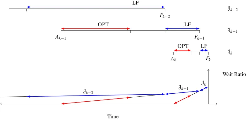
each groupJifor 1≤i≤k, OPT will startJiupon its arrival and complete each request inJiwithout interruption. To the contrary, for each 1≤i≤k, LF will not begin schedulingJiuntil finishing all requests inJi−1. In this way substantial delay is accumulated before LF processesJkand such a delay is critical for LF, since the slack ofJk is small. We refer the reader toFigure 2.
Ak Fk
OPT LF
Ak−1 Fk−1
OPT LF
Fk−2 LF
Wait Ratio
Jk Jk−1
Jk−2
Time
Jk Jk−1
Jk−2
Figure 2: Comparison of scheduling of groupJk,Jk−1, andJk−2by LF and OPT.
We now formally prove that LF has the maximum wait ratioc, while OPT has wait ratio at most 1 for the given problem instanceσ. Let
Fi=Ai+ (sc)k−i+1=− k−1−i
∑
j=0(sc)j, 0≤i≤k.
Letri(t)denote the wait ratio of any request inJiat timet. We fixkto be an integer such that
3sc
1− 1 sc
k c≤1.
Lemma 5.2. LF, given speed s, completely schedulesJ0during[A0,F0]andJiduring[Fi−1,Fi],1≤i≤k.
Further, the maximum wait ratio of any request inJkunder LF’s schedule is c.
Proof. Observe that the length of the time interval[A0,F0]is exactly the amount of time LF with speeds needs to completely processJ0, sinces|[A0,F0]|=s(sc)k+1=|J0|. Similarly we observe that the length of
First we show thatJ0 is finished during[A0,F0]by LF. Note that before timeF0, no request inJj,
j≥2 arrives, since
F0=− k−1
∑
j=0(sc)j≤ −(sc)k−1−
k−3
∑
j=0(sc)j=A2
and all requests inJj, j≥2 arrive no earlier than timeA2. We will show thatJ0has the same wait ratio
asJ1at timeF0. Then sinceJ0has a slack greater thanJ1, at any timetduring[A0,F0],r0(t)>r1(t)and
hence LF will work onJ0overJ1. Indeed, the wait ratio ofJ0at timeF0is
r0(F0) =
F0−A0
S0
= (sc) k+1
s(sc)k (1−1/sc)k
=c(1−1/sc)k,
which is equal to the wait ratio ofJ1at timeF0,
r1(F0) =F0−A1
S1 =
(sc)k−(sc)k−1 s(sc)k−1
(1−1/sc)k−1
=c(1−1/sc)k.
To complete the proof, we show thatJi,i≥1 is finished during[Fi−1,Fi]by LF. This proof is very similar to the above. Note that no request inJj, j≥i+2 arrives before timeFi, since
Fi=− k−1−i
∑
j=0(sc)j≤ −(sc)k−i−1−
k−3−i
∑
j=0(sc)j=Ai+2
and all requests inJj, j≤i+2 arrive no earlier than timeAi+2. We will show thatJihas the same wait ratio asJi+1at timeFi. Then since the slack ofJi+1is smaller thanJi, at any timetduring[Fi−1,Fi],Ji will have wait ratio no smaller thanJi+1and hence LF will work onJioverJi+1. Indeed, the wait ratio of
Jiat timeFi is
ri(Fi) =
Fi−Ai
Si
= (sc) k−i+1 s(sc)k−i (1−1/sc)k−i
=c(1−1/sc)k−i,
which is equal to the current delay factor ofJi+1at timeFi,
ri+1(Fi) =
Fi−Ai+1
Si+1
=(sc)
k−i−(sc)k−i−1 s(sc)k−1−i (1−1/sc)k−i−1
=c(1−1/sc)k−i.
Hence LF has wait ratio at leastcfor a certain request inJk.
In the following lemma, we show that there exists a feasible scheduling by OPT that has wait ratio at most 1, which together withLemma 5.2will complete the proof ofTheorem 5.1.
Lemma 5.3. Consider a schedule which processes all requests inJ0during[Fk,Fk+|J0|]and all requests
inJiduring[Ai,Ai+|Ji|]for1≤i≤k with speed1. This schedule is feasible and, moreover, the maximum
Proof. We first observe that the time intervals[Fk,Fk+|J0|]and[Ai,Ai+|Ji|]for 1≤i≤kdo not overlap, since fori≥1,
Ai+1−(Ai+|Ji|) = (sc)k+1−i+ (sc)k−1−i−s(sc)k−i−(sc)k−i≥(sc)k−i(sc−s−1)>0,
andFk−(Ak+|Jk|) =sc−s>0. Further, all requests inJ0can be completed during[Fk,Fk+|J0|]by a
scheduler with speed 1. Likewise, this shows that all requests inJican be completed during[Ai,Ai+|Ji|] by a scheduler with speed 1. Hence this is a feasible schedule for a 1 speed algorithm.
It now remains to upper bound the maximum wait ratio of any request under the suggested schedule. Consider any request inJi,i≥1. The maximum wait ratio ofJiunder the schedule is
Ai+|Ji| −Ai
Si
= s(sc) k−i s(sc)k−i (1−1/sc)k−i
= (1−1/sc)k−i<1.
The maximum wait ratio of any request inJ0is
r0(Fk+|J0|) =
Fk+|J0| −A0
S0 =
(s+1)(sc)k+1+∑kj−=01(sc) j
s(sc)k (1−1/sc)k
≤3s(sc)
k+1
s(sc)k (1−1/sc)k
=3sc(1−1/sc)k≤1.
The last inequality holds sincekwas chosen to satisfy the inequality.
6
Conclusions
We considered online scheduling to minimize maximum (weighted) response time and to minimize maximum (weighted) delay factor. Delay factor and the weighted response time metrics have not been previously considered. We developed scalable algorithms for these metrics in both the unicast and broadcast scheduling models. Our algorithms demonstrate an interesting trade off on whether to prioritize requests with larger weight or those that have waited longer in the system. Understanding this trade off has led to the first online scalable algorithm for minimizing average response time in broadcast scheduling [34] which has been an open problem for several years.
We close with the following open problems. Our algorithm for the maximum delay factor with uniform sized pages uses a parameter that explicitly depends on the speed given to the algorithm. Is there an algorithm that is scalable without needing this information? FIFO is 2-competitive for minimizing maximum response time in broadcast scheduling. In the offline setting can the 2-approximation implied by FIFO be improved? For the more general problem of minimizing maximum delay factor, no non-trivial offline approximation is known that does not use resource augmentation.