www.theoryofcomputing.org
Width-Parameterized SAT:
Time-Space Tradeoffs
Eric Allender
∗Shiteng Chen
†Tiancheng Lou
†Periklis A. Papakonstantinou
†Bangsheng Tang
†Received August 8, 2012; Revised July 14, 2013; Published October 8, 2014
Abstract: Alekhnovich and Razborov (2002) presented an algorithm that solves SAT on instancesφof sizenand tree-widthTW(φ), using time and space bounded by 2O(TW(φ))nO(1). Although several follow-up works appeared over the last decade, the first open question of Alekhnovich and Razborov remained essentially unresolved: Can one check satisfiability of formulas with small tree-width in polynomial space and time as above? We essentially resolve this question, by (1) giving a polynomial space algorithm with a slightly worse run-time, (2) providing a complexity-theoretic characterization of bounded tree-width SAT, which strongly suggests that no polynomial-space algorithm can run significantly faster, and (3) presenting a spectrum of algorithms trading off time for space, between ourPSPACE algorithm and the fastest known algorithm.
First, we give a simple algorithm that runs in polynomial space and achieves run-time 3TW(φ)lognnO(1), which approaches the run-time of Alekhnovich and Razborov (2002), but
∗Supported by National Science Foundation grants CCF-0832787 and CCF-1064785.
†Supported by National Basic Research Program of China Grant 2011CBA00300, 2011CBA00301, and the National Natural
Science Foundation of China Grant 61033001, 61061130540, 61073174, 61250110577.
ACM Classification:F.1.3, F.2.2
AMS Classification:68Q15, 68Q25
has an additional lognfactor in the exponent. Then, we conjecture that this annoying logn factor is in general unavoidable.
Our negative results show our conjecture true if one believes a well-known complexity assumption, which is theSC6=NCconjecture and its scaled variants. Technically, we base our result on the following lemma. For arbitraryk, SAT of tree-width logknis complete for the class of problems computed by circuits of logarithmic depth, semi-unbounded fan-in and size 2O(logkn)
(SAC1 whenk=1). Problems in this class can be solved simultaneously in time-space(2O(logk+1n),O(logk+1n)), and also in (2O(logkn), 2O(logkn)). Then, we show that our conjecture (for SAT instances with poly-log tree-width) is equivalent to the question of whether the small-space simulation of semi-unbounded circuit classes can be sped up without incurring a large space penalty. This is a recasting of the conjecture thatSAC1(and even its subclassNL) is not contained inSC.
Although we cannot hope for an improvement asymptotically in the exponent of time and space, we introduce a new algorithmic technique which trades constants in the exponents: for eachεwith 0<ε<1, we give an algorithm in time-space
31.441(1−ε)TW(φ)log|φ||φ|O(1),22εTW(φ)|
φ|O(1).
We systematically study the limitations of our technique for trading off time and space, and we show that our bounds are the best achievable using this technique.
1
Introduction
SAT is the prototypicalNP-complete problem. In the real-world SAT instances tend to have structure. Also, in practice SAT-solvers abort due to lack of memory. In this paper we provide conclusive, asymptotically tight answers regarding time-space tradeoffs for SAT instances that are structured, where this structure is quantified bytree-width.1
This restriction of SAT was studied by Alekhnovitch and Razborov [2] (for references prior to this see within), who gave algorithms that work in time 2O(TW(φ))|φ|O(1)and in space 2O(TW(φ))|φ|O(1), where
TW(φ)is the tree-width of a CNF formulaφ, and|φ|=n+mwherenandmare the number of variables and clauses, respectively. The authors of [2] state their results in terms of the branch-width of the formula, which is within a constant factor of the tree-width. They conclude:
“The first important problem is to overcome the main difficulty of the practical implementa-tion which is the huge amount of space used by width-based algorithms. . . . Thus we ask if one can do anything intelligent in polynomial space to check satisfiability of formulas with small branch-width?”
The question raised by Alekhnovich and Razborov is a major issue in practical SAT-solving. Modulo complexity assumptions we fully answer this question.
1.1 Our contribution and techniques
We devise a simple space-efficient algorithm for SAT instances in CNF, which runs in time
3TW(φ)log|φ||φ|O(1)
and space
|φ|O(1).
This is the first algorithm with running time exponential in the tree-width of the incidence graph (unlike [4] which is just on the primal graph) of arbitrary CNF instances (unlike [19] which is just fork-CNFs), that runs in polynomial space. Compared to the question of [2] this algorithm suffers a log|φ|factor in the exponent of the running time. Our work revolves around this logarithmic factor. First, we conjecture that it cannot be removed:
Conjecture 1.1. LetAbe an algorithm forSATthat runs in time2TW(φ)δ(|φ|)|φ|O(1). Consider CNF formulas whereTW(φ) =O(|φ|1−ε), for some fixed ε <1. If δ(φ) =o(log|φ|) then Auses space 2Ω(TW(φ)).
Second, we show that the above conjecture is equivalent to a widely-believed computational com-plexity assumption (scaled for a wider range of parameters). That is, we offer a comcom-plexity-theoretic connection that supports this conjecture. This computational complexity conjecture comes under the cryptic statementNC6⊆SC. This is well-known to complexity theorists, and also of immense practical interest.SCis the class of problems that can be decided by algorithms that work simultaneously in poly-logarithmic space and polynomial time (i. e., efficient time and efficient space computation).NCis the class of problems that can be decided by circuits simultaneously of polynomial size and poly-logarithmic depth (i. e., parallel computation which uses a small number of processors and small parallel time). There is an, almost exact, correspondence between algorithm space and circuit depth (e. g., given an algorithm that uses poly-logarithmic space we can construct a parallel algorithm that runs in poly-logarithmic parallel time) and between algorithm time and circuit size. These correspondences are believed to break down when wesimultaneouslybound “time and space” and simultaneously bound “size and depth.” That is,NC6⊆SCmeans that in general we cannot trade efficient #parallel processors-parallel time computation for efficient sequential time-space computation. Details and additional intuition are given inSection 3.
Semi-unbounded combinatorial circuits play an important role in this work. A semi-unbounded circuit (SAC) has AND gates of bounded fan-in, OR gates of unbounded fan-in, and all the negations at the input level. Despite their exotic nature these circuits have essential differences from bounded and unbounded fan-in circuits; seeSection 3.1for a discussion.
InSection 3we show:
Theorem 3.5.SAT of a given tree decomposition of width logknis complete for the class
SACkquasi:=SAC O(logn),2O(logkn),
i. e., semi-unbounded fan-in circuits ofO(logn)-depth, and 2O(logkn)-size.
whereNTISP denotes the set of problems decidable by non-deterministic Turing Machines that are simultaneously TIme-SPace bounded, and we show:
Theorem 3.6.SAT of a given path decomposition of width logknis complete forNSCk,
Note that the NSClevels are direct space-scaled analogs ofNLand theseSACclasses are direct size-scaled analogs ofSAC1. Therefore, separating the complexity of SAT parameterized by path-width and tree-path-width is equivalent to separating these classes, and hence, by padding, separatingNL andLOGCFL=SAC1. More importantly, putting these developments together we conclude that our conjecture impliesNC6=SC, and in fact as the tree-width ranges over different functions of the input length our conjecture is shown to be equivalent to a resource-scaled analog ofNC6=SC. Somewhat less rigorously:
Shrinking down the space, even by just a little, in a reasonably fast algorithm forSATof bounded tree-width, is the same as saying that every highly parallelizable problem can be sequentially computed simultaneously in small time and space.
Assuming for now thatConjecture 1.1holds, it makes sense to devise algorithms that approach these limits. This is the topic ofSection 4, which constitutes the more technically involved part of this work, though the practical significance of these algorithms is debatable.
We use our space-efficient algorithm, together with a time-efficient dynamic programming algorithm (essentially the algorithm of [35]), as the “end-points” for a spectrum of algorithms that trade off time and space complexity between these two extremes. But there is a catch. If we combine the time-efficient dynamic programming algorithm and our recursive algorithm in the obvious way, then we gain the worst of both worlds. Here “obvious” means that we discretize the space of truth assignments during the execution of the recursive algorithm and combine using dynamic programming. Instead, we introduce an implicit family of proof systems. We use two free parameters to specify an algorithm in this family. One parameter is an integer which is at least 2. This controls the “complexity” of the rules applied, for performing an unbalanced type of recursion of some sort. The larger this parameter is, the smaller the running time is and the more space is used. The second parameter is a real number in(0,1)that controls the discretization of the truth assignment space. This family of algorithms is presented inSection 4, and in its full generality inSection 5. In the same sections we show that all of the infinitely-many pairs of values are of interest, depending on the different time-space bounds one may want to achieve.
Remark 1.2. Throughout this paper we assume that the tree (or path) decompositions are given in the input. To the best of our knowledge, the same is true in all other works in width-parameterized SAT.
1.2 Related work
For SAT instances the tree-width of a CNF formula is the tree-width of its associated graph (e. g., incidence graph, primal graph, or intersection graph). Among those graphs, the most general one is the incidence graph (a bipartite graph where one side has variable-nodes and the other clause-nodes). In some sense, the tree-width value on the incidence graph lower bounds the tree-width value of the rest [37]. In particular, the tree-width of the incidence graph of a CNF formula can be arbitrarily smaller than the tree-width of the CNF-formula graphs that were studied by Bacchus et al. [4]. There is a vast literature (too large to concisely cite here) in empirical and theoretical studies in various width-parameterizations of SAT—we only cite some of the most relevant ones below.
Algorithms for width-parameterized SAT. Prior to our work, [4, 19] addressed the question of Alekhnovich and Razborov. In [19] the authors gave a combinatorially non-explicit algorithm only for thek-SAT problem, wherek is constant, where the algorithm runs in time 2O(TW(φ)log|φ|) and space |φ|O(1), whenTW(φ) =Ω(log|φ|). The deficiencies of [19] (which we overcome in our current paper) are not only that their algorithm works only fork-SAT, but also that the constant in the exponent of the running time cannot be bounded in any easy way due to the non-explicitness of the argument presented there. Bacchus et al. [4] present a polynomial-space DPLL algorithm with running time exponential in the tree-width of theprimal graphof a formula, hence their SAT algorithm is strictly weaker than ours (although they also present algorithms for #SAT and similar problems).
There have been a number of follow-ups improving the running time of the Alekhnovich and Razborov algorithm [2], considering different width-parameters: Fischer et al. [16] give algorithms for SAT (and a somewhat generalized version of #SAT) parameterized by tree-width and clique-width. Their tree-width algorithm matches the running time and space of an algorithm of Samer and Szeider [35], which we make use of later in this paper as a time-efficient algorithm, running in time-space
22TW(φ)|φ|O(1),2TW(φ)|φ|O(1).
Also, we remark that algorithms (e. g., for graph problems) which replace the tree-width parameter
TWin the exponent by aTW2 and at the same time reducing the space to polynomial (see e. g., [26]) are strictly worse than our algorithms (and in particular fail to reach our target lower bound for the Alekhnovitch-Razborov question). In particular, unlike the classical parameterized complexity approach, the interesting part of our treatment (and in particular our complexity results) are for values of tree-width that are related to the input length, and in factΩ(logn).
Finally, to the best of our knowledge our work is the first to address the issue of smooth time-space tradeoffs for width-parameterized SAT. Prior to our work there are others which solely discuss lower bounds on the running time; e. g., for graph problems (and under the very strong ETH assump-tion [22]) [25]. Another kind of tradeoff (between size of the separator and the sharpness) for graph problems was discussed in [17]. We should also mention that in two excellent works on constraint satisfaction problems Grohe [21] (assuming thatFPT6=W[1]) and Marx [27] (assuming ETH) essentially show that the running time of the known width-based algorithms is optimal.
Hardness results and complexity characterizations. Every problem inNPcan be seen as a problem where accepting instances can be verified in logarithmic space (i. e., we can settle for less than polynomial time in the verification). SAT of bounded path-width has been shown [30] complete for the class of problems that can be decided by a logarithmic space machine which has “streaming access” to the tape containing the witness; i. e., scanning the witness tape at most a given number of times. In particular, O(r(|φ|))passes correspond to SAT instances with given path-decompositions of widthr(|φ|)log|φ|. Specifically, deciding formulas with given path decompositions of widthO(log|φ|)is complete forNL, and [30] asks whether the complexity of SAT instances when the parameter is tree-widthO(log|φ|)is more difficult. In this paper we answer this question affirmatively, unless2 NL=SAC1. Furthermore, we show an exact correspondence of these “streaming verification” classes with the levels of the known NSChierarchy. Our new characterization through semi-unbounded circuits is of independent interest, and seems more natural than the characterizations presented in [1].
Relation to Propositional Proof Complexity. Our work opens new, exciting directions for Proposi-tional Proof Complexity. One way to make progress towards validatingConjecture 1.1 is to restrict attention to specific types of algorithms. The study of restricted proof systems is one such choice. In fact, Beame, Beck, and Impagliazzo [6] very recently made progress towardsexactlyvalidating our question. In particular, they proved a Resolution Refutation size-space tradeoff, which implies that there exists a family of formulasφ of tree-widthTW(φ)where for everyk>0 every resolution refutation of sizenk requires space
2TW(φ)log log loglog lognn.
This very significant development is the first super-polynomial lower bound of this sort, and through our work it can be interpreted as validating theSAC16⊆SCconjecture, at least for a class of restricted algorithms. This is a new direction; lower bounds in proof complexity are clearly connected to the NP6=coNPconjecture [15], but have not previously seemed to have a bearing on theSC6=NCquestion.
2
Preliminaries
We introduce notation, terminology, and conventions used throughout the paper.
2.1 Notation
All logarithms are of base 2, and all propositional formulas are in Conjunctive Normal Form (CNF). SAT is the decision problem where given an arbitrary CNF formula we want to decide if it is satisfiable. We letk-SAT denote the restriction of SAT to CNFs where each clause has at mostkliterals. For a formula φ,mdenotes the number of clauses,nthe number of variables, andCiandxjstand for thei-th clause and
j-th variable respectively. For convenience we write|φ|=m+n. When there is no confusion (e. g., when defining complexity classes)nis used to denote the input length.
2.2 Tree-width
Definition 2.1. Let G= (V,E) be an undirected graph. Atree decompositionofGis a tuple (T,X), whereT= (W,F)is a tree, andX={X1,· · ·,X|W|}whereXi⊆V such that
(1) S|W|
i=1Xi=V,
(2) ∀(i,j)∈E,∃t∈W, such thati,j∈Xt,
(3) ∀v, the set{t:v∈Xt}forms a subtree ofT.
Each ofXiis called abag, the width of(T,X)is defined as maxt∈W|Xt| −1, and thetree-widthTW(G)of
graphGis defined as the minimum width over all possible tree decompositions.
When the tree decompositionT= (W,F)is restricted to a path, the decomposition is called apath decomposition, and the specific tree-width is called the path-widthPW(G). The following inequality holds (e. g., [8])
TW(G)≤PW(G)≤O(log|V| ·TW(G)). (2.1) Definition 2.2. Theincidence graph Gφ of a SAT instanceφis a bipartite graph, where in one side of the bipartization each node is associated with a distinct variable, and in the other each node is associated with a clause. There is an edge between a clause-node and a variable-node if and only if the variable appears in a literal of the clause. The tree-width of a formulaφis the tree-width of its incidence graph,
TW(φ) =TW(Gφ).When it is clear from the context we may abuse notation and writeTW(φ)to denote
the width of a given decomposition of Gφ.
We assume that a tree decomposition of the incidence graph ofφ is given as input along withφ. For convenience, we assume without loss of generality that the input tree decompositions((W,F),X)have the following two properties.
(1) |W|=O(TW(φ)· |V|) =O(TW(φ)|φ|), and
(2) the treeT= (W,F)has bounded degree 3.
We call a tree decompositionniceif it satisfies the two properties above. A tree decomposition can be converted to a nice one in linear time (see e. g., [23,8]). The maximal degree in the tree decomposition is denoted byd. By the property above,d≤3. If the input is given with apathdecomposition, thend≤2.
2.3 Assignments
We introduce terminology and notation to talk about truth assignments on bags. LetX be a bag in the tree decomposition,Vbe the variables and Cbe the clauses inX. Also, nV=|V|andmC=|C|. An assignment RX for X is a binary vector of lengthnV+mC. The firstnV bits indicate the truth values
of the corresponding variables. Note that the term “assignment” does not correspond only to a “truth assignment” on the variables inX. It is an assignment of bit values both to variables and to clauses.
What values the lastmC bits have is a subtle issue explained inSection 4. For the dynamic program-ming algorithm things are pretty clear. However, for the space-efficient and trade-off algorithms, things become more subtle. Intuitively, a bit corresponding to a clauseCis 1 if we “have decided” to eventually satisfy this clause (this has to do with where we are in the execution of the algorithm). Such a decision is different for different algorithms, but we use the same data-structure.
Actually, the most straightforward way of defining the clause bits is to let it denote whether the corresponding clause “is” satisfied. To ensure that a clause is satisfied in one of the branches in the tree decomposition, we need to enumerate all 2d−1 combinations of branches on which the clause is satisfied. However, if one is interested in only the satisfiability problem (and not, e. g., in #SAT) we observe thatd combinations suffice.
3
A complexity-theoretic characterization
We show that (i) ourConjecture 1.1is equivalent to a widely believed complexity assumption (and its scaled analogs), and (ii) under a different well-known complexity assumption (NL(LOGCFL), for the same width parameterw(|φ|) SAT of tree-width O(w(|φ|))cannot be efficiently reduced to SAT of path-widthO(w(|φ|)). Both of these results follow by first proving that SAT parameterized by path-and tree-width is complete for natural complexity classes. To obtain these results, we heavily rely on properties of semi-unbounded combinatorial circuits. InSection 3.1we give a primer with basic intuition about these circuits. Also, based on properties of these circuits and on the relation between path-width and tree-width in equation (3.1) inSection 3.3, we provide a new characterization ofNSC.
3.1 A primer on semi-unbounded fan-in circuits
The statements of the lower bounds do not explicitly refer to semi-unbounded families of circuits, but we use them inside the arguments. A circuit is semi-unbounded when it has unbounded fan-in OR gates, bounded fan-inANDgates, and all the negations are at the input level. The class of problems that can be decided by such circuits of depthO(login)and polynomial size is denoted bySACi. Clearly, NCi⊆SACi⊆ACi, whereNCandACdenote the complexity classes characterized by the same parameters with bounded fan-in and unbounded fan-in families of circuits, respectively. There is also the issue of uniformity; we provide the necessary background regarding circuit uniformity in the next sub-section. For the moment, the reader should make use of an informal uniformity assumption, meaning merely that there is an efficient algorithm describing how to construct the circuits for inputs of sizen.
recursively thatC(x) =1. The standard algorithm would be to start at the output gate and execute the following recursive algorithm: if the current gategis an OR gate, nondeterministically pick a gateh that feeds intogand verify thathevaluates to 1; if the current gategis an AND gate withh1, . . . ,hm
feeding into it, recursively verify that each of thehievaluates to 1. An accepting run of this algorithm
corresponds to a (possibly huge) tree, called a “proof tree” [38]; if the circuitChas bounded fan-in (or even semi-unbounded fan-in), then the size of this tree is bounded by 2depth. In the bounded fan-in case, restricting the depth ofCautomatically implies restricting the size ofC; in the semi-unbounded fan-in case this is not true. The important aspect of semi-unbounded fan-in circuits that we will utilize, is that the proof tree can be much smaller than the circuit (unlike the bounded-fan-in case), and has size exponential in the depth (unlike the unbounded-fan-in case).
An observation on uniformity. Consider a family of semi-unbounded circuits of size 2nO(1) and depth O(logn)that is polynomial time uniform, in the sense that, given the names of two gatesgandh, one can determine in time polynomial innwhether there is an edge fromgtoh, and what kind of gatesgandh are. (Note thatnO(1)bits are required, merely to write down the name of one of the gates.) Then, for an inputx,|x|=n, the problem of evaluating the membership of the familyCn(x)is inNP. That is, given
xwe guess a proof as described above and then verify that it is a valid proof. Clearly, every problem L∈NPcan be computed by such a circuit since in logndepth we can verify that a given witnessyis an encoding of a valid accepting computation path on inputx, and hence we obtain a circuit forL∩ {0,1}n
by putting a bigORgate as the output gate, computing the disjunction, over all potential witnessesy, of theO(logn)depth circuit testing ifyis a witness for the inputx). In other words,NPis precisely the class of problems computed by uniform semi-unbounded circuits of size 2nO(1). Observe that if we do not insist on the uniformity, then an arbitrary function can be computed by a 2O(n)-size andO(logn)-depth semi-unbounded (non-uniform) circuit.
Relations of SAC circuits to other models of computation. Semi-unbounded fan-in circuits are intimately related to Alternating Turing Machines (ATMs) and to Nondeterministic Auxiliary PushDown Automata (NAuxPDAs). We provide definitions later on; for a more detailed treatment see, e. g., [34]. For the moment let us say that anATMand aNAuxPDAare basically the same thing. Also, recall that an ATMis a nondeterministic Turing Machine with two kinds of nondeterministic states: existential and universal. An existential state is accepting if and only if at least one successor configuration is accepting, whereas a universal state is accepting if and only if each successor configuration is accepting. Although it requires a bit of work to show equivalence [38] it should come at no surprise that proofs forSACcircuits are related toATMcomputations.
3.2 Complexity theory notation and some preliminaries
Conjecture 3.1. TheNL-complete graph reachability problem3cannot simultaneouslybe solved de-terministically in sub-polynomial space and polynomial time. That is, depth-first search cannot be simulated quickly in small space, and henceNL6⊆TISP(nO(1),no(1)). This implies the weaker conjecture SAC16⊆TISP(nO(1),no(1)).
We denote by SATtw(w(|φ|))the problem of deciding SAT of a given CNF formula together with a tree decomposition of widthw(|φ|). Similarly, for path-width we use the notation SATpw(w(|φ|)). [30] shows that SATpw(w(|φ|))is complete for the classNL[w(|φ|)/log|φ|], characterized by log-space bounded Turing Machines augmented with a polynomially long read-only, nondeterministic tape on which they makeO(w(|φ|)/log|φ|)passes.
We use the notationSAC(depth,size). We follow standard conventions when defining levels of theNC hierarchy, by definingSACk:=SAC(O(logkn),nO(1)). However, in this paper a different parameterization will be of equal importance: by restricting the depth of semi-unbounded fan-in circuits to beO(logn), and allowing the size to be quasipolynomial, we obtain subclasses ofNPdenoted by
SACkquasi:=SAC O(logn),2O(logkn).
The study ofSACcircuits, and the various classesSACihas received considerable attention, e. g., [12,38]. TheSACkquasi classes (very shallow quasi-polynomial size circuits) are introduced in this paper; they characterize the NSC hierarchy (equation (3.1)). For these families of circuits we use DLogTime -uniformity [5]. This means that thedirect connection languagefor the circuit family can be recognized in linear time. The direct connection language takes inputs of the formhn,i,d,j,tisuch thatd>0 and the dth input of the gateiin the circuit for inputs of lengthnis of typet(∈ {AND,OR,0,1})and has index j, or elsed=0 and gateiis of typet. Since the stringhn,i,d,j,tihas length logarithmic in the size of the circuit for inputs of lengthn, it follows that, forSACkquasicircuits, questions about connectivity in the circuits for lengthncan be answered in timeO(logkn).
Simultaneously depth-size bounded semi-unbounded circuits are intimately related to space-time boundedNAuxPDAs. ANAuxPDAis a nondeterministic space-bounded Turing Machine equipped with an unbounded stack (see [13] for a precise definition). NAuxPDA(s(n),t(n))is the class of languages decidable by aNAuxPDAin spaceO(s(n))and timeO(t(n)). Although general Turing machinetimeis related to circuitsizewhile circuitdepthis related tospace, onNAuxPDAs the correspondence is reversed; simultaneous bounds on circuit size and depth correspond to bounds on space and time, respectively. Generalizing the arguments in [34] and [38] we obtain:
Lemma 3.2. SACkquasi=NAuxPDA O(logkn),nO(1), for O(logkn)time uniformSACcircuits.
Proof. The proof ofSACkquasi⊇NAuxPDA(O(logkn),nO(1))can be shown by following the proof for the special casek=1 (i. e.,NAuxPDA(O(logn),nO(1)) =SAC(O(logn),nO(1))) [34,38]. (See also [39].) However, in the proof ofLemma 3.8we will need to assume that the uniformSACkquasi have certain properties, and thus we follow a different outline here, to establish that those properties hold.
Ruzzo [34, Theorem 1 & Corollary 7] showed that any language inNAuxPDA(O(logkn),nO(1))is accepted by aNAuxPDArespecting these same resource bounds, where additionally the height of the
pushdown isO(logk+1n) (and pushes and pops consist of moving strings of lengthO(logkn) to and from the stack—hence it is useful to think of the stack as having height logn, over “symbols” of length O(logkn)). It is easy to see that such a machine can also be assumed to be somewhat “oblivious,” in the sense that the positions of the worktape and input heads at timetare the same for all inputs of lengthn. Rossmanith and Niedermeier subsequently improved on this, to show that theNAuxPDAcan be assumed to be completely oblivious, in the sense that the sequences of pushes and pops are also the same for all inputs of lengthn[29, Theorem 28]. (Rossmanith and Niedermeier state their theorems in terms of machines with a logarithmic worktape bound, but their proof works also for larger space bounds, as long as the time is polynomial.) In particular, the pushes and pops follow a very regular pattern, so that the computation is divided into phases corresponding to the height of the stack. The computation starts and ends with stack height zero, and precisely half-way through the computation, the stack height is also zero. Call these three configurationsC0,D0, andE0. The computation fromC0 toD0and fromD0toE0all takes place with a stack height of at least 1 “symbol” (where the stack “symbols” are ofO(logkn)bits each); these are the two “phases” with height 1. In general, there are 2i phases with heighti, for each i≤imax=O(logn). Each such phase (fori<imax) has some start configurationCiand end configuration
Eithat take place at times that depend only on the input lengthn, and there is a configurationDithat also
has stack heighti, such that the computations betweenCiandDiand betweenDiandEihave exactly the
same length and are both phases with stack heighti+1. (The phases at heightimaxstart in a configuration Cthat has a number j≤nrecorded in it, and ends in a configuration that records the j-th input symbol; no stack manipulation occurs in such a phase.)
Thus in order to show that
NAuxPDA O(logkn),nO(1)⊆SACkquasi,
it suffices to build circuits to simulate oblivious machines that have this very restrictive computation pattern. The output gate will check if the height zero phase starts with the initial configurationC0and ends with the accepting configurationE0; it is anORgate, connected to gates labeled with triples(C0,D0,E0) for allD0, to see if there is a computation fromC0toE0passing throughD0. In general, gates labeled
(Ci,Di,Ei)(or(Ci,Di,Ei,γ)) whereCi,Di, andEiencode the worktape contents and input head positions
(but not the stack contents) for some phase with stack heighti(andγis a stack symbol of length logkn) areANDgates, testing whether there are computations fromCitoDiand fromDi toEi, respectively. The
children of theseANDgates, corresponding to some computation between stack heighticonfigurationsA andB, areORgates over all(Ci+1,Di+1,Ei+1,γ)such that:
• there is a move fromAtoCi+1pushingγ, and
• there is a move fromEi+1toBpoppingγ.
(Ifi+1=imax, then instead of(Ci+1,Di+1,Ei+1,γ), the gates have the format(Ci+1,Ei+1,γ), and these gates are (possibly negated) input gates, recording whether the given input symbol is consistent with a transition fromCi+1toEi+1.)
Now we prove the other direction:
NAuxPDA O(logkn),nO(1)⊇SAC O(logn),2O(logkn).
LetLhaveSAC(O(logn),2O(logkn))circuits. ANAuxPDAacceptsLas follows. On inputx, compute the name of the output gate of the circuit (call itg), and writegon the worktape. Start the routine EVAL(g), described below.
Algorithm 1EVAL(g)
1: ifgis a (negated) input gate connected to input bitxithen 2: accept iffxiis 1 (0, respectively)
3: end if
4: ifgis anORgatethen
5: nondeterministically guess a gate namehand check thath→gis an edge in the circuit
6: returnEVAL(h) 7: end if
8: ifgis anANDgatethen
9: compute the gatesh1andh2that feed intog
10: pushh2onto the stack and call EVAL(h1)
11: ifthis evaluates to 0then
12: halt and reject
13: else
14: returnEVAL(h2)
15: end if
16: end if
The run-time required to to evaluate a gategat depthdis 2dnO(1), assumingLOGSPACEuniformity. This is polynomial inn, sinced =O(logn). The space required is dominated by the number of bits needed, to write down the name of a gate, which isO(logkn).
This completes the proof, but let us mention here that later, inLemma 3.7andLemma 3.8, we show that SATtw(logk|φ|)is hard forSAC(O(logn),2log
kn
), and is contained in
NAuxPDA O(logkn),nO(1).
The reader may be surprised that acceptance of a super-polynomial size circuit can be verified in (nondeterministic) polynomial time. This is related to the structure and size ofproofsof accepting inputs for semi-unbounded circuits. In particular, the size of such a proof/certificate is exponential in the depth of the circuit (see the proof ofLemma 3.8for details).
3.3 Completeness forSATpw(logk|φ|)andSATtw(logk|φ|), and a new circuit
characteri-zation of theNSChierarchy
TW(G)logncan be shown via a reduction computable inLOGSPACE[10]. Putting these together (or this can also be seen via a direct argument) we have the following characterization of theNSClevels:
NL
|{z}
NSC1
⊆ SAC1
| {z }
SAC1 quasi
⊆NSC2⊆SAC2quasi⊆NSC3⊆ · · · ⊆NSC=SACquasi. (3.1)
Our completeness results require us to present upper bounds on the complexity of SAT with small tree-width and path-width. For these upper bounds, we need the notation ofconsistency. Since we have extended the notion of assignment to also include assignments toclauses, we also need to have a correspondingly extended notation of consistency of assignments. The rigorous definition of consistency is deferred until the next section; for this section it suffices to rely on an intuitive understanding of the notion. Intuitively, assignments to two bags are said to be consistent, if the bits corresponding to variables agree, and some additional constraints imposed by the bits corresponding to clauses are satisfied such that a satisfying truth assignment can be deduced. For this section, it suffices to know that, if assignments for two bags are written on the worktape, then it is very easy to determine if the assignments are consistent. Also, by the connectivity properties of tree decompositions, it suffices to check consistency of neighboring bags.
Now, we turn to showing these completeness results. The following lemma impliesTheorem 3.5.
Lemma 3.3. NSCk=NL[logk−1n], for k∈ Z+.
Proof. Let’s see whyNSCk⊆NL[logk−1n]first. LetMbe a machine that accepts a languageL∈NSCk. FromM, we construct a machineM0 that uses only logarithmic space on its worktape, and that makes O(logk−1n)passes over a tape of polynomial length that holds the sequence of “nondeterministic” bits. On accepting computations, the nondeterministic tape ofM0 will contain an encoding of a computation ofM: i. e., a sequence of encodings of successive configurations (from initial state to accepting state) of a complete run ofM accepting the given input. (Clearly, such an encoding will have polynomial length since the running time ofMis polynomial and the length of each configuration isO(logkn).) A configuration will include state, head position and worktape. Without loss of generality we assume that all the encodings of configurations have the same size, and that the worktape is divided evenly into blocks of lengthO(logn). Note that because of the locality of computation, two adjacent configurations only differ inO(1)bits; theith blocks of the worktape of two consecutive configurations will be identical when the head is not in the corresponding block, and otherwise will differ only inO(1)bits.
For the other direction, it is sufficient to present a complete problem forNL[logk−1n]that is contained inNSCk. SATpw(logk|φ|)is such a problem, by the following characterization:
Lemma 3.4([30]). SATpw(logk|φ|)is complete forNL[logk−1n], for k∈Z+, under log-space many-to-one reductions.
A nondeterministic machineM00for SATpw(logk|φ|)runs as follows: on its worktape,M00guesses assignments (each of length logk|φ|) for each bag, in the order of path decomposition (storing only the assignments for three bags at any one time). In order to check the correctness of the assignment for the jth bag, the assignments for bags j−1,j, and j+1 on the working tape, and the consistency of these assignments can be checked in polynomial time. By the properties of path decompositions, checking consistency of consecutive bags is sufficient for correctness.M00usesO(logkn)space and polynomial time.
Lemma 3.4andLemma 3.3immediately yield the following theorem:
Theorem 3.5. SATpw(logk|φ|)is complete forNSCk, for k∈Z+, under log-space many-to-one reduc-tions.
Theorem 3.6. SATtw(logk|φ|) is complete for SACkquasi, for k∈Z+, under log-space many-to-one reductions.
Proof. Containment is byLemma 3.7andLemma 3.2, and hardness is byLemma 3.8.
Lemma 3.7. SATtw(logk|φ|)∈NAuxPDA O(logkn),nO(1).
Proof. The algorithm witnessing this containment is very natural when expressed as aNAuxPDA; it is a modification of the algorithm in [19] with an additional trick to handle arbitrary CNF clauses, and has a very similar structure to the proof that SATpw(logk|φ|)is inNSCk.
TheNAuxPDAwill perform a depth-first traversal of the tree decomposition, guessing assignments corresponding to the bags (each of lengthO(logk|φ|)) using the worktape and the stack to check consis-tency of the assignments. More precisely, theNAuxPDAwill start at the root and guess an assignment for the root node, and then recursively search the tree rooted at that node, given the current assignment. To search the tree rooted at a given nodev, given an assignment, theNAuxPDAwill first check if vhas any children. If not, theNAuxPDA will halt and reject if the assignment is not accepting, and otherwise will pop the stack to continue searching the tree rooted atv’s parent. Otherwise, theNAuxPDA will guess assignments forv’s children (of which there are≤2), and check that the assignments are consistent, then push the second child and its assignment onto the stack, along with information aboutv and its assignment, and then search the tree rooted at the first child. When that subtree has been searched, theNAuxPDAwill pop the information for the second child off of the stack and search it. If both subtrees are successfully searched, then theNAuxPDApops the stack to continue searching the tree rooted atv’s parent.
Hardness is more interesting. We do a reduction from an arbitrary language inSACkquasi. Similar “generic reductions” (i. e., reducing the computation of families ofSACcircuits) for tree-width-related
problems have appeared before, e. g., [20] .
Lemma 3.8. SATtw(logk|φ|)is hard forSACkquasi, underLOGSPACEmany-to-one reductions.
Proof. FixL∈SACk
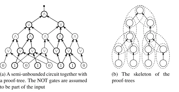
quasi and an inputx. LetCbe the associatedSACcircuit, with uniformity realized by a Turing MachineM(i. e., the machine that decides the direct connection language). We construct a formulaφthat is satisfiable if and only ifC(x) =1. Without loss of generality we assume the that the circuitCis of the type constructed in the proof of the first part ofLemma 3.2. In particular, note that we may assume the following normal form forC: (i)Cislayered, (ii)Cisstrictly alternating: odd-layer gates areOR, even-layer gates areAND, (iii)Chas an odd number of layers, and (iv) theANDgates inC have fan-in 2.
(a) A semi-unbounded circuit together with a proof-tree. The NOT gates are assumed to be part of the input
(b) The skeleton of the proof-trees
Figure 1: Proof-tree. In (b), a SATtw(logk|φ|)instance is constructed from the skeleton: each node corresponds toO(logkn)Boolean variables; clauses are constructed for each oval with dashed border; and only those variables corresponding to a node shared by different dashed circles must be put into a bag in the tree decomposition. This ensuresO(logkn)tree-width.
Aproof-treeis a tree with the same layering as the circuit. Each node of the tree is labelled by an index of a gate from the corresponding layer of the circuit. At odd layers, each node has one child, while at even layers, each node has two children. Two connected nodes must be labelled such that the corresponding gates are connected. At the bottom layer, each node must be labelled by an input gate or a NOT gate which outputs value 1. SeeFigure 1afor an illustration of an example.
aNAuxPDAwith thesamestart and end times. We encode this labeling as a CNF formula as follows. Associate a nodevin the skeleton with bit vectorsxv,dv,tv, where|xv|=|dv|=logkn,|tv|is constant. An
assignment to these Boolean vectors can be viewed as a labeling in the following sense:xvindicates the
index of the gate,tvindicates its type, whiledvtogether with anotherxuindicates which predecessor in the
circuit it should choose in the proof-tree. More specifically, for every nodevat an even-numbered layer in the skeleton with childrenul,urwe have: M(hn,xv,0,0,ANDi) =1,M(hn,xv,dv,xul,ORi) =1,and M(hn,xv,dv,xur,ORi) =1.Whenvis at an odd-layer, anduis its child, we haveM(hn,xv,0,0,ORi) =1, and eitherM(hn,xv,dv,xu,ANDi) =1 orM(hn,xv,dv,xu,1i) =1.
A correct proof-tree exists if and only if, for each edge(v,u), in the skeleton, the assignments to the variables inxv,dvandxucan be picked so thatMaccepts the corresponding tuples. This condition
can be formalized as∃s,M0(s) =1, where|s|=O(logkn), corresponding to the input bits provided to a Turing machineM0(a modification ofM) having running timeO(logkn)ons. We would like to encode this à la Cook-Levin (see e. g., [3]) as a CNF of sizeO(logkn)—but there is a catch. Using the tools provided in [3], this is only possible ifM0 isoblivious—and a naïve approach to makingM0 oblivious would introduce an unwanted log lognfactor; thus we need to look more closely at the condition thatM0 is checking.
M0 is takingsas input, and checking thatsis giving information about adjacent gates inC. Since all of the valid labels for a node in the skeleton are concerned with thesamesegment of an oblivious NAuxPDA’s computation, we can use the standard technique (e. g., [3]) to build a CNF of sizeO(logkn)
verifying that the connectivity information is correct. (For example,scould give the encodings for gates labeled(A,B)and(C,D,E,γ), and we need to verify that theNAuxPDAcan move fromAtoCpushing γ, and move fromE toBpoppingγ). At the end we take the conjunction of all the CNFs corresponding to the nodes and edges, which is also a CNFF, whereF is satisfiable if and only ifC(x) =1.
It remains to show thatF has tree-widthO(logkn). Notice that clauses inF are defined for only one specific node, and variables appear in clauses corresponding to at most two nodes. Therefore there is a natural tree decomposition associated withF, as illustrated inFigure 1b, that is, clauses and variables corresponding to an edge in the skeleton form a bag, and two bags are connected when they share variables. By the argument above, this tree decomposition has tree-widthO(logkn).
Remark 3.9. In general, when the tree-width is anything larger than poly-logarithmic, the previous reductions still hold. In particular, SATtw(w(|φ|))is complete for
SAC O(log|φ|),2O(w(|φ|)).
Remark 3.10. The proof ofLemma 3.8constructs a SAT instanceφ for which not only theincidence graph has small treewidth, but also theprimal graphhas small treewidth. Thus, although the treewidth of the primal graph can bemuchlarger than the treewidth of the incidence graph, SAT instances of small treewidth are complete for theSACkquasiclasses, no matter whether treewidth is measured with respect to the incidence graph, as in this paper, or with respect to the primal graph, as in [4].
3.4 ConnectingConjecture 1.1to complexity theory assumptions and the separation of
SATpw(logk|φ|)fromSATtw(logk|φ|)
Corollary 3.11. SACkquasi6⊆TISP 2O(logkn)
,no(1) ⇐⇒ Conjecture 1.1for tree-width O(logk|φ|).
In particular, whenk=1, we have thatConjecture 1.1for tree-widthO(log|φ|)is equivalent to
SAC16⊆TISP nO(1),no(1).
This corollary is just a resource-scaled form of our initial equivalence for logarithmic tree-width. In fact, by padding4we have:
Corollary 3.12. Conjecture 1.1for tree-widthpolylog(|φ|) =⇒ SAC16⊆SC.
Thus, modulo these complexity assumptions this settles the lower bound of the Alekhnovich-Razborov question. Note thatCorollary 3.12opens new avenues for propositional proof complexity [6]; i. e., validating our conjecture for restricted types of algorithms implies progress towardsNC6=SC.
As another corollary, assuming thatNL(SAC1, we separate the complexity of SAT
pwand SATtw.
Corollary 3.13. SATtw(log|φ|)is not log-space reducible toSATpw(log|φ|), unlessNL=SAC1.
In fact, the above holds up to NL-reductions. This corollary extends to every poly-logarithmic width under the scaled assumptionNSCk (SACkquasi. This is the first separation result for width pa-rameterizations of SAT for the same width parameter. Prior to our work there were only results in the opposite direction [19], where some width parameters (e. g., band-width and path-width) were shown to be log-space-equivalent, although combinatorially they can be off by an exponential.
4
Tradeoff algorithms on a single parameter
We consider two basic algorithms. One is time-efficient, which works in time-space
22TW(φ)|φ|O(1),2TW(φ)|φ|O(1),
whereas the space-efficient one works in time-space
3TW(φ)log|φ||φ|O(1),|φ|O(1).
The first one [35] is the most time-efficient (with respect to the constant in the exponent) algorithm known. The second is our contribution, and it is the first space-efficient algorithm for arbitrary CNFs for tree decompositions on the incidence graph. Our main contribution is combining these two algorithms in a non-trivial way to obtain a tradeoff. Later on, inSection 4.1, we provide a primer to algorithms for SAT instances with given tree decompositions.
4Philosophically, the assumption
SACkquasi6⊆TISP 2O(logkn),no(1)
Overview of the time- and space- efficient algorithms. The time-efficient algorithm does dynamic programming using the tree decomposition in a typical way [7]: root the tree to make it a binary tree, then for each bag define a 2TW(φ)size Boolean array; entry jin the array will be 1 if the subformula rooted at the bag is satisfiable, when the variables are given assignment j, and will be 0 otherwise. Clearly, computing the array for the root will solve the satisfiability of the formula, and indeed by the property of a tree decomposition, the array values can be computed in a leaves-to-root fashion.
To simplify the overview of the space-efficient algorithm we shall temporarily assume that each clause appears in a bag together with all of its variables.5 Observe that if we fix a truth assignment on a bag, then solving SAT on the given tree decomposition reduces to solving e. g., 3 independent subproblems—think of splitting the degree-3 tree into three subtrees by cutting the original one at this bag. The algorithm works by recursively enumerating and checking truth assignments on the bags. Its performance is determined by the size of the subproblems (ideally all the subtrees have the same size). In
Section 4.2(Lemma 4.2below) we show that there always exists a good choice for a bag, reminiscent to the well-known “1⁄3-2⁄3lemma” for binary trees. The lemmas inSection 4.2are a bit of an overkill for the
analysis of this simple algorithm, but they are also applied in the analysis of the tradeoff.
The tradeoff algorithm: where is the complication? Let us consider for a moment an execution of the space-bounded algorithm. We can visualize each step of the recursion as splitting the tree decomposition at a node (bag)—this bag is replicated at each of the subproblems with the fixed truth assignment. Let the process evolve for a while, and when the forest has enough trees let us single out one such tree. At the boundary (the leaves) of this tree there can be as many as log|φ|nodes to which we previously fixed an assignment, i. e., by splitting. The logarithmically large number of nodes does not affect the performance of the space-efficient algorithm(at each point of the recursion each bag/node is associated with a single assignment). Now, we switch gears to devise a tradeoff algorithm. A natural thing to do is first to discretize the truth assignment space associated with each bag, say in 2(1−ε)TW(φ)many chunks each of size 2εTW(φ), and we perform the recursion as in the space-efficient algorithm but now instead of
one assignment we assign the whole chunk. This brings the enumeration, at each recursive step, from 2TW(φ)down to 2(1−ε)TW(φ). On the other hand combining the chunks of the truth assignments into one consistent chunk associated with this tree may increase the space as much as 2εlog|φ|TW(φ). Overall this is
a time-space
2(1−ε)log|φ|TW(φ),2εlog|φ|TW(φ)
algorithm, worse both than the time- and space-efficient ones! To devise our tradeoff algorithm we show that it is possible tosimultaneously(i) perform the splitting in a way that at each step of the execution the forest consists of trees each with at most a constant number of split-nodes and (ii) this splitting results in subproblems of somewhat balanced sizes. Furthermore, we show that it is possible to control the number of splitting nodes per tree in the forest in a way that yields a tradeoff on this parameter (Section 5). This is a different (and competing) tradeoff from the one by the discretization factorε; i. e., our most general tradeoff algorithm is controlled by two parameters.
4.1 A primer to algorithms for width-parameterizedSAT
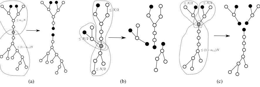
The structure of a tree decomposition is associated with the concept of separability (see e. g., [8]). Intuitively, the smaller the tree-width is, the easier the graph can be broken into separate components by removing nodes. Separability allows us to devise more efficient algorithms for small tree-width SAT than for general SAT. In some sense, the given tree decomposition allows us to “localize” an exhaustive search. The following example sheds some light on how this can be done towards devising a space-bounded algorithm. Recall that, for this initial overview, we are assuming that all the variables of a clause appear in the same bag with the clauses. We will see later that removing this assumption in a time-efficient manner is non-trivial (in fact, removing it without increasing the base of the exponential running time is an interesting puzzle).
(a) Input tree decomposition.
+
(b) Fixing an assignment to the variables in the middle bag results in two indepen-dent instances.
Figure 2: An example showing bounded tree-width SAT can be solved efficiently.
Supposexi’s,x0i’s andxi00’s are different sets of variables and the tree decomposition is as inFigure 2a.
Let us fix a truth assignment to the variables in the bag in the middle, e. g.,x1=x2=x3=x4=1. Conditioned on this truth assignment we can simplify the instance by removing clauses that are already satisfied, and removing literals in a clause that are set to false. This will result in multiple sub-instances as shown inFigure 2b. The properties of a tree decomposition assure that the sub-instances depend on different sets of variables, i. e., they areindependent. Since if instead they shared a common variable, this variable would have appeared in the middle bag, e. g.,x2. But this variable is already fixed by the truth assignment.
The satisfiability of the input instance, conditioned on the truth assignment given to the middle bag, is determined by the satisfiability of the two separate sub-instances. Therefore, it suffices to enumerate all truth assignments satisfying all the clauses in the middle bag without causing empty clauses in the simplification phase. Then, recurse into the two independent sub-instances to decide the satisfiability of the original instance. Furthermore, by choosing the middle bag carefully we can invoke this “splitting” on subtrees of somewhat balanced size.
all the clauses in the chosen bag, which costs O(2TW(φ)|φ|O(1)) time, and the total running time is O(2TW(φ)log|φ||φ|O(1)), which is much better than the current best algorithms for general SAT, which run in time exponential in|φ|.
The subtle additional assumption. The assumption that all variables of a clause appear in the same bag with the clause is not a mild one (especially for CNFs of large cardinality). Of course, in the actual algorithms we make no such assumption. In general, we may have to delay the decision to satisfy a clause. In the above algorithm, we only store the truth assignments to the variables. The following example shows that only storing this information is not enough when aiming at removing the assumption.
(a)φ1 (b)φ3
(c)φ2
Figure 3: Three instances used in the example. Figures on the top are the input tree decompositions, the bottom figures are the two components after fixing assignment to the variables in the middle bag.
SupposeC1=x1∨x2∨x4∨x6,C2=x1∨x3∨x5,C3=x2,C4=x3,C5=x4,C6=x5andC7=x6. Three instancesφ1,φ2andφ3along with their tree decompositions are given inFigure 3, whereφ1=C1∧· · ·∧C7, φ2=C1∧ · · · ∧C5∧C7(i. e.,C6is missing), andφ3=C1∧ · · · ∧C4∧C6∧C7(i. e.,C5is missing). We say that a clause is satisfied by a literal under a truth assignment if the literal appears in the clause and is set to 1. If an instance is satisfiable, then there is a truth assignment where every clause is satisfied by one of its literals.
Now, consider the splitting operation on the middle bag by fixing a truth assignment to it as above. For all three instances, the only possible assignment forx6 is 0, sinceC7must be satisfied byx6=0. Similarly, in the left bag, we must assignx2=0 andx3=0 to satisfyC3andC4. In the left bag, the only variable left isx1, which can satisfy eitherC1orC2but not both. The three instances differ in the right part where two variablesx4andx5are left.
is already satisfied, whileφ3is satisfied only whenC2is already satisfied. This piece of information is not carried through the middle bag by just the truth assignment to the variables. To overcome this issue we are going to use “clause-bits,” which we mentioned briefly inSection 2.3.
4.2 Splitting, consistency, assignment groups
In this section we give some additional notation and technical lemmas which we apply in the analysis of the space-efficient (Section 4.3) and tradeoff algorithms (Sections 4.4and 5). First we define an operation which allows a natural divide-and-conquer strategy, and a lemma follows the definition for choosing where the operation should occur. Then we define consistency with respect to our definition of assignments, which is somehow subtle and different from consistency of truth assignments. And in the last part of this section, we define a type ofdiscretized assignmentwhich is crucial in the tradeoff algorithms.
Definition 4.1(Splitting operation). LetT= (V,E)be a tree, andv∈V.Splitting T at vis the following operation. LetT1, . . . ,Tk be the trees after removingvfromT. The splitting operation results in a forest
{v} ∪T1, . . . ,{v} ∪Tk, where{v} ∪Ti is the subtree induced by the nodes inTitogether withv.vis called
thesplitting nodeof this operation.
Given a treeTtogether with a sequence of splitting operations results in a forest where each subtree in the forest in general has many nodes marked as splitting nodes. Splitting nodes before a specific splitting operation are calledprevious splitting nodes. A splitting operation also splits the set of previous splitting nodesSintoSi’s, whereSi is the set of splitting nodes contained in treeTi, 1≤i≤k.
Note that a splitting operation on a tree will result in a forest with more nodes than before, since we duplicate the splitting node and let it appear in each resulting tree. This fact will complicate the analysis of a recursive procedure. To overcome this, consider for each node, we created−1 replicas. When a splitting operation occurs, each replica of the splitting node goes to one of the branches (and redundant ones get removed if there are). Each node can be treated as splitting node only once, so the replicas of a node will be distributed only once. These slightly modified splitting operations will never increase the number of nodes. When analyzing running time on a tree originally withNnodes, one needs to used·N as a upper bound of the number of nodes. We will see that this is negligible since the number of nodes only appears as a polynomial factor or an argument logarithmically in the exponent of the running time. For ease of exposure, we will stick to the notationN as the number of nodes, while this should be the number after replicating.
Asplitting algorithmAcomputes a function that, given a treeTtogether with previous splitting nodesS, returns a node where the next splitting operation is going to be performed. A splitting algorithm formalizes the way of breaking an instance into sub-instances in the space-efficient algorithm. In particular, choosing thebalancing splitting nodeis done according to the following lemma.
Proof. We prove this lemma by giving an algorithm for finding p. First root the given tree at s, and then we iteratively construct a pathhs≡v1,v2, . . . ,v`ias follows. After constructing the path fromv1 throughvi−1,vi is chosen to be child ofvi−1which roots the largest subtree. We claim that there exists an α-splitting node in this path.
Denote byaithe size of the subtree containingsafter splitting atvi, 1≤i≤`. It is not hard to see that
a1=1,a`=N, andaistrictly increases asiincreases. Therefore, there must be a j, such thataj≤αN andaj+1>αN. We claim thatvj is the node we need. Ifaj+1−aj=1, then splitting atvj results in
two components, where the size of the component containingsisdαNe, while the other one is of size d(1−α)Ne. Ifaj+1−aj>1, then there must be a branch atvj, meaning thatvjhas at least two children.
Splitting atvjresults in at least three components. One which containssand is of size smaller thanαN.
The largest one among the rest is of size smaller than(1−α)N.
Corollary 4.3. On a bounded-degree tree of size N, there exists a node p, such that after splitting at p each subtree is of size at mostdN/2e.
Consistent assignments. In what follows we assume that there is an initial tree decomposition (recall that the bags are denoted byXi) together with a sequence of splitting operationsSthat results in the
subtrees along with their splitting nodes.
We refer to anassignment on a subtreeas the assignment that corresponds only to its splitting nodes. Formally, letX∗=S
vi∈SXi, and letVbe the variables andCthe clauses which have corresponding nodes inX∗. X∗ is the set of variables and clauses on which we define assignments. Suppose in one single splitting operation at the nodep, to whichXpis the corresponding bag,Tsplits into subtreesTi’s. Further
supposeRTis an assignment toT, andRTi is an assignment to the subtreeTi. Note that the only difference
betweenRTandRTi’s is atXp, andRT andRTi’s are said to beconsistentif
(1) for a variablex:
a) ifxappears inXp, then all the bits forxin eachRTi are assigned to the same value;
b) otherwise, all the bits forxare assigned to the same value as inRT;
(2) for a clauseC:
a) ifCappears inX∗and is assigned to 0, then∀ievery bit forCinRTi is assigned to 0;
b) otherwise,∃exactly oneisuch that inRTi the bit corresponding toCis assigned to 1.
Remark 4.4. The latter point in the definition, where in exactly one of the subtrees we require that the corresponding bit equals to 1, is somewhat subtle. The following lemma crucially depends on this property.
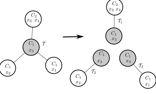
Lemma 4.5. For every assignmentRT to the treeT, the number of assignments RTi to subtreesTi’s
Figure 4: Consistent assignments. C1=x1∨x2∨x3,C2=x3∨x4. Consider splitting at the gray bag, while fixing the value of the bits, 1 forC1, 0 forx3. Any possible consistent assignments forT1,T2,T3 will have 0 forx3; in this consistent assignmentC1has value 1 inT1, and has value 0 inT2andT3.
Proof. LetXpbe the bag corresponding to the splitting nodep. For each variablexin the bagXp, there
are 2 possible assignments of the bit forxin theTi’s. For each clauseCinXp, ifCappears inRT and is
assigned to 0, by the definition of consistency, all the bits forCin theTi’s are assigned to 0. Otherwise,
in exactly oneTi, the bit forCis assigned to 1; in this case there are at mostdvalid assignments. Recall
thatdis the maximum degree of the tree decomposition.
We define a satisfying assignment in a way consistent with the role of clause bits in the assignments.
Definition 4.6. For a treeTwith splitting nodesS, an assignmentRTissatisfyingif there exists a truth assignmentAto every variable inT, such that
(1) every truth value for a variable inRT agrees with the corresponding value inA,
(2) every clauseCthat appears inTwhereCdoes not appear inS, is satisfied byA,
(3) every clauseCthat appears inSand the corresponding bit is assigned to 1 byRTis satisfied byA.
A satisfying assignment of the input tree decomposition with empty splitting nodeset implies that the input formula is satisfiable. The following lemma shows that the task of finding a satisfying assignment can be done recursively.
Lemma 4.7. An assignment RTissatisfyingif and only if there exist asatisfyingassignment RTi to each subtreeTi, such that all of the assignments RTi are consistent with RT.
Proof. For a treeTwith splitting nodesS, suppose that splitting at node presults in the subtrees{Ti}.
consistent withRT, such that for these truth assignments the conditions inDefinition 4.6are met. (Some of the clause bits in theRTi may need to be set to zero, to ensure consistency.)
For the other direction suppose that there exist assignmentsRTi of the subtreesTi, such that the
assignmentsRTi’s are consistent withRTand allRTi’s aresatisfying. For each subtreeTi, there exists a
truth assignment complying toDefinition 4.6. Since all these truth assignments agree on their common variables (because the common variables appear in splitting nodes inS), we can get a truth assignment from their union, which also meets the axioms in Definition 4.6. Therefore, the assignment RT is satisfying.
Anε-assignment groupε-GRTis a set of all possible assignments toS, where at most(1−ε)|S|TW(φ) entries are fixed. By definition,ε-assignment groups can be identified by the fixed entries. Consider a treeT,ε-assignment groupε-GRT, and subtreesTiresulting from a split at some node p. Consider one
such subtreeTi; letSibe the set of splitting nodes forTi, and note thatSi⊆S∪ {p}(and very likely it is a
proper subset). By fixing the “first”(1−ε)TW(φ)entries corresponding to variables or clauses contained in the nodep∈Si(using some fixed ordering), one obtains anε-assignment groupε-GRTi forTi.
Given a treeTand subtreesTi resulting from a split, theε-assignment groupsε-GRT andε-GRTi’s
are calledconsistentif there existRT∈ε-GRT andRTi∈ε-GRTi for eachi, such thatRTand theRTi’s are consistent.
Note that the fixed entries for the splitting nodepmay be different among subtrees (because of the rules regarding clause bits), and note also that some of the unfixed entries inTmay fixed in subtrees (because they appear inp). The following important lemma holds, which basically generalizesLemma 4.5.
1 0 1 0 1 1 1
| {z }
(1−ε)|S|TW(φ)
∗ ∗ ∗
| {z }
ε|S|TW(φ)
(a) Anε-assignment group where
(1−ε)fraction of values are fixed
1 0 1 0 1 1 1 0 0 0
1 0 1 0 1 1 1 0 0 1 ..
.
1 0 1 0 1 1 1 1 1 1
(b) Assignments in the group
Figure 5:ε-assignment group.
Lemma 4.8. The number of distinctε-GRTi’s consistent withε-GRTis at most d(1−ε)TW(φ).
Proof. Here we only consider the first(1−ε)fraction of entries, which are going to be fixed, since as pointed out in previous discussion, anε-assignment group is identified by the values of the fixed entries. For each variablex, there are 2(≤d) possible values. For each clauseC, letd0(≤d)be the number of subtrees created by splitting atp. There are two different cases:
(1) C is not in any previous splitting nodes, or C is in some previous splitting node but its value is unfixed. There ared0possible ways of assigning values to the bit forC, such that there is exactly one ofTi’s,
(2) C is in some previous splitting node, and its value is fixed inε-GRT. If the bit forCis assigned 1, then there ared0possible assignments toCsimilar as above, otherwise the only possible way is to set all bits forCto 0.
Since there are at most(1−ε)TW(φ)entries that need to be fixed, in order to form theε-GRTi’s, the number of different combinations ofε-GRTi’s consistent withε-GRTis at mostd(1−ε)TW(φ).
4.3 The space-efficient algorithm
The space-efficient algorithm is described inAlgorithm 2.Tis a tree with previous splitting nodesS, and RTis the assignment fixed on the tree. A subtle point that affects the running time of this algorithm is addressed inRemark 4.4. The correctness of the algorithm directly follows byLemma 4.7.
Algorithm 2SAT(T,RT).
1: ifall nodes inTare previous splitting nodesthen
2: ifevery clause inRTassigned value 1 is satisfied by some variable inTthen
3: return True
4: else
5: return False
6: end if
7: else
8: split at the 1/2-splitting node, and denote the subtrees asTi’s 9: for allRTi’s consistent withRTdo
10: if∀Ti, SAT(Ti,RTi) =True then
11: return True
12: end if
13: end for
14: return False
15: end if
This algorithm requires only|φ|O(1)space, because there are onlyO(log|φ|)assignments to be stored during the process. SupposeT(N)is the running time on a decomposition withNnodes. ByLemma 4.5
T(N)≤O
dTW(φ)
T
1 2N
+|φ|O(1)
that is,T(|φ|) =O dTW(φ)log|φ||φ|O(1), where by the normal form assumptiond=3, i. e.,
T(|φ|) =3TW(φ)log|φ||φ|O(1).
4.4 Tradeoff algorithms
procedure that takes a tree decompositionT, a previous splitting node setS, and anε-assignment group ε-GRT, and returns an arrayM(T,ε-GRT)of 2ε|S|TW(φ)entries, where theith entry indicates whether the i-th assignment ofε-GRTcan be extended to a satisfying truth assignment.
Algorithm 3SAT-TRADEOFF(T,S,ε-GRT)
1: M(T,ε-GRT)←all-zero array
2: ifall nodes inTare inSthen
3: for all j: 1≤ j≤ |ε-GRT|do
4: RT ← jth assignment inε-GRT
5: ifevery clause whose bit inRT assigned 1 is satisfied by some variable inTthen
6: M(T,ε-GRT)j←1
7: end if
8: end for
9: else
10: split at SPLITTINGALG(T,S), and denote the subtreesTi’s .Replaceable
11: for allε-GRTi’s consistent withε-GRT by fixing(1−ε)TW(φ)entriesdo
12: ∀i,M(Ti,ε-GRTi)←SAT-tradeoff(T,Ti,ε-GRTi) 13: for all j: 1≤ j≤ |ε-GRT|do
14: RT← jth assignment inε-GRT
15: for allRTi’s chosenε-GRTi’s correspondinglydo
16: if∀i,M(Ti,RTi) =1and∀Ti,RTi’s are consistent withRTthen 17: M(T,ε-GRT)j←1
18: end if
19: end for
20: end for
21: end for
22: end if
23: returnM(T,ε-GRT)
Atype`tree is a tree with`previous splitting nodes. Letα be a parameter satisfying 0<α<1/2. The splitting algorithmH2described inAlgorithm 4has the property that it never creates atype`tree, for any`≥3.
The performance of the tradeoff algorithms is not hard to analyze tightly (unlike the rather involved analysis of the two-parameter generalized tradeoff inSection 5), and it is summarized in the following theorem.
Theorem 4.9. SATof tree-widthTW(φ)can be solved in simultaneously
O d1.441(1−ε)TW(φ)log|φ||φ|O(1)
time and
O 22εTW(φ)|
φ|O(1)
(a) (b) (c)
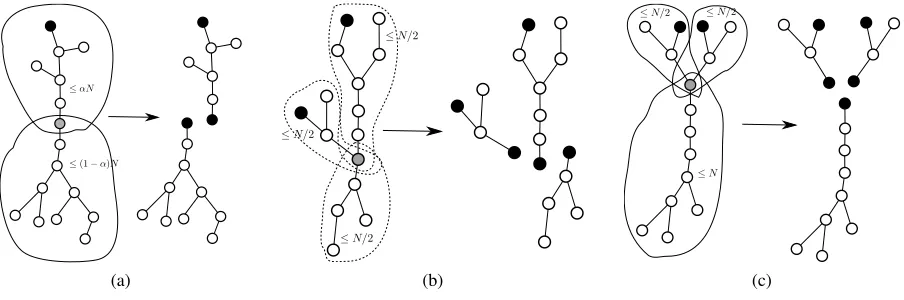
Figure 6: Choosing splitting node in three different cases. Rounding errors are ignored for simplicity.
Proof. Denote byT1(N),T2(N)the running time ofAlgorithm 4using splitting ruleH2ontype1ortype2 trees each ofNnodes respectively. Splitting atype1tree results in multipletype1trees with size at most
(1−α)Nand onetype2tree with size at mostαN, so we have
T1(N)≤O(d(1−ε)TW(φ)) (T1((1−α)N) +T2(αN)) +2O(TW(φ)).
Splitting atype2tree, when the 1/2-splitting is on the path betweenp1andp2results in twotype2trees with size at mostN/2 and multipletype1trees. Otherwise, the splitting operation results in twotype2 trees with size at mostN/2 and severaltype1trees. Hence:
T2(N)≤O(d(1−ε)TW(φ)) (T1(N) +T2(N/2)) +2O(TW(φ)).
Setα=3−
√
5
2 to minimize the values ofT1(N)andT2(N), we have
T1(N)≤O(d(1−ε)TW(φ)) (T1((1−α)N) +T2(αN)) +2O(TW(φ))
≤O(d(1−ε)TW(φ))T1((1−α)N) +O(d2(1−ε)TW(φ))T1(αN) +2O(TW(φ)).
Therefore:
T1(N)≤d
1
−log(1−α)(1−ε)TW(φ)logN|φ|O(1).
Sincetypei,i≥3 trees are not allowed, the space requirement is 22εTW(φ)|φ|O(1).
4.5 Optimality of the splitting algorithm for the single-parameter tradeoff
The splitting algorithm presented above is a specific one, with the property that it does not createtypei
trees for anyi≥3. Interestingly, it can be shown that this specific splitting algorithm is optimal over all splitting strategies which enjoy this property.
Definition 4.10. Denote by Ac (∀c≥2) the family of algorithms for SAT with bounded tree-width
following the framework inAlgorithm 3which use a splitting algorithm without creatingtypei trees
Algorithm 4H2(T,S)
1: ifTwithSis atype0treethen
2: returnthe 1/2-splitting node
3: else ifTwithSis atype1treethen
4: regard the previous splitting node as root
5: returntheα-splitting node .Figure 6a
6: else ifTwithSis atype2treethen
7: supposeS={p1,p2}
8: regard p1as root and compute the 1/2-splitting nodeq
9: ifqis on the path between p1andp2then
10: returnq .Figure 6b
11: else
12: returnthe least common ancestor ofqandp2 .Figure 6c
13: end if
14: end if
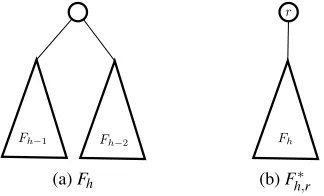
We lower bound the running time of all algorithms in A2 by showing hard instances based on generalizations of Fibonacci trees.
Definition 4.11. For any positive integerh, ah-Fibonacci tree(denoted asFh) is a rooted tree recursively
defined as following,
(1) ifh=1,Fhcontains only 1 node;
(2) ifh=2,Fhcontains 2 nodes and one edge between them;
(3) ifh>2,Fhis constructed by a root connecting roots of two subtreesFh−2andFh−1.
Anextended(h,r)-Fibonacci tree(denote asFh∗,r) is constructed by adding one edge between a root node rand the root of subtreeFh.
(a)Fh (b)Fh∗,r
Figure 7: Fibonacci tree and extended Fibonacci tree.
In what follows, we focus on the structure of the trees and inspect the running time of an algorithm in