Numerical solution of nonlinear fractional integro-differential equation by Collocation method

https://doi.org/10.26637/MJM0601/0011

Numerical solution of nonlinear fractional

integro-differential equation by Collocation method

S. I. Unhale

and S. D. Kendre

*

Abstract

In this paper, we presents the Collocation Method with the help of shifted Chebyshev polynomials and shifted Legendre polynomials for the numerical solution of nonlinear fractional integro-differential equations (NFIDEs). The method introduces a promising tool for solving many NFIDEs with the help of Newton’s iteration method. Keywords

Fractional Integrodifferential Equations, Collocation method, Chebyshev Polynomials, Legendre polynomials.

AMS Subject Classification

34A08, 65L05, 65L20

1_{Department of Mathematics, C.K. Thakur Arts, Commerce and Science College, New Panvel 410 206, India (M.S.)} 2_{Department of Mathematics, Savitribai Phule Pune University, Pune-411007, India (M.S.)}

*Corresponding author:2_{[email protected],}2_{[email protected];} 1_{[email protected]}

Article History: Received12October2017; Accepted26December2017 c2017 MJM.

Contents

1 Introduction. . . 73

2 Preliminaries and Definitions. . . 74

3 Solution of NFIDEs by Collocation method with the help of shifted Chebyshev polynomials. . . 74

4 Solution of NFIDEs by Collocation method with the help of shifted Legendre polynomials. . . 75

5 Applications. . . 76

6 Conclusion. . . 78

Acknowledgments. . . 79

References. . . 79

1. Introduction

It is now a days well established that several real life phe-nomena are better described by fractional differential equa-tions and hence the study of these type of equaequa-tions is very important due to their frequent appearance in various appli-cations in fluid mechanics, biology, physics and engineering see [1,2,4]. Most of the fractional differential equations do not have exact analytic solutions and therefore, approximating or numerical techniques are generally applied. Consequently, considerable attention has been given to the solutions of frac-tional differential equations and fracfrac-tional integral equations using different numerical methods such as Predictor Correc-tor method, Quadrature methods, Fractional Euler, Fractional

Trapezoidal method, Legendre spline interpolation method, Adomain decomposition method, Taylor series method, Pi-card’s iterative method, Variational principle method, Iterative methods, Laplace transform, Mellin transform, Collocation method, Galerkin method and many others. Many recent pa-pers have dealt with the solutions of fractional differential equations by using above methods, see [5–7,9,14,20,21] and some of the references cited therein.

As Chebyshev polynomials and Legendre polynomials are well known family of orthogonal polynomials on the interval

[−1,1]that have many applications and widely used because of their good properties in the approximation of functions. This motivated to find a numerical solution of nonlinear fractional integrodifferential equations using Collocation method with the help of Chebyshev polynomials and Legendre polynomials to reduce to system of nonlinear equations and which can be solved by Newtons Iterative method.

The aim of the present paper is to determine the numerical solution of the nonlinear fractional integrodifferential equation of the type

Dα_{y(x) =g(x) +}

Z 1

0

K(x,t)f(y(t))dt, (1.1)

y(i)(0) =δ(i), i=0,1, . . . , (1.2)

in the interval[0,1]andy(x)is the unknown function to be determined.

The paper is organized as follows: Section 2, presents the preliminaries and definitions. Section 3, dedicates the solution of nonlinear fractional integrodifferential equation by Colloca-tion method with the help of shifted Chebyshev polynomials. Section 4, obtains the solution of nonlinear fractional integrod-ifferential equation by Collocation method with the help of shifted Legendre polynomials. Section 5, focuses on some examples to illustrate the theory.

2. Preliminaries and Definitions

In this section we recall some definitions and properties of fractional derivatives and fractional integrals [13,16].

Definition 1. A real function f(x),x>0, is said to be in the space Cµ,µ∈R, if there exists a real number p>µsuch that

f(x) =xpf1(x), where f1(x)∈C[0,1).

Definition 2. A real function f(x),x>0, is said to be in the space Cm

µ,m∈NU{0}if and only if f (m)_∈C

µ.

Definition 3. The fractional integral of orderαwith the lower limit zero for a function f is defined as

Iα_{f(x) =} 1

Γ(α) Z x

0

f(t)

(x−t)1−αdt, x>0,α>0, (2.1)

provided the right side is point-wise defined on [0,∞), where Γ(·)is the gamma function.

Definition 4. The Riemann-Liouville derivative of orderα with the lower limit zero for a function f :[0,∞)→R can be written as

L_Dα_{f(x) =} 1

Γ(n−α) dn dxn

Z x

0

f(t)

(x−t)α+1−ndt,x>0, (2.2)

for n−1<α<n.

Definition 5. The Caputo derivative of orderαfor a function f :[0,∞)→R can be written as

Dα_{f(x) =}  



In−αfn(x), n−1<α≤n, n∈N, Dnf(x)

Dxn , α=n.

(2.3)

3. Solution of NFIDEs by Collocation

method with the help of shifted

Chebyshev polynomials

The well known Chebyshev polynomials are defined on the interval [−1,1] and can be determined with the use of the following recurrence formula

Tn(z) =2zTn−1(z)−Tn−2(z), n=2,3, . . .

with

T0(z) =1, T1(z) =z.

The analytic form of the Chebyshev polynomials Tn(z)of degreenis given by

Tn(z) =n [n₂]

∑

(−1)i2n−2i−1(n−i−1)!

(i)!(n−2i)!z

n−2i _(3.1)

where[n

2]denotes the integer part ofn/2.

The orthogonality condition is

Z 1

−1

Ti(z)Tj(z)

√

1−z2 dz=    

  

π, f or i=j=0;

π

2, f or i=j6=0; 0, f or i6= j.

(3.2)

In order to use these polynomials on the interval [0,1] we define the so called shifted Chebyshev polynomials by intro-ducing change of variablesz=2x−1. The shifted Chebyshev polynomialsTn(2x−1)be denoted byTn∗(x). ThenTn∗(x)can be obtained as follows

T_n∗(x) =2(2x−1)T_n−∗₁(x)−T_n−∗₂(x), (3.3) forn=2,3, . . .with initial conditions

T₀∗(x) =1, T₁∗(x) =2x−1. (3.4) The analytic form of shifted Chebyshev polynomialsT_n∗(x)of degree n is given by

T_n∗(x) =n

n

∑

(−1)n−k2

2k_(n+k−1)!

(2k)!(n−k)! x

k_{, (3.5)}

forn=2,3, . . .

The functiony(x), which is square integrable functions in[0,1], may be expressed in terms of shifted Chebyshev polynomials as

y(x) =

∞

∑

aiTi∗(x), (3.6)

where the coefficientsaiare given by

a0=

1

π Z 1

0

y(x)T₀∗(x)

√

x−x2 dx, ai=

2

π Z 1

0

y(x)T_i∗(x)

√

x−x2 dx,

for i=1,2, . . .. In practice, only the first (n+1)terms of shifted Chebyshev polynomials are considered. Then we have

yn(x)∼= n

∑

aiTi∗(x), 0≤x≤1. (3.7)

Theorem 3.1 (Chebyshev Truncation Theorem). [12] The error in approximating y(x)by the sum of its first n terms is bounded by the sum of the absolute values of all the neglected coefficients. If

yn(x)∼= n

∑

then

ET(n) =|y(x)−yn(x)| ≤ ∞

∑

|ak| (3.9)

for all y(x), all n and all x∈[−1,1].

The main approximate formula of the fractional derivative ofyn(x)is given in the following theorem.

Theorem 3.2. [12] Let y(x)be approximated by shifted Cheby-shev polynomials and also supposeα>0, then

Dα_(y n(x)) =

n

∑

i

∑

aiw (α) i,k x

k−α _(3.10)

where w(α)_i,k is given by

w(α)_i,k = (−1)i−k 2

2k_{i(i+k−1)!Γ(k+1)}

(i−k)!(2k)!Γ(k+1−α) (3.11) The numerical solution of nonlinear fractional integrodif-ferential equation (1.1) using collocation method with the help of shifted Chebyshev polynomials is discussed below. This method is based on approximating the unknown functiony(x)

as

yn(x)∼= n

∑

aiTi∗(x), 0≤x≤1 (3.12)

whereT_i∗(x)is the shifted Chebyshev polynomial andai, i= 0,1,2, . . .are constants.

Making use of (3.12) into (1.1), following equation is obtained

n

∑

i

∑

aiw(α)_i,k xk−α

=g(x) + Z 1

0

K(x,t)f(

n

∑

aiTi∗(t))dt (3.13)

We now collocate equation (3.13) at (n+1− dαe) points xp,p=0,1, . . .n− dαeas

n

∑

i

∑

aiw(α)_i,k xk−αp

=g(xp) +

Z 1

0

K(xp,t)f( n

∑

aiTi∗(t))dt (3.14)

for suitable collocation points we use roots of shifted Cheby-shev polynomialsT_n+∗_1−dαe(x).

Also substituting equation (3.12) in the initial condition (1.1), we have

n

∑

(−1)iai=0. (3.15)

From equation (3.14) and equation (3.15), we obtain(n+1)

system of nonlinear equations ina0,a1, . . . ,angiven by

F0(a0,a1, . . . ,an) =0

F1(a0,a1, . . . ,an) =0

.. .

Fn(a0,a1, . . . ,an) =0      

    

, (3.16)

which can be solved by using the Newton’s iteration method for system of nonlinear equation.

To develop the iterative scheme, the system of nonlinear equation (3.16) can be written in the vector form asF(a) =0,

wherea= (a0,a1, . . . ,an)andF= (F0,F1, . . . ,Fn). The Taylor series expansion is

F(ak+1) =F(ak) + (∂F ∂a)(a

k+1_−ak_{) +· · ·. (3.17)}

Truncating the Taylor’s series following equation is obtained

F(ak) + (∂F(a

k₎

∂a )(a

k+1_−ak_{) =0, (3.18)}

which gives

ak+1=ak−

∂F(ak)

∂a −1

F(ak) (3.19)

provided that the inverse of Jacobian Matrix ∂F(a k₎

∂a exists. First we solve the equation

∂F(ak)

∂a 4x=−F(a

k_{) (3.20)}

where

4x=ak+1−ak. (3.21)

Since ∂F(a k₎

∂a is a known matrix andF(a

k_{)is a known vector,}

the equation (3.20) is just a system of linear equations, which can be solved efficiently and accurately. Once we have the solution vector4x, we can obtain improved estimateak+1by equation (3.21).

4. Solution of NFIDEs by Collocation

method with the help of shifted Legendre

polynomials

The well known Legendre polynomials are defined on the interval [−1,1] and can be determined with the use of the following recurrence formula

Ln(z) = 2n+1

n+1 zLn−1(z)−

n

forn=2,3, . . .

with

L0(z) =1, L1(z) =z.

In order to use these polynomials on the interval[0,1], we define the so called shifted Legendre polynomials by intro-ducing change of variablesz=2x−1. The shifted Legendre polynomialsLn(2x−1)be denoted byLn∗(x). ThenL∗n(x)can be obtained as follows

L∗_n(x) =(2n+1)(2x−1) n+1 L

∗ n−1(x)−

n (n+1)L

∗

n−2(x), (4.1)

forn=2,3, . . .

with initial conditions

L∗₀(x) =1, L∗₁(x) =2x−1. (4.2) The analytic form of shifted Legendre polynomialsL∗_n(x)of degreenis given by

L∗_n(x) =

n

∑

(−1)n+i (n+i)! (n−i)((i)!)2x

i_{, n=2,3, . . . (4.3)}

The orthogonality condition is

Z 1

0

L∗_i(x)L∗_j(x)dx=  

 1

2i+1, f or i=j; 0, f or i6=j.

(4.4)

The functiony(x), which is square integrable in[0,1], may be expressed in terms of shifted Legendre polynomials as

y(x) =

∞

∑

aiL∗i(x), (4.5)

where the coefficientsaiare given by

ai= (2i+1)

Z 1

0

y(x)L∗_i(x)dx, i=0,1,2, . . .

In practice, only the first(n+1)terms of shifted Legendre polynomials are considered. Then we have

yn(x)∼= n

∑

aiL∗i(x). (4.6)

The main approximate formula of the fractional derivative of

yn(x)is given in the following theorem.

Theorem 4.1. [3] Let y(x)be approximated by shifted Legen-dre polynomials and supposeα>0

Dα_(y n(x)) =

n

∑

i

∑

aiw(α)_i,k x

k−α _(4.7)

where w(α)_i,k is given by

w(α)_i,k = (−1)i+k (i+k)!Γ(k+1)

(i−k)!(k!)2_Γ(k+1−α) (4.8)

The numerical solution of nonlinear fractional integrod-ifferential equation (1.1) using collocation method with the help of shifted Legendre polynomials is discussed below. This method is based on approximating the unknown functiony(x)

as

yn(x)∼= n

∑

aiL∗i(x), 0≤x≤1 (4.9)

whereL_i∗(x)is the shifted Legendre polynomial. Using (4.9) in (1.1), we obtain

n

∑

i

∑

aiw (α) i,k x

k−α

=g(x) + Z 1

0

K(x,t)f(

n

∑

aiL∗i(t))dt (4.10)

Now we collocate equation (4.10) at(n+1− dαe) points xp, p=0,1,· · ·n− dαeas

n

∑

i

∑

aiw(α)_i,k xk−αp

=g(xp) +

Z 1

0

K(xp,t)f( n

∑

aiL∗i(t))dt. (4.11)

For suitable collocation points we use roots of shifted Legendre polynomials L∗_n+1−dαe(x)and the initial condition (1.1), we obtain(n+1)system of nonlinear equations ina0,a1, . . . ,an. These system of nonlinear equations can be solved by using the Newton’s iteration method discussed above section.

5. Applications

In this section, we give some numerical examples of nonlinear fractional integrodifferential equations to illustrate the above results.

Example 5.1. Consider the following nonlinear fractional integrodifferential equation

Dα_{y(x) =1−}1 4x+

Z 1

0

xt(y(t))2dt, (5.1)

y(0) =0. (5.2)

where0≤x<1, α=1₂. The differential equation (5.1)-(5.2) has the exact solution y(x) =x,ifα=1.

Method I: Collocation method with the help of shifted Chebyshev polynomials

The suggested method is implemented forn=3 and approxi-mate the solution as follows

y2(x)∼= 3

∑

aiTi∗(x), 0≤x≤1. (5.3)

An application of Collocation method with the help of shifted Chebyshev polynomial to (5.1)-(5.2), following nonlinear sys-tem of equations is obtained,

F0(a0,a1,a2,a3) =−0.25a20−0.166667a1a0 +0.166667a2a0+0.1a3a0

−0.0833333a2₁−0.116667a2₂

−0.121429a2₃+1.59577a1

−0.0333333a1a2−2.12769a2 +0.1a1a3−0.0714286a2a3

−0.957461a3−0.875

F1(a0,a1,a2,a3) =−0.0334936a2₀−0.0223291a1a0 +0.0223291a2a0+0.0133975a3a0

−0.0111645a2₁−0.0156304a2₂

−0.0162683a2₃+0.584092a1

−0.00446582a1a2−2.12769a2 +0.0133975a1a3−0.00956961a2a3 +4.07187a3−0.983253

F2(a0,a1,a2,a3) =−0.466506a20−0.311004a1a0 +0.311004a2a0+0.186603a3a0

−0.155502a2₁−0.217703a2₂

−0.226589a2₃+2.17986a1

−0.0622008a1a2+2.12769a2 +0.186603a1a3−0.133288a2a3 +3.11441a3−0.766747

F3(a0,a1,a2,a3) =a0−a1+a2−a3.

Using Newton’s iteration method for nonlinear system of equa-tions, we obtain

a0=0.832197311166694

a1=0.5989063759298973

a2=−0.14392391710534502

a3=0.08936701813145172,     

   

(5.4)

making use of the (5.4) into (5.3), following solution is ob-tained

y(x) =0.83219731+0.5989063759298973(2x−1)

−0.14392391(8x2−8x+1)

+0.089367(4(2x−1)3−3(2x−1)), (5.5)

which is approximate solution of (5.1)-(5.2).

In Figure 1, we plot the approximate solution obtained by Method I and the exact solution for Example5.1.

Figure 1.Approximate and Exact solution of Example 5.1 by Method I

Method II: Collocation method with the help of shifted Legendre polynomials

The suggested method is implemented forn=3 and approxi-mate the solution as follows

y2(x)∼= 3

∑

aiL∗i(x), 0≤x≤1. (5.6)

whereL∗_i(x)is the shifted Legendre polynomial andai, i= 0,1,2,3 are constants.

An application of Collocation method with the help of shifted Legendre polynomials to (5.1)-(5.2), following nonlinear sys-tem of equations is obtained,

F0(a0,a1,a2,a3) =−0.25a20−0.166667a1a0

−0.0833333a2₁−0.05a2₂

−0.0357143a2₃+1.59577a1

−0.0666667a1a2−1.59577a2

−0.0428571a2a3+1.88411095∗10−15a3

−0.875

F1(a0,a1,a2,a3) =−0.0563508a20−0.0375672a1a0

−0.0187836a2₁−0.0112702a2₂

−0.00805012a2₃+0.757618a1

−0.0150269a1a2−1.93131a2

−0.00966a2a3+2.99198a3−0.971825 F2(a0,a1,a2,a3) =−0.443649a20−0.295766a1a0

−0.147883a2₁−0.0887298a2₂

−0.0633785a2₃+2.12579a1

−0.118306a1a2+1.16747a2

−0.076054a2a3+1.8086a3−0.778175

F3(a0,a1,a2,a3) =a0−a1+a2−a3

Using Newton’s iteration method for nonlinear system of equa-tions, we obtain

a0=0.7765706927568846

a1=0.5681834659041213

a2=−0.12918879599732455 a3=0.07919843085543878

    

   

making use of (5.7) into (5.6), following solution is obtained

y(x) =0.776571+0.568183(2x−1)

−0.129189(6x2−6x+1)

+0.0791984(20x3−30x2+12x−1) (5.8) which is approximate solution of (5.1)-(5.2).

In Figure 2, we plot the approximate solution obtained by Method II and the exact solution for Example5.1.

Figure 2.Approximate and Exact solution of Example 5.1 by Method II

Example 5.2. Consider the following nonlinear fractional integrodifferential equation

Dα_{y(x) =}

8x3/2

3 −2

√

x

√

π −

1 1260x+

Z 1

0

xt(y(t))4dt,

(5.9)

y(0) =0. (5.10)

where0≤x<1,α=1₂. The differential equation (5.9)-(5.10) has the exact solution y(x) =x2_−x,ifα=1.

Method I: Collocation method with the help of shifted Chebyshev polynomials

Similarly as in Example 5.1 applying the Collocation method with the help of shifted Chebyshev polynomial to (5.9)-(5.10), we obtain,

a0=−0.12500000268834607 a1=−3.2462632438396387∗10−9 a2=0.12499999951591143

a3=7.382860772130038∗10−11      

    

(5.11)

Hence the approximate solution of (5.9)-(5.10) is

y(x) =−0.125−3.24626∗10−9(2x−1) +0.125(8x2−8x+1)

+7.38286∗10−11(4(2x−1)3−3(2x−1)).

(5.12)

In Figure 3, we plot the approximate solution obtained by Method I and the exact solution for Example5.2.

Figure 3.Approximate and Exact solution of Example 5.2 by Method I

Method II: Collocation method with the help of shifted Legendre polynomials

Similarly as in Example 5.1 applying the Collocation method with the help of shifted Legendre polynomial to (5.9)-(5.10), we obtained,

a0=−0.16667380012560998 a1=3.971261224148561∗10−6 a2=0.16667060752789342

a3=−7.16385894071834∗10−6      

    

(5.13)

Hence the approximate solution of (5.9)-(5.10) is

y(x) =−0.166674+3.97126∗10−6(2x−1) +0.166671(6x2−6x+1)

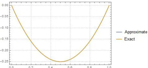
−7.16386∗10−6(20x3−30x2+12x−1). (5.14) In Figure 4, we plot the approximate solution obtained by Method II and the exact solution for Example5.2.

Figure 4.Approximate and Exact solution of Example 5.2 by Method II

6. Conclusion

and Legendre polynomials are used to reduce nonlinear frac-tional integrodifferential equation to the solution of system of algebraic equations. The solution obtained using this method is in excellent agreement with the exact solution and show that this method is effective.

All numerical results are obtained using Mathematica 11.

Acknowledgments

The authors would like to express sincere gratitude to the reviewers for his/her valuable suggestions.

References

[1] _{G. Adomain; Solving Frontier Problems of Physics: The}

Decomposition Method,Kluwer, Boston, (1994). [2] _{G. Adomain; A review of the decomposition method in}

applied mathematics,J. Math. Anal. Appl., 135 (1988), 501-544.

[3] _{Rubayyi T. Alqahtani; Approximate Solution of non-linear}

fractional Klein-Gordon equation using Spectral Colloca-tion mehtod,J. Appl. Math., 6 (2015), 2175-2181. [4] _{R.L. Bagley and P.J. Torvik, A theoretical basis for the}

application of fractional calculus to viscoelasticity,J. Rhe-ology, 27(3), (1983), 201-210.

[5] _{X. Cao and Y. Li; Fractional Runge-Kutta methods for}

nonlinear Fractional differential equations,J. Nonl. Syst. Appl.(2011), 189-194.

[6] _{V. Daftardar-Gejji and H. Jafari; Adomian}

decomposi-tion: a tool for solving a system of fractional differential equations,J. Math. Anal. Appl., 301 (2005), 508-518. [7] _{V. Daftardar-Gejji and H. Jafari; An iterative method for}

solving nonlinear functional equations, J. Math. Anal. Appl., 316 (2006), 753-763.

[8] _{K. Diethelm and Yu. Luchko, Algorithms for the fractional}

calculus: A selection of numerical methods,J.Comput. Methods Appl. Mech. Eng., 194, (2005), 743-773. [9] _{E. A. Ibijola and B. J. Adegboyegun; A comparison of}

Adomain’s decomposition method and Picard iterations method in solving nonlinear differential equations,Global J. Sci. Frontier Research Math. Deci. Sci., 12 (7), (2012). [10] _{A. Kadem and D. Baleanu, Fractional radiative}

trans-fer equation within Chebyshev spectral approach, J. Compu.and Math. with Appl., 59, (2010), 1865-1873. [11] _{M. M. Khader and A. S. Hendy, The approximate and}

exact solutions of the fractional order delay differential equations using Legendre pseudospectral method,Int. J. Pure and Appl. Math., 74(3),(2012), 287 – 297.

[12] _{M. M. Khader, N. H. Sweilam and A. M. S. Mahdy,}

Nu-merical study for the fractional differential equations gen-erated by optimization problem using Chebyshev colloca-tion method and FDM,J. Appl. Math. and Info. Sci., 7(5), (2013), 2011-2018.

[13] _{A. A. Kilbas, H. M. Srivastava and J. J. Trujillo; Theory}

and applications of fractional differential equations,

North-Holland Mathematics Studies, vol. 204, Elsevier Science B. V., Amsterdam, (2006).

[14] _{D. Sh. Mohammed; Numerical solution of fractional}

integrodifferential equations by Least squares method and shifted Chebyshev polynomial,Math. Probl. Engg., (2014),1-5.

[15] _{Necati Ozisik; Finite Difference Methods in Heat Transfer}

CRC Press, (1994).

[16] _{I. Podlubny; Fractional differential equations,Academic}

Press, San Diego, (1999).

[17] _{E.A. Rawashdeh, Numerical solution of fractional}

integro-differential equations by collocation method,J. Appl. Math. Comput., 176, (2006), 1-6.

[18] _{M. A. Snyder, Chebyshev Methods of Partial Differential}

Equations, Oxford University Press, (1965).

[19] _{S. Momani, M.A. Noor, Numerical methods for}

fourth-order fractional integro-differential equations, Appl. Math. Comput., 182, (2006), 754-760.

[20] _{Abdul-Majid Wazwaz; Linear and Nonlinear Integral}

equations, Methods and Applications,Springer, (2011). [21] _{C. Yang and J. Hou; Numerical solution of}

integrodiffer-ential equations of fractional order by Laplace decomposi-tion method,Wseas Transactions on Mathematics,12 (12), (2013), 1173-1183.

? ? ? ? ? ? ? ? ?

ISSN(P):2319−3786

Malaya Journal of Matematik

ISSN(O):2321−5666