Abstract— The paper aims at detecting on-line cognitive failures in driving by decoding the EEG signals acquired during visual alertness, motor-planning and motor-execution phases of the driver. Visual alertness of the driver is detected by classifying the pre-processed EEG signals obtained from his pre-frontal and frontal lobes into two classes: alert and non-alert. Motor-planning performed by the driver using the pre-processed parietal signals is classified into four classes: braking, acceleration, steering control and no operation. Cognitive failures in motor-planning are determined by comparing the classified motor-planning class of the driver with the ground truth class obtained from the co-pilot through a hand-held rotary switch. Lastly, failure in motor execution is detected, when the time-delay between the onset of motor imagination and the EMG response exceeds a predefined duration. The most important aspect of the present research lies in cognitive failure classification during the planning phase. The complexity in subjective plan classification arises due to possible overlap of signal features involved in braking, acceleration and steering control. A specialized interval/general type-2 fuzzy set induced neural classifier is employed to eliminate the uncertainty in classification of motor-planning. Experiments undertaken reveal that the proposed neuro-fuzzy classifier outperforms traditional techniques in presence of external disturbances to the driver. Decoding of visual alertness and motor-execution are performed with kernelized support vector machine classifiers. An analysis reveals that at a driving speed of 64 km/hr, the lead-time is over 600 milliseconds, which offer a safe distance of 10.66 meters.
Index Terms— EEG, Visual alertness, planning, Motor-execution and Type-2 fuzzy classifiers.
I. INTRODUCTION
Driving involves complex cognitive processes, concerning sensory perception, motor-planning and motor-execution. The cognitive failure detection (CFD) problem, introduced here, refers to classifying cognitive failures involved in visual alertness (VA), motor-planning (MP) and motor-execution (ME) phases of driving with a motive to alert the driver by an (audio) alarm before an accident takes place. One approach to solve the above problem is to capture the brain signals of the driver by a non-invasive means for subsequent processing and classification.
Among the well-known brain signal acquisition techniques, electroencephalography (EEG) [1] is most popular for its prompt time-response [2], non-invasive characteristic [3], [4] portability and cost-effectiveness. Because of the above merits, the paper attempts to employ EEG-signal processing and classification to detect VA failure (VAF), MP failure (MPF) and ME failure (MEF). The VAF is recognized from the acquired P-300 response of the driver in reaction to
external stimulation [5]-[8], such as sudden appearance of bumpers, traffic light changes, and the like. MPF and MEF
detection, require Event Related
De-synchronization/Synchronization (ERD/ERS), which, being spontaneous, requires no external stimulation for its generation [5], [6].
Classification of cognitive tasks from the acquired EEG signals is relatively easier when the tasks involve disjoint brain regions. However, cognitive tasks (braking, acceleration and steering control) involved in MP usually engage the same cortical regions (parietal and motor cortex), with an overlap in their feature space. This overlap acts as a source of uncertainty to the classifier. Traditional classifiers, which usually show promising performance, unfortunately, fail to accurately discriminate pattern classes with overlapped features. The logic of fuzzy sets has an inherent power to handle uncertainty in measurement space. Thus fuzzy logic induced classifiers are a good choice for the present MP classification. Our experience [9]-[12] further reveals that the MP features of the above three cognitive tasks have wider fluctuations over experimental instances of the same subject and across subjects. Type-2 fuzzy set has an added advantage over its type-1 counterpart to handle both intra- and inter-personal level uncertainty [13].This motivated us to employ Interval type-2 Fuzzy sets/General type-2 Fuzzy sets (IT2FS/GT2FS) [14] to design classifiers for the MP classes.
There exist traces of works on pattern classifiers using type-2 fuzzy sets. Das et al. employed projection-based learning techniques to determine optimal weights of a multilayered type-2 neuro-fuzzy classifier [15]. Lee et al.
introduced a recurrent interval type-2 fuzzy neural net (IT2FNN) for non-linear system identification. They employed asymmetric interval type-2 membership functions for type-2 fuzzy reasoning, and used gradient descent learning for weight adaptation [16]. Lin et al. in [17], proposed a self-organizing model of IT2FNN, where the motivation is to employ i) self-organized learning for the determination of fuzzy rules and ii) parameter learning for the selected fuzzy rules. In the self-organized learning phase, new type-2 rules are added and inefficient rules are pruned out of the IT2FNN. In [18], Park et al. introduced a new model of IT2FNN where type-2 fuzzy rules include a function of the linguistic variables in the consequent. The fundamental aspect of their work lies in automatic tuning of parameters of the IT2FNN using real-coded Genetic Algorithm.
Current research on type-2 classifiers is primarily focused around adding sophisticated learning paradigms to improve classifier performance. The new learning paradigms introduced include extreme learning machines [19], active/incremental learning [20], [21], transfer learning [22],
EEG-Analysis for Cognitive Failure Detection
in Driving Using Type-2 Fuzzy Classifiers
[23] and multi-view learning [24] techniques. For example,
Deng et al. employed extreme learning algorithm to adapt parameters in the consequent of type-2 fuzzy rules to improve generalization performance of the resulting system [19]. Pratama et al. also addressed techniques for generalization and summarization capability of IT2FS classifier by introducing learning mechanisms to expand, prune, recall and merge rules [25]. Yang et al. utilized transfer learning principles [22] in Takagi-Sugeno fuzzy logic systems for adaptive recognition of epileptic EEG signals [23]. In [20], [21] the authors proposed two interesting works on incremental type-2 meta-cognitive learning machines that autonomously detect what, how and when to learn.
In recent times, an increasing interest to classify brain signals is noticed in research community [26], [27]. For example, Wang et al. selected random forest algorithm for epilepsy detection for its superior performance over its three competitors, including decision tree and support vector machine (SVM) based realizations of both decision tree and random forest [28]. Herman et al. [29] examined the scope of IT2FS induced classifier in motor imagery related EEG classification task for both off-line and online test cases. In [30], the authors indicated that type-2 fuzzy logic classifier outperforms the traditional linear discriminant analysis (LDA) classifier in terms of classification accuracy in presence of noise. Nguyen et al. proposed a novel approach for motor imagery classification using wavelet feature induced interval type-2 fuzzy classifier [31] and demonstrated that the said classifier outperforms traditional statistical, neural and adaptive neuro-fuzzy inference system (ANFIS) classifiers. Andreu-Perez et al. proposed a self-adaptive GT2FS-induced inference system for online classification of motor imagery to navigate a bi-pedal humanoid robot [32].
Traditional type-2 fuzzy inference generating systems usually employ rules with type-2 fuzzy propositions in the antecedent and type-2/interval type-1 fuzzy propositions in the consequent [15], [33]-[37]. The classifier rules employed in this paper are designed with type-2 fuzzy propositions to synthesize the antecedent and a single crisp class label at the consequent. The intra- and inter-subjective variations in the acquired brain signals are accommodated in the construction of type-2 membership functions (MFs) of the antecedent propositions. The crisp, instead of interval type-2, class label is used in the consequent to describe precise/hard classification of MP tasks in presence of imprecise measurements.
In this paper, two different proposals for type-2 classifiers are introduced, one synthesized with interval type-2 (IT2) and the other with general type-2 (GT2) fuzzy neural networks. Both the realizations include two layered neural nets with the first layer performing IT2/GT2 fuzzification [13], firing interval computation [15] and Nie-Tan type-reduction [15], [38], [39]. We here do not require defuzzification, as the class label of the input fuzzified features is determined by comparison of the type-reduced outputs of the neurons in the first layer. The second layer selects the neuron with the highest type-reduced output in the first layer and generates a decoded output pattern corresponding to the position of the selected neuron in the first layer. Since defuzzification is avoided and Nie-Tan type-reduction involves only averaging
operation, the run-time complexity of the classifiers is reduced significantly, making them amenable for real-time driving application.
In addition, the GT2 classifiers proposed here utilize a novel technique for secondary MF evaluation. Here, the secondary MF at a given value of the linguistic variable
x
x
and primary membership A( )x in fuzzy setA
is obtained based on the location of the optima of
A( )
x
overx
, and the distance ofx
from its two neighborhood optima on its both sides. The computation of secondary membership is done offline to reduce run-time complexity of the classifiers. It may be noted that in traditional z-sliced based GT2 system [40], the GT2MF is presumed to have a specific geometry, such as triangle. The proposed method, on the other hand, computes secondary MF from the primary MF and thus is more accurate. Computational complexity of the proposed GT2FS-induced classifier also is nominal as it requires m.d extra multiplications in comparison to the proposed IT2FS induced classifier, where d denotes the number of GT2FS used in the antecedent of a rule and m denotes the number of rules used.The novelty of the paper thus lies in the design of an integrated CFD system for driving applications with special emphasis to the design of a fast and accurate type-2 (IT2FS/GT2FS) classifier to classify the MP classes, including braking (BR), acceleration (ACC), steering (STR) control and no operation (NOP). Besides CFD system and type-2 neuro-fuzzy classifier design, the other original contribution of the paper lies in the design of an evolutionary feature selection algorithm. This algorithm is used to reduce dimension of EEG-features for subsequent classification of MP and ME signals. The work presented here is significantly different from the authors’ previous works [9]-[12] with respect to formulation, approach and experiments.
The rest of the paper is structured as follows. In section II, we propose a psychological model of CFD cycle and present an integrated approach to system design for CFD. Section III describes evolutionary feature selection algorithm. In section IV, we emphasize the design of the proposed type-2 (IT2FS/GT2FS) classifiers as well as the kernelized SVM (KSVM) classifier. Section V is developed to deal with psycho-physiological experiments concerning selection of EEG filter bands, active brain regions and EEG features. In Section VI, we validate classifier performance, estimate lead-time for different speeds and evaluate objective performance of the proposed CFD system. Section VII offers classifier validation using McNemar’s test. Concluding remarks are given in section VIII.
II. SYSTEM DESIGN AND INTEGRATION
the driver. Fig. 1 provides a schematic representation of the cognitive failure detection loop, where VAF, MPF and MEF are monitored sequentially by the proposed system to generate necessary audio alarms to alert the driver. A commonsense thinking reveals that VAF may in turn result in MPF, which subsequently may result in MEF. In Fig. 1, we, however, attempt to identify the first occurrence of only one cognitive failure in the loop, rather than generating audio alarms for sequential failures, to avoid confusion of the driver.
In order to detect the above three cognitive failures of the driver, we need to process EEG signals from four distinct brain regions, including pre-frontal and frontal regions for testing VA, parietal lobe for MP and motor cortex region for ME. The acquired EEGs from pre-frontal/frontal, parietal and motor cortex regions are pre-processed using band pass filters (BPFs) of suitable frequency bands. VA being more prominent in alpha band (~8-13 Hz) [41] and MP/ME being relatively more active in mu- (8-13 Hz) [42] and beta (13-30 Hz) [43] bands, we used BPFs of required pass bands. More review on EEG channel selection and frequency band selection are provided in [44], [45]. Subsequent steps undertaken on the filtered signals include feature extraction, feature selection and classification.
For VAF, we require feature extraction and classification only as VAF can be characterized by fewer features. The importance of the VAF classifier is to detect the presence/absence of the P300 oddball signal within a finite interval of approximately 350 milliseconds. The classifier should recognize the visual non-alertness of the subject in absence of the P300. For MPF and MEF, we, require all the three steps: FE, FS and classification. Here, the classifier aims at detecting ERD/ERS from the parietal lobe within a specific time-period of approximately 600 milliseconds from the onset of the stimulus. It may be noted that although we count the time-point of ERD/ERS generation from the onset of the stimulus, such generation is spontaneous and is not directly influenced by the stimulus. In addition, MPF detection requires the ground truth (GT) planning decision from a second user, usually the co-pilot. The response of the MPF classifier is compared with the GT decisions to determine any subjective error of the pilot. Lastly, for the MEF detection, the classifier looks for the presence or absence of an ERD/ERS signal from the motor cortex.
If no ERD/ERS is detected within 800 milliseconds from the onset of the stimulus, the classifier declares the failures in motor execution. To confirm the MEF, we also pre-process,
filter and classify the elecctromyogram (EMG) signal acquired from the fore-arms/leg muscles of the subject. If no EMG signal is detected within 1200 milliseconds from the onset of the stimulus, the subject must have committed a fatal execution error. The above measurements are referred to driving speed above 64 km/hour. If driving speed falls off, the subject is relaxed and the above time markers shift right depending on the speed.
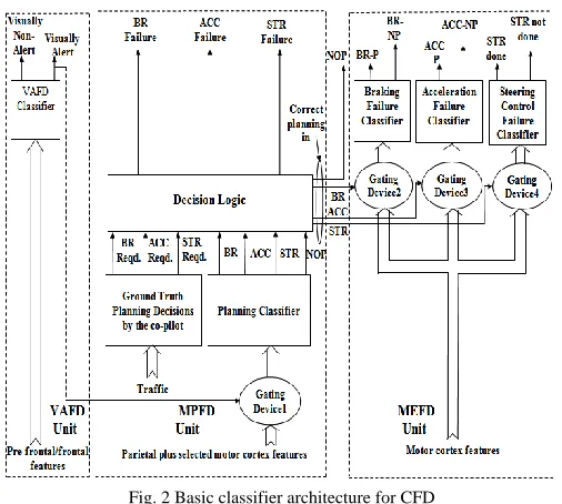
Fig. 2 includes three classifiers for VAF detection (VAFD), MPF detection (MPFD) and MEF detection (MEFD) and their interconnections. The VAFD classifier has two outputs: visually alert and non-alert. The MPFD classifier classifies planning failures into four classes: BR, ACC, STR and NOP. The MEFD unit includes three classifiers to classify ACC, BR and STR control failures during ME phase. The class labels of BR classifier are BR-pressed (BR-P) and BR-not pressed (BR-NP). Similar nomenclature is used for other two classifier outputs.
The planning classifier is structurally more complex than the rest as it needs to compare the detected class labels of the driver with the GT classes. The GT class labels are obtained from the co-pilot, who continuously feeds his decisions about the requirement of BR, ACC and STR control to the decision logic (Fig. 2) using a digital rotary switch. Since there are four possible classes (BR, ACC, STR and NOP), the co-pilot keeps the rotary switch in NOP mode unless any change is required at any point of time. After the co-pilot informs his planning decisions by pressing the right switch for ACC, BR and STR, it naturally returns to NOP by mechanical spring action. So, each planning decision may be regarded as a short duration pulse. The following two criteria have been used to select the co-pilot to assist a given pilot.
(1) The co-pilot’s response time of generating Event Related Potential should be to that of the main pilot, and (2) The co-pilot and the main pilot should be able to receive
stimuli concurrently without any interruptions.
The decision logic unit compares the parietal classifier response with the GT classes obtained from the co-pilot and
Fig. 1 Proposed psychological model of cognitive failure detection in driving to appropriately alert the driver with different audio alarms
thus determines appropriate planning failures in case there is a mismatch between the two responses (Fig. 3). Side connections from one classifier to the next in Fig. 2 are used to realize asynchronous operations between two successive classifiers. For example, if the subject is visually alert, we use this signal to act as a control input of a gating device to pass on parietal features to the MPFD classifier. Similarly, if no errors in BR, ACC and STR control signals are detected in MP phase, we use these signals as the control input of respective gating devices for subsequent BR, ACC and STR control classifiers during the ME phase.
III. FEATURE SELECTION
In the proposed CFD system, we used adaptive autoregressive (AAR) parameters for VAFD, power spectral density (PSD) and db4 wavelet coefficients for MPFD and MEFD. We selected these features based on our previous experience of working with EEG-based driving [9]. The AAR parameters being of low dimensions require no feature selection. However, PSD and DWT [46] features used in MP and ME having large dimensions require reducing features using a feature selection algorithm.
Let,
,1 ,2 ,
{ , , , }
k k k k
i i i i D
F f f f be the i-th feature vector with component fik,j, j 1 to D falling in the k-th class, where, i[1, ]n and k[1, ]m are positive integers,
c
kj andl j
c
be the j-th component of the cluster centers(geometric centroids) for the classes k and l respectively. Then the aim of the proposed feature selection algorithm is to select d<<D number of features in a manner such that it satisfies the following two objectives jointly.
(1) The first objective function J1 aims at minimizing the
city-block distance of all components of the i-th feature
vector, i[1, ]n from their respective cluster centers. This is ensured by minimizing (1).
1 ,
1 1 1
| |
m n D
k k
i j j k i j
J f c
(2) The second objective function J2 aims at maximizing the
distance between the cluster centers
c
kj and lj
c
of two classes k and lrespectively. This is realized with maximization of (2).2
1 1 1
| |
m m D k l j j l k j
l k
J c c
The two objective functions can be jointly represented by a composite objective function, given in (3), which needs to be minimized to attain the above two objectives satisfactorily.
1 2
,
J J
J
where, is a small positive number (0.001 say). The trial solutions here are binary strings of D-dimension representing presence or absence of a feature in the feature-vector. DE/rand/1/bin variation of Differential evolution (DE) [45] is used to obtain optimal solution (i.e., a binary string of D -dimension for which J is minimum) for the given minimization problem. Pseudo code for feature selection using DE is given in [47].
IV. CLASSIFIER SELECTION AND DESIGN
The VAFD and the MEFD classifiers are selected from the standard off-the-shelf classifiers as they have only two class labels. Here, because of superiority of KSVM in classification of non-linearly separable data-points [48], [49], we selected it for VAFD and MEFD classification.
The MPFD classifier has four classes: BR, ACC, STR and NOP, which are often found to have overlaps in feature space because of commonality of signal sources (here, motor cortex). This makes MPFD classification hard, leaving little space for traditional classifiers for the present application. Here, we need to design a suitable classifier, capable of performing classification with high accuracy at low computational overhead for real-time application. Fuzzy classifiers, in particular, type-2 fuzzy classifiers can serve the said purpose for their inherent capability to perform classification with overlapped class boundaries.
The existing IT2FS induced neural classifiers [15]-[18] show good performance with respect to classification accuracy, but their use for the present application is restrictive for their large computational overhead. This motivated us to design a simpler classifier with small computational overhead for real time application, however, without a compromise in their classification accuracy. In this section we would address two such fast classifiers, one realized with IT2FS- and the other using induced neurons. The proposed GT2FS-induced classifier has relatively better classification accuracy than its IT2FS counterpart, but the computational speed-wise IT2FS outperforms all existing and also the proposed GT2FS-induced neural net (GT2FS-NN) classifiers.
A. Preliminaries on Interval-Valued, IT2FS and GT2FS Definition 1: Let,Xbe the universe of discourse of a linguistic variable
x
. A classical (type-1) fuzzy setA
, defined on the universeX, is a two-tuple, given by} |
)) ( ,
{(x x x X
A A where, A(x), called membership of
x
in A, is a crispnumber in [0, 1] for any xX . The fuzzy set
A
is also expressed as( ) | A x X
A x x
where represents the union of all feasible xX[50].
Definition 2: Given a universe of discourseX
for the linguistic variablex
. Let, L([0,1])denote the set of all closed sub-intervals in [0,1] and is given byL([0,1]){x[ , ] | ( , )x x x x [0,1]2 and xx}. (6) An interval-valued fuzzy set A[51], [52] is given by a mapping
: ([0,1])
A X L , (7) and the membership degree of
x
X
is given by( ) [ ( ), ( )] ([0,1])
A x A x A x L , where A X: [0,1]and
: [0,1]
A X are mapped as the lower and the upper bound of the membership interval A x( ) respectively.
Definition 3: For a given universe of discourse
X
for the linguistic variablex
, a type-2, also called general type-2 fuzzy set (GT2FS)A
~
is a two-tuple [14], given by]} 1 , 0 [ , | )) , ( ), , {(( ~ ~
xu A xu x X u Jx
A
where,
) (
~ x
u
A (called primary membership) is a crisp number in [0, 1],] 1 , 0 [ ) , (
~ xu
A
is the secondary or type-2membership function (MF). The fuzzy set
A
~
is also expressed as] 1 , 0 [ ), , ( | ) , ( ~ ~
X x
x u J A
J u x u x A x ] 1 , 0 [ , | ] / ) ( [
X x
x u J x
J x u u f x where, f (u) ~(x,u) [0,1]
A
x
, and represents theunion over all feasible xXand uJx.
Definition 4: For a given xx,the 2-dimensional plane containing
u
and ( , )x u is referred to as vertical slice of) , (
~ x u
A
. Thus,
A( , ) x( ) | , x [0,1] u J x
x u f u u J
,
here, fx( )u lies in [0,1]. The amplitude of a secondary MF is
referred to as secondary grade of membership [13].
Definition 5: IfA( , )x u 1, x X and u Jx[0,1], then the type-2 fuzzy set Ais called an interval type-2 fuzzy
set (IT2FS). In other words, if all the secondary grades of a type-2 fuzzy set are equal to one, it is called as IT2FS [52].
Definition 6: An IT2FS contains an infinite number of
embedded type-1 fuzzy sets. The upper membership function (UMF) of an IT2FS is given by
A( ) ( Ae( )),
e
x Max x x
where, Aeis an embedded fuzzy set in the IT2FS.
Similarly the lower membership function (LMF) of an IT2FS is given by
( ) ( Ae( )), .
A
e
x Min x x
An IT2FS thus is bounded by an UMF and an LMF. The union
of all the embedded fuzzy sets in an IT2FS is called the
footprint of uncertainty (FOU) [13].
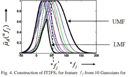
Let, fjbe a linguistic variable representing an experimental feature and A be a fuzzy set, representing CLOSE-TO-CENTRE-OF-THE-SPAN-OF-fj. Because of difference in experimental readings of the feature fj,we describe it by a Gaussian MF with mean and variance equal to their respective values of the feature in different experiments for the same subject. Thus, for 10 experimental subjects, we have 10 type-1 Gaussian MFs describing the statement: fj is A. We take the maximum and minimum of the 10 type-1 MFs to construct an IT2FS, where the maximum and minimum return the UMF and the LMF respectively (Fig. 4).
For multi-class classification using IT2FS, we use type-2 classifier rule i of the form: If f1 is A1and f2 isA2 and and
d
f is Ad, then class is Ci, where f1, f2, …, fd are d features
and Aj for j= 1 to d are IT2FS, and Ci is the i-th class label.
Now, for unknown measurements f1 f1 and f2 f2,…, ,
d d
f f we determine the firing strength of the rule i by taking the average of upper and lower firing strengths UFSi
and LFSi, where
2 1 1 2
( ( ), ( ), , ( ))
d
i A A A d
UFS Min f f f
(14)
and
1 1 2 2
( ( ), ( ), ( ))
d
i A A A d
LFS Min f f f (15) where j A and j A
are UMF and LMF of IT2FSAj.
Now, for k classifier rules, we say that the features:
1 1,
f f f2 f2,…, fd fd fall in class r if the average of LFSrand UFSr exceeds the average of LFSiand UFSi, i.
The justification of the averaging is briefly discussed below. It is important to note that the actual firing strength of a rule i lies in [LFSi, UFSi] and is uniformly probable
everywhere in the said interval. Thus the expected firing strength of rule i would be the average of LFSi and UFSi. The
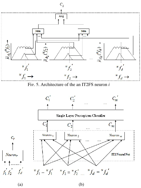
significance of the proposed simple approach is apparent for its low computational overhead and run-time performance over comparable algorithms [15-17], [53], [54] for real-time classification of brain signals. The type-2 classifier rule and inference generation using the above rule is represented in the form of a type-2 fuzzy neuron (Fig. 5), where the neuron includes d IT2FS, and for a given set of measurements
1 1,
uf uf
2 2
uf uf ,…,u u ,
d d
f f we obtain the UFSi
and LFSi to finally obtain their average Ci, representing the
degree of the measurements to fall in class i. The subscript u
above is used to designate the subject.
B. IT2FS-Based Classifier Design
The IT2FS-induced planning classifier (Fig. 3) determines four class labels including C1(braking), C2(acceleration), C3
(steering control) and C4 (no operation). The small dotted box
in Fig. 3 describes the MP classifier, comprising two modules, where the first module is an IT2FS neural net with outputs C1,
C2, C3 and C4. This neural net is realized with IT2FS neurons,
the symbol and architecture of which are given Fig. 6(a) and (b) respectively.
The next top box within the dotted small box in Fig. 3 represents the second module of the MP classifier. This module sets one of its output: Ck=1, if Ck Cl l, and sets remaining outputs to zero. In other words, if the IT2FS neural net responds with the largest output at Ckin comparison to
,
l
C l(k),then the second module sets Ck=1 andCl 0. The co-pilot, as mentioned earlier, takes binary decisions about D1 (braking), D2(acceleration) and D3(steering control) as required during driving. These decisions are considered as ground truth for the driver and consequently a failure occurs when Dk 1 but Ck =0 for anyk[1, 3].This
is given in Fig. 3 by three decision boxes. It is important to note that Dkand Ck for a given krespectively represent decision of co-pilot and decoded decision of the driver for the same planning action, say BR.
The two modules representing MP classifier here is realized by a two-layered neural net (Fig. 6(b)), where the first layer is constructed with IT2FS neurons and the second layer with perceptron neurons. Suppose, for a given instance of motor-planning by a subject s, we have d features:
1, 2, ,
s s s
d
f f f after feature selection.
Assume that the MP task has m (=4) cognitive classes, such as BR, ACC, STR control and NOP.
The principle of classification by the proposed IT2FS-NN, given in Fig. 6(b) is step-wise outlined below for an unknown subject u.
Step 1: Evaluate lower and upper firing strengths: LFSr and
r
UFS of the r-th IT2FS neuron by evaluating the t-norm (here, min) of the embedded type-1 LMFs and UMFs respectively at measurement pointsufj,j1 tod, where
( ( ))
1
j
u d
j
r LMF f
LFS Min
and ( ( ))
1
j
u d
j
r UMF f
UFS Min where, Min
d
j1
is cumulative minimum operator for varying j=1 to d.
Step 2:We next evaluate the average firing strength for the r -th neuron, given by
), (
2 1
r r
r LFS UFS
C forr1 tomclassesThis has similarity with Nie-Tan type reduction [15], [38].
Step 3: For any k,l[1,m], if Ck Cl, kl,then the response of proposed neuron k is given by
k
C=1 and Cl=0, lk.
By steps 2 and 3, we want to convey that we consider the feature sets to fall in class kif the average firing strength Ck
(using (11)) of the neuron kexceeds the same of other neurons.
Fig. 5. Architecture of the an IT2FS neuron i
(a) (b)
The perceptron learning algorithm used in Fig. 6(b) adapts the weightswk , l k=1 to m and l=1 to m by using the
learning equation:
l k l
k l
k t w t C e
w ( 1) ()
where,
wkl(t)is the weight between Ck to Clat time t,
l l
l d C
e = error signal corresponding to output
l
C with reference to pre-defined target value dl, and is the learning rate in [0,1].
C. GT2FS-Based Classifier Design
The intra- and inter-personal level uncertainty of individual sources is usually buried in the FOU of an IT2FS. In order to efficiently utilize the above forms of uncertainty, we prefer to use GT2FS-based classifier. A GT2FS, in general, is a 3-tuple given by fj, C (fj), ((fj, ) C (fj)) ,
k k
where fj is the j-th
feature, ( )
k j
C f
is the type-1 MF and ( , ( ))
k
j C j
f f
is the
secondary grade of membership of feature fj for a given
primary MF ( ).
k j
C f
In this section we propose i) one novel approach to secondary membership evaluation for a given pair of linguistic variable value and corresponding primary membership over each user supplied type-1 MF, and ii) classification of motor imageries using GT2FS-NN.
C.1 Secondary Membership Evaluation
In [55], authors proposed a novel approach for secondary MF evaluation in the settings of an optimization problem. For evaluation of secondary memberships in real-time, we here propose an alternative approach free from optimization using the following assumptions:
1.Suppose in a test, maximum marks=100 and there are 50 students, out of which a few students scored zero and 100 and the rest scored marks in [0, 100]. Now, the examiner is very certain while assigning a marks zero or 100. But he does not have the same degree of certainty while assigning a mark, say 67, to a student.
In the assignment of secondary membership, we adopted a similar policy. The secondary membership should have a maximum value equal to (or close to) 1 at the peaks and minima on the primary MF. The motivation of such selection lies in the phenomenon that the secondary grade representing the degree of primary membership should have the highest value at the peaks and minima (of the type-1 MFs) as the user is confident of assigning maximum and minimum membership values at those selected locations of the type-1 MF. Formally, we write
( fj,Ck(fj )) 1, if C~k(fj)has a local peak or minimum at fj fj.
2.The secondary membership should decrease as the linguistic variable is away from the location of the peak/minimum of the type-1 primary MF. Presuming an exponential decrease
in secondary membership at fj fl,when there exists a nearest peak/minimum at fj fj,we obtain
( l , C ( l)) ( j , C ( j)). |fj fl|
k k
f f f f e
|fj fl|
e
as ( fj,Ck(fj )) 1.
3. When a point fj[fj,fj]where fjand fjare two
nearest peak/minimum on the type-1 MF ( j),
Ck f
we obtain
the secondary MF at ( j, ( j)) Ck
f f by
| | | |
( , ( ))
[ ( , ( )). , ( , ( )). ]
j Ck j
fj fj fj fj j Ck j j Ck j
f f
Max f f e f f e
] ,
[ | | | |
fj fj fj fj
e e
Max
as ( j, ( j )) 1
Ck
f f
and ( j , ( j )) 1
Ck
f f
for fj and fjbeing peak/minimum on the type-1 MF. It may be added here that computation of secondary membership has to be performed for the primary MFs obtained from each subject. To represent the subjective primary and secondary MF for each linguistic variable, we add an extra s as the left superscript to ( j)
Ck f
and
( j, ( j)),
Ck
f f
which would look like sCk(fj)and
)) ( ,
( ~ j
C s j
s f f
k
respectively.
C.2 GT2FS-NN based Classification
In GT2FS, we need to consider subjective type-1 MF and their secondary membership values for all possible values of the linguistic variable (here, feature). To represent subjective consideration of type-1 MF, we adopt the old notations like
s j
f to describe j-th feature for subject s. Let us assume that we have n subjects to develop the complete membership space for the entire MP classifier system.
Let, Ck(sfj)be the primary MF for feature fjobtained
from experimental data of subject s for the classifier rule for class k, and ( sfj,Ck(sfj))be the secondary MF for feature
j
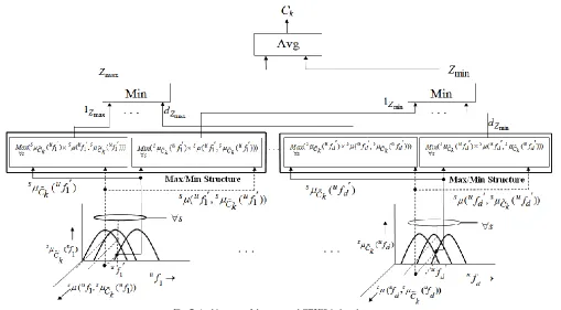
f constructed from primary MF of subject s for the classifier rule of class k. Here, we design one GT2FS-neuron to describe the k-th class classifier rule with featuresuf1,uf2, ,ufd,
where u denotes the unknown subject. The neuron produces the firing strength Ck of the k-th class classifier rule. Thus for
1. First, for each type-1 MFs (u )
j
Ck f
obtained from subject
s for featurefj, we evaluate secondary membership
( , ( ))
s u s u
j Ck j
f f
at the measurement point ufj ufj,
j=1 to d.
2.We then submit sCk(ufj)and ( , ( ))
s u u
j Ck j
f f
at the input of Max and Min blocks s,where we evaluate
max ( ( ) ( , ( )))
j s u s u s u
j j j
Ck Ck
s
z Max f f f
and
min ( ( ) ( , ( )))
j s u s u s u
j j j
Ck Ck
s
z Min f f f
for j=1 to d.
3.Now, we compute
max max 1
( )
d j j
z Min z
and min min
1
( )
d j j
z Min z
by two additional
blocks.
4. In the last step, we compute average of zmaxand zminto
compute Ck,the class membership (or firing strength) of the fired k-th classifier rule realized with the neuron. AfterCk’s are evaluated for k = 1 to m, we use a figure similar
to Fig. 6(b) with IT2FS neurons being replaced by GT2FS neurons to identify the class p where Cp=1 for Cp Cr,r and Cr 0for rp.
The GT2FS-induced classifier outperforms both the existing and the proposed IT2FS-induced classifiers because of utilization of secondary memberships in firing strength evaluation of rules. In GT2FS-induced classification, we attempted to obtain an equivalent IT2FS-like representation in the product space of primary and secondary memberships and
hence evaluated the UMF and the LMF at a given measurement point. Such product function based UMF and LMF computation improves the qualitative measure of firing strength computation, which in turn enhances the GT2FS-induced classifier performance in comparison to its IT2FS counterpart. However, the time required for secondary membership computation and processing of the product functions add extra overhead in comparison to its IT2FS counterpart. In this paper, secondary MF computation, however, is done offline.
D. Complexity Analysis
The IT2 classifier includes four main steps: i) Determining the LMF and the UMF at the given measurement points of d IT2FS present in the antecedent of a classifier rule represented by the IT2 neurons, ii) computing t-norm of the resulting LMFs (and the UMFs) obtained from d IT2FS to generate LFS and UFS respectively from each neuron, iii) Taking average of the UFS and the LFS from each neuron and iv) a forward pass in the single layer perceptron classifier to produce the desired class of the given measurement space.
The complexity of step (i) is O(d). The complexity of step (ii) is also O(d). The complexity of step (iii) is O(1). The complexity of step (iv) is O(m),where m denotes number of neurons. As we have m neurons working in parallel, their complexity represented by the first three steps, need to be considered once only. So, the overall time-complexity is 2O(d) +O(1) + O(m) O(d) +O(m). In uni-processor architecture, the complexity of the individual neurons, however, adds up, yielding an overall complexity of O(m.d) +
O(m),which approximately is O(m.d).
For GT2FS-based classifier, we need extra complexity for secondary membership evaluation plus taking product of
primary and secondary MFs at the given measurement points. The secondary membership computation is done offline. So, its complexity does not add to GT2FS classifier-overhead. Now, for d fuzzy propositions in the antecedent of the classifier rule, we need to have 2O(d) additional multiplications per neuron with respect to that in IT2FS-induced neurons. So, if the parallel architecture is fully supported, the overall complexity appears to be 2O(d)+ 2O(d) + O(m) + O(1) 4O(d) + O(m). Again, if the computation is performed on a uni-processor architecture, the computational complexity is obtained as 2m.d +2m.d + m O(m.d).
E. The KSVM Classifiers
VAFD and MEFD classifiers here are realized with KSVM, for proven performance in two class classification problems and their low computational overhead. In Fig. 2, each of the ME tasks: BR, ACC and STR control is classified into two classes, namely BR-P and BR-NP, ACC-pressed (ACC-P) and ACC-not pressed (ACC-NP) and control done and STR-control not done. The VAFD classifier classifies the obtained pre-frontal and frontal feature set into two classes: visually alert and non-alert.
A typical SVM classifier aims at designing a hyper-plane that leaves the maximum distance between the hyper-plane and the closest element from the hyper-plane (i.e., margin) from both classes. A linear support vector machine classifier can segregate linearly separable data points by an optimally chosen hyper-plane. KSVM is employed when we do not have knowledge about the linear separable nature of the data points of two classes. One approach to select the right SVM classifier is to consider KSVM with linear, polynomial and radial basis function (RBF) type kernel functions with varied parameters of the kernel and thereby determine the parameters with maximum classification accuracy. Since linear SVM is equivalent to KSVM with linear kernel function, we lose nothing by realizing the latter.
The KSVM attempts to minimize the following cost functional to find an optimal choice of the weight vector w.
1 1
( , , ) ( )
2
N T
i i i
C
Φ w w w (19) where, for i=1 to N the following constraints should hold. diw Φ xT ( i) i,
w Φ xT ( i)di i,
i 0and i 0,
In the above formulation, {(xi,di)} for i1, 2, N are the training samples with xibeing the input pattern for the
i
-th example and diis the target class label +1 or -1. Slack variable iand i represent
-insensitive loss function [48] and Φ x( i) [ 0(xi) 1( ) ( )],1
i m i
x x whose {j(xi)} for j=0 to m1denote a set of non-linear basis function. wis the m1dimensional unknown weight vector, and C is a user-defined positive parameter. Here, K( ,x xi)ΦT( ) (x Φ xi)is an inner product kernel. We here used radial basis function
kernel, given byK( ,x xi)exp( || x x i|| /22 2), polynomial kernel, given by K( ,x xi) (1 x xT i) ,d and linear kernel byK( ,x xi) (1 x xT i). We adapt C and parameter of the respective kernel function to obtain their settings for maximum classification accuracy. This is discussed in detail in the experiment section.
V. PSYCHO-PHYSIOLOGICAL EXPERIMENTS
This section provides experiments undertaken to determine certain experimental parameters concerning EEG and also to validate the principles outlined in Sections II - IV.
A. Experimental Set-up
EEG is captured from a 21-channel standalone EEG acquisition system, manufactured by Nihon Kohden with a sampling rate of 200 Hz. We also use a Logitech driving simulator for our experiment. Four EMG sensors are placed on both the hand (extensor carpi radialis longus) and the leg muscles (gastrocnemius muscles, often referred to the bulging area of the calf muscle) of the participants to test motor execution failure. The EMG data are recorded at sampling rate of 1 KHz. The detailed experimental framework is given in [47].
B. Participants
Ten subjects aged 22-30 years participated in driving experiments, among whom six are healthy (H1-H6) registered drivers, two are fatigued (F1 and F2) due to lack of sleep over last 48 hours, and the rest are driving learners (L1 and L2).
C. The Training Session
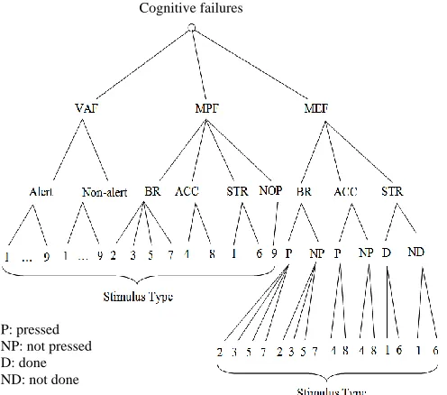
At first we prepare the training dataset. The dataset prepared for the CFD problem is presented in the form of a tree (Fig. 8). The root node of the tree denotes cognitive failures. At the next level, we present the failure types. At the third level, we list the classes under each failure type.
Fig. 8. The tree representing 43 EEG data-samples for 43 stimuli per subject per training session
P: pressed NP: not pressed D: done ND: not done
At the lowest level (leaves), we present the stimulus type for each class of the failure. The total number of stimuli/subject/training session is obtained by the count of the
leaf nodes, which here is 43. We repeat the experiment 10 times on each of the 10 subjects, thus having an EEG database of 43×10×10=4300. The length of the EEG samples collected for each stimulus is 300ms + 400ms + 400 ms= 1100ms (see Fig. 9).
C.1 Stimuli Preparation
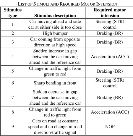
Each subject is instructed to perform driving with a given road map for 10 times, where the road-map includes nine types of visual stimuli. The list of the stimuli along the motor actions required in response to the respective stimulus is given in Table-II. The structure of the stimulus is given in Fig. 9.
TABLE-II
LIST OF STIMULI AND REQUIRED MOTOR INTENSION Stimulus
type Stimulus description
Required motor intension
1 Car moving ahead and side car at either side is too close
Steering (STR) control
2 High bumper Braking (BR)
3 Car coming from opposite
direction at high speed Braking (BR) 4
Sudden increase in gap between the car moving ahead and the reference car
Acceleration (ACC)
5 Change in traffic light from
green to red Braking (BR) 6 Sharp bending in front Steering (STR)
control 7
Sudden decrease in gap between the car moving ahead and the reference car
Braking (BR)
8 Change in traffic light from
red to green Acceleration (ACC) 9
Cars on road at constant speed and no change in road
direction/traffic signal
NOP
C.2 EEG Electrodes and Signal Acquisition
The standard 10-20 electrode placement technique has been used to locate the electrodes listed in Table-I responsible for the cognitive tasks associated with VA, MP and ME tasks. We selected pre-frontal and frontal electrodes: Fp1, Fp2, F3, F4, Fz, F7, F8 for VA detection as they are usually activated in alertness related brain-activity [56]. In addition, O1, O2 and Pz electrodes are selected for VA following [57]-[59] for possible engagement of the parietal and the occipital lobes to elicit P300 in the presence of rare/target visual stimuli.
It may be noted that usually before motor execution, the subject performs motor imagery for motor planning to mentally prepare for hand or leg movements to perform braking, acceleration and/or steering control. When there is no time-pressure, consecutive motor imagery and motor execution can be easily recognized from the parietal and the motor cortex ERD/ERS, particularly for new drivers. But when the subject is under time-pressure, the time-gap between the two ERD/ERS signals is not always visible. For hand motor imagery, the electrodes used are P3, P4, C3, C4; for hand motor execution the electrodes used are C3 and C4 while for the foot motor imagery and execution, we take the difference signals: P3 – Pz, P4 – Pz and C1 – Cz and C2 – Cz to distinguish them from the hand motor imagery/execution [60].
TABLEI
EXPERIMENTAL PROCEDURE FOR THE TRAINING SESSION
Steps Description
Step-I: Stimulus
preparation 9 stimuli as indicated in Table-II are submitted to the subject one by one, each for duration of 5 seconds after a uniform interval of 10 seconds between two successive presentations, followed by EEG acquisitions. The 9 stimuli are used to obtain four classes of subjective actions: Braking (by left foot), Acceleration (by right foot), Steering control (by both hands), and No operation/Wait for the next stimulus. The structure of an individual stimulus and timing are given in Fig. 8.
Step-II: EEG and
EMG Acquisition
i)P-300 detection from electrodes: Fp1, Fp2, F3, F4, Fz, F7, F8, O1, O2, Pz for VAF
ii) ERD/ERS detection from electrodes P3, P4, C3, C4 for MP: Steering control (hand-imagery) iii)ERD/ERS detection from electrodes C2 and Cz for
MP: Braking (left foot-imagery)
iv)ERD/ERS detection from electrodes C1, Cz, P3, Pz for MP: Acceleration (right foot-imagery)
v) ERD/ERS detection from electrodes C3 and C4 for ME: Steering control (hand-execution)
vi)ERD/ERS detection from electrodes C2 and Cz for ME: Braking (left foot-execution)
vii) ERD/ERS detection from electrodes C1 and Cz for ME: Acceleration (right foot-execution) viii) PSD detection from EMG electrodes: Ch1and
Ch2 (for hands) and Ch3 and Ch4 (for foot) to check muscle activity
Step-III: Pre-processing and Filtering
Using Elliptic filter of order 4 with pass bands i) -band (7-13 Hz) for VAF
ii) and bands (8-13, 13-30 Hz) for MPF iii) band (13-30 Hz) for MEF
Step-IV: Feature Extraction and Feature Selection
Features extracted for VAF: 11 AAR parameters Features extracted for MPF: 15 PSD + 63 DWT Features extracted for MEF: 15 PSD + 63 DWT Features selected for VAF: All extracted features Features selected for MPF and MEF: 18 out of 78 features by DE-based feature selection
Step-V: MF Construction
IT2FS Construction
1. Type-1 MF construction for each feature from multiple trials of the same of the same subject 2. Construction of Mixture of Gaussians by repeating experiments on 10 subjects
3. Taking max and min of the Gaussians to obtain UMF and LMF of IT2FS
GT2FS Construction
1.For each Gaussian primary MF obtained in step-2 above, compute secondary MFs at the desired value of linguistic variable x and primary MF: A( ).x
Step-VI: Classifier Training
1. Define class labels for IT2FS/GT2FS classifiers 2. Feed extracted features to the classifier:
(IT2FS/GT2FS) and measure error at the output of layer 2 neurons
3. Adjust the weights of the second layered neurons by Perceptron Learning algorithm.
C.3 Pre-processing and Filtering
We here select Infinite Impulse Response (IIR) filters over Finite Impulse Response (FIR) filters because of its requirement of fewer filter coefficients with respect to the latter for a given order of the filter.
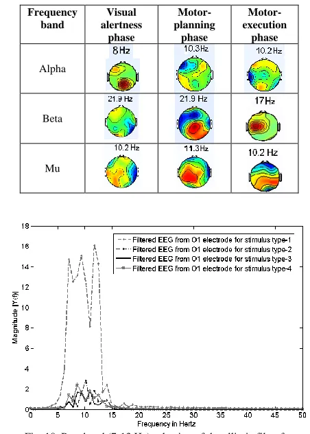
For realization, we select Elliptic filter of order 4 over Butterworth, Chebyshev-I and Chebyshev-II filters for its sharper roll-off around the cut-off frequencies than the rest. For pass band selection of the elliptic filters, we obtain the centre-frequency of the bands and scalp maps for three cognitive tasks, as given in Table III.
The filtered signals in the pass band of the VA and motor imagery classes from occipital and motor cortex regions respectively are given in Fig. 10 and 11. It is confirmed from both the figures that alpha band (8-13 Hz) is associated during visual alertness and beta (13-30 Hz) band is active during motor execution tasks.
TABLE III
ACTIVATION OF SCALP MAPS FOR DIFFERENT COGNITIVE MODALITIES AT DIFFERENT FREQUENCY BANDS
For each driving session, we take ICA of the 19 electrodes and observe that for the independent components 1, 3, 4, 5, 6, 7, 8, 9, 14, 16, 17, we have circular (enclosed) red regions indicating activation of the corresponding brain regions (Fig. 12). The remaining components are ignored since these are activated due to eye-blinking and muscle artifacts.
C.4 EEG Feature Selection
To select features for a given cognitive task, we plot the feature values against feature-count, and note the discriminating features for the sub-classes (say, BR, ACC, STR and NOP) of the cognitive task (say, MP/ME). We extract AAR parameters for VAFD, and PSDs and DWT coefficients for MPFD and MEFD. To obtain feature sets, the signal is first segmented using a moving window with window size = 500ms, which yields a data array of 10 samples/window at 200 Hz sampling rate.
Fig. 11. Pass band (13-30 Hz) selection of the elliptic filter during execution of four motor actions for four stimuli
Fig. 10. Pass band (7-13 Hz) selection of the elliptic filter for occipital EEG for four stimuli
Fig. 12. ICA scalp components from 19 EEG electrodes. Here, red color denotes the highest activation, whereas, blue color represents the lowest
activation.
Frequency band
Visual alertness
phase
Motor-planning
phase
Motor-execution
phase
Alpha
Beta
Mu
During feature extraction, this sliding window is moved from left-to-right along with each EEG data array and the features: AAR, PSD and DWT coefficients are computed to obtain the required features for VAFD, MPFD and MEFD respectively. Fig. 13 shows PSD feature discrimination during MPFD. Feature discrimination plots for AAR and DWT parameters are given in [47].
After feature extraction, we finally obtain 11 AAR, 15 PSD and 63 DWT features. For (15 + 63) = 78 dimensional MPF and MEF feature sets, we require to execute the evolutionary feature selection to select fewer features (here 18) without losing their inherent power of inter-class separation. The superiority of the proposed DE-based feature selection strategy against the traditional principal component analysis (PCA) is validated using confusion matrices (See [47]).
The rest of the steps in Table-I, including MF construction and classifier training are self-explanatory. The classifier performance in the training phase is not given here for space restriction (See [47] for details). Only the parameter selection of KSVM with linear, polynomial and RBF Kernels are given in Tables. It is observed from the Table IV that the KSVM with RBF Kernel yields the best classification accuracy in the training phase with C= 1 and =0.75 (marked in bold). The polynomial kernel (with d=2, 3) based KSVM however yields worse classification accuracy than the RBF kernel and the linear kernel (d=1) based KSVM (Table V).
TABLE IV
CLASSIFICATION ACCURACY OF KSVM-RBFCLASSIFIER FOR VARIED C and
C
0.01 0.75 1.00 100
0.5 71.44 83.55 80.22 77.33 1 77.22 95.22 88.44 81.55 10 66.55 78.11 73.33 69.11
TABLE V
CLASSIFICATION ACCURACY OF KSVM-LINEAR AND POLYNOMIAL CLASSIFIER FOR
VARIED C AND d
C d
1 2 3
0.5 91.33 89.11 87.22 1 95.00 93.11 90.00 10 88.55 86.33 81.33
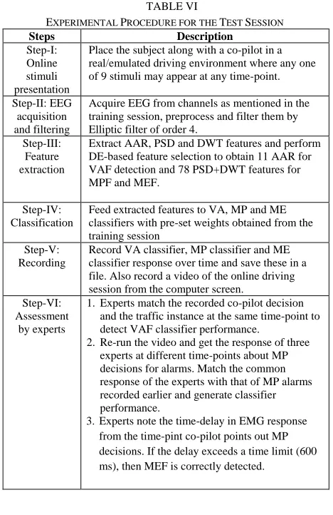
D. The Test Session
Table- VI provides a summary of the main steps undertaken in the test phase. Steps-I to III are similar with those in the training session with the following exception. Although for both the training and the test sessions we used the same driving simulator, the training was performed with presentation of individual stimulus one by one in a discrete sense. However, the test session is performed in a continuous mode. So, any stimulus might appear at any time-point. After the assessment of the classifiers by a team of experts as indicated in Table-VI, we analyze the classifier performance as given in the next section.
VI. PERFORMANCE ANALYSIS
This section provides experimental basis for performance analysis and comparison of the proposed classifiers with traditional/existing ones. It also undertakes experiments for lead-time estimation and objective performance of the proposed CFD system with respect to different stimuli, representative of traffic conditions.
A. Performance Analysis of VAFD classifier
Here, we compare the run-time and relative classification accuracy of LDA and KSVM with linear, polynomial and RBF kernels, when experimented over 10 subjects, each experiencing 4 BR, 2 ACC and 2 STR control instances (See Fig. 8) for 10 times, and thus yielding altogether 400 BR, 200
TABLE VI
EXPERIMENTAL PROCEDURE FOR THE TEST SESSION
Steps Description
Step-I: Online stimuli presentation
Place the subject along with a co-pilot in a real/emulated driving environment where any one of 9 stimuli may appear at any time-point. Step-II: EEG
acquisition and filtering
Acquire EEG from channels as mentioned in the training session, preprocess and filter them by Elliptic filter of order 4.
Step-III: Feature extraction
Extract AAR, PSD and DWT features and perform DE-based feature selection to obtain 11 AAR for VAF detection and 78 PSD+DWT features for MPF and MEF.
Step-IV: Classification
Feed extracted features to VA, MP and ME classifiers with pre-set weights obtained from the training session
Step-V: Recording
Record VA classifier, MP classifier and ME classifier response over time and save these in a file. Also record a video of the online driving session from the computer screen.
Step-VI: Assessment
by experts
1.Experts match the recorded co-pilot decision and the traffic instance at the same time-point to detect VAF classifier performance.
2.Re-run the video and get the response of three experts at different time-points about MP decisions for alarms. Match the common response of the experts with that of MP alarms recorded earlier and generate classifier performance.
3.Experts note the time-delay in EMG response from the time-pint co-pilot points out MP decisions. If the delay exceeds a time limit (600 ms), then MEF is correctly detected.