Article
Real-time Analysis of a Modified State Observer for
Sensorless Induction Motor Drive used in Electric
Vehicle Applications
Mohan Krishna S 1, Febin Daya J.L 1, Sanjeevikumar P 2,*, and Lucian Mihet-Popa 3
1 School of Electrical Engineering, VIT University - Chennai Campus, Chennai 600 048, India; [email protected]; [email protected]
2 Department of Electrical and Electronics Engineering Science, University of Johannesburg, Auckland Park, Johannesburg 2006, South Africa
3 Faculty of Engineering, Østfold University College, Kobberslagerstredet 5, 1671 Kråkeroy; Building: S 316, Norway ; [email protected]
* Correspondence: [email protected]; Tel.: +27-79-219-9845
Abstract: The purpose of this work is to present an adaptive sliding mode luenberger state observer with improved disturbance rejection capability and better tracking performance under dynamic conditions. The sliding hyperplane is altered by incorporating the estimated disturbance torque with the stator currents. Also, the effects of parameter detuning on the speed convergence is observed and compared with the conventional disturbance rejection mechanism. The entire drive system is first built in simulink environment. Then, the simulink model is integrated with RT-Lab blocksets and implemented in a relatively new real-time environment using OP4500 real-time simulator. Real-time simulation and testing platforms have succeeded offline simulation and testing tools due to their reduced development time. The real-time results validate the improvement in the proposed state observer and also correspond to the performance of the actual physical model.
Keywords: state estimation; model reference; sliding mode; real-time; parameter detuning
1. Introduction
The utility of induction motors has risen considerably owing to its integration with power electronic converters, which made variable frequency operation realizable. This, in turn, made the induction motor the workhorse of the industry. Of all the variable frequency control strategies, the vector control or field oriented control principle was the most popular. It provided independent control of torque and flux resulting in fast torque response. The field orientation can be achieved by directly measuring the magnitude and direction of the flux by means of flux sensors or hall effect sensors in the machine (Direct Vector control) or it can be imposed indirectly by a slip frequency component from the rotor dynamics (Indirect Vector control). The latter was more feasible as it did not require the use of additional flux sensors which would occupy additional space and cost. The indirect vector control principle is shown in the phasor diagram expressed as steady state dc quantities in Figure 1.
By decoupling the induction motor at synchronously rotating reference frame, and forcing the direct axis stator current component (field producing) in phase with the rotor flux and orthogonal to the quadrature axis stator current` component (torque producing), independent control of torque and flux is obtained. However, the indirect vector control implementation required the utility of a shaft speed encoder to sense the rotor speed, which was processed along with the speed command to generate the reference torque request for vector control. The presence of the shaft speed encoder implies additional electronics, cost and mounting space. Therefore, to eliminate the shaft speed encoder, the speed estimation techniques were used.
Figure 1. Indirect vector control principle.
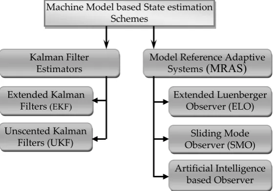
The speed was estimated from either the terminal quantities of the machine or from its rotor saliency. However, speed estimation from the machine model was easier to implement, occupied less computational space and were most effective. Considerable research over the past two decades focused primarily on sensorless control of induction motor [1], with special emphasis on estimation from the machine model [2]. The state estimation schemes are shown in Figure 2.
During the earlier stages, Extended Kalman Filter (EKF) based estimators [3-5] were widely used for speed estimation, but they give accurate results only if the system dynamics are linearized and had an inherent disadvantage of a high sampling frequency and were computationally expensive. Estimators based on Model Reference Adaptive Systems (MRAS), Extended Luenberger Observers (ELO) and Sliding Mode Observers (SMO) [6-7] had a wider utility and were more extensively used owing to ease of use and flexibility. Besides, several configurations varying from lower order to higher order observers, as well as integration of variable structure or artificial intelligence could be developed from the MRAS. All the model based schemes were sensitive to variations or incorrect settings of parameters.
Figure 2. Machine model based state estimation schemes.
The MRAS and ELO were mainly used for simultaneous state estimation in order to prevent a mismatch between the actual and estimated values of the parameters under all speed ranges. Several
α
=a
β
q
d
θ
Machine Model based State estimation Schemes
Model Reference Adaptive
Systems
(MRAS)
Artificial Intelligence based Observer
Sliding Mode Observer (SMO) Extended Luenberger
Observer (ELO) Kalman Filter
Estimators
Unscented Kalman Filters (UKF) Extended Kalman
studies focused on the performance analysis and parameter estimation [8-10] for the drive at low and zero speed regions [11-13].As stated before, variable structure or sliding mode observers (SMO) based on MRAS have been implemented for wide speed bandwidth estimation and faster parameter convergence by constraining the states of the system to the sliding hyperplane [14-17]. [18] implements a Luenberger-SMO which estimates the critical parameters online. It is demonstrated by means of Hardware in the loop (HIL) simulation setup with an FPGA based controller and an induction motor, to verify the robustness of the algorithm. [19] presents a Sliding Mode-MRAS observer based on a super twisting algorithm (STA), where, the variations in critical parameters are intentionally considered. In the standard configuration of MRAS, the reference model is replaced by a stator current observer which is designed based on STA. This, in turn, is insensitive to rotor resistance variations and disturbances when the states converge on the sliding hyperplane. The chattering phenomenon is eliminated and near zero speed operation is realized by means of a parallel identification of stator resistance. In [20], the concept of adaptive luenberger flux observation is applied for the state estimation of a sensorless symmetrical six phase induction machine subjected to unbalanced operation. In addition to it, the efficacy and performance of the observer is tested by incorporating mechanical and electrical disturbances during the normal operation of the machine. Variation of the inertia up to the maximum value and the loss of one or more stator phases are considered for all the test cases of unbalanced conditions. There are also certain class of load torque rejection observers which have been implemented. These disturbance observers, either comprise of a mechanical model of the motor or have error components which are dependent on the rotor speed, or gain coefficients dependent on the stator frequency [21-24]. In [24], the decoupling of current and subsequent control of the current components is applied to induction motor by employing a sliding mode controller and a disturbance observer. The coupled terms are modeled as disturbance, which, after observation are utilized in the control law. Also, the rotor speed is estimated based on the magnetizing current and the lyapunov stability criterion is used to ensure closed loop stability. Several of the above categories of observers have been implemented in many experimental platforms and also been verified by means of HIL testing.
The purpose of this paper is to demonstrate the improvement in the rejection of the external load by the proposed observer. The sliding hyperplane is altered and the disturbance estimated from the mechanical model is integrated into the sliding hyperplane along with the real and estimated stator currents [17]. The observer, along with the drive system, is first built using Matlab/Simulink blocksets and then validated in a comparatively new real time simulation platform, RT-Lab, developed by Opal-RT and the real-time results add more credibility as compared to any other offline simulation platform.
2. General Configuration of MRAS and System Modeling
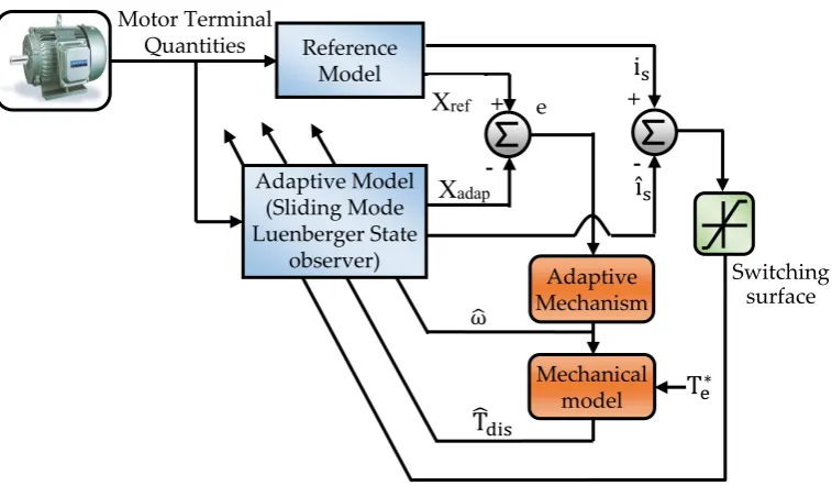
Adaptive control is mainly used for parameter adaptation. The essence of an adaptive control mechanism is to adapt to the controlled system with parameters which need to be estimated. The concept of parameter adaptive MRAS along with the parallel disturbance torque estimation mechanism is illustrated in Figure. 3. There is a reference motor model and the adaptive model as a function of the parameter to be estimated. The adaptive mechanism is used to ensure that the state of the observer (process) converges to the state of the motor (plant). Therefore, we have an optimization criterion X and the error to be constrained:
X = e dt (1)
e = X − X (2)
Figure 3. Basic configuration of parameter adaptive MRAS scheme with parallel disturbance torque estimation.
2.1. Structure of Sliding Mode Luenberger State observer
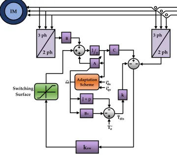
The reduced order Sliding mode Luenberger observer (SMLO) with the modified switching surface is shown in Figure. 4. where, ‘A’ is the parameter matrix, ‘^’ is used for estimated parameters, ‘X’ is the state variables comprising of the d and q axes stator currents and rotor fluxes, ‘ksw’ is the reduced order observer switching gain matrix, chosen in such a way that the eigen values of the observer and the machine are maintained proportional to ensure stability under normal operating conditions. ‘J’ is the moment of inertia, ‘p’ is the differential operator, ‘BV’ is the viscous friction coefficient, ‘T∗’ and ‘T ’ is the reference model electromagnetic torque and the estimated disturbance torque, ‘k’ is an arbitrary positive gain [17]. The purpose of a sliding mode or variable structure strategy is to modify the dynamics of a non linear system state by means of a high frequency switching surface or a sliding hyperplane. The sliding hyperplane is selected in such a way that the Lyapunov function candidate ‘V ‘utilized for obtaining the convergence mechanism, and its derivative satisfies the Lyapunov stability criterion [17, 25]. V’ is a scalar function of the sliding hyperplane ‘S’. Therefore,
V(S) = S(x)S(x) (3)
The control law is:
u(t) = u (t) + u (t)
(4)
Where, u(t), ueq(t) and usw(t) represent the control, equivalent control and the switching vector. For
stability, the switching vector is obtained [17, 26]:
u (t) =sign(S(x, t)) (5)
Where, sign(S) =
−1 for S < 0 0 for S = 0 +1 for S > 0
-η is the switching control gain chosen such that (3) is negative definite, implying S(x)S(x) < 0 thereby constraining the effect of the external disturbance. But, the high frequency switching plane
Figure 4. Proposed state observer with the modified switching hyperplane
increases non linearity of the observer, leading to chattering. Therefore, to eliminate the effect of this
unwanted phenomenon, a saturation function having boundary layer of width (Φ) is used by
replacing sign(S) with sat(S/Φ) and is given by [17]:
sat(S/) = sign if () 1
if () < 1
(6)
Based on the theory of MRAS, the following equations depict the structure of the proposed observer scheme with the conventional and modified sliding hyperplane. The reference and the adaptive model are represented in state space form as they aid in the formulation of control and estimation problems [17, 27].
2.1.1. Reference Model (Motor)
= [A]x + [B]u (7)
y = [C]x (8)
Where,
x = i , i , ψ , ψ , A = AA AA ,
B = [ I 0] , C = [I, 0], u = [ v v ]
Switching Surface
J ∗ p
∗ BV
B
1 C
IM
k
k
sw3 ph
2 ph
3 ph
2 ph
Adaptation Scheme
I = 1 00 1, J = 0 −11 0 ,
A = − R σL +
1 − σ
σT I = a I,
A = I − ω J = a I + a J,
A = I = a I,
A =−1
T I + ω J = a I + a J
2.1.2
.
Estimation of Disturbance Torque from the mechanical modelBy exploiting the machine model, the disturbance torque is estimated by utilizing the reference model electromagnetic torque and the estimated speed respectively.
T = T∗− J − B ω (9)
2.1.3. SMLO 1 – Observer with conventional disturbance rejection mechanism (Adaptive model)
= A x + [B]u + k sat( ı̂ − i ) + d (10)
Where, the sliding hyperplane,
s = ı̂ − i and d = kT and
y = [C]x (11)
Where, ı̂ , i = estimated and measured value of stator current
A = A A A A ,
A = I − ω J = a I + a J,
A =−1
T I + ω J = a I + a J
The switching gain ‘ksw’ is designed by the following lower order matrix given by,
k = −kk kk (12)
The switching gain matrix is designed appropriately to make (4) stable by means of pole placement. The eigen values are designed in such a way that, for the observer, they are comparatively more negative to that of the motor so that they ensuring faster convergence of the desired performance to the process. Therefore,
k = (m − 1)a (13)
k = k , k ≥ −1 (14)
2.1.4. SMLO 2 – Observer with modified disturbance rejection mechanism (Adaptive model)
The state dynamic equation is altered by changing the sliding hyperplane i.e., by including the estimated disturbance torque [17].
= A x + [B]u + k sat ı̂ − i − d (15) Therefore, the sliding hyperplane becomes,
s = ı̂ − i − d and d = kT and
y = [C]x (16)
2.1.5. Adaptive Mechanism
The Lyapunov function candidate used for speed derivation mechanism and to ensure stability is given by:
V = e e +( ) (17) Where, λ is a positive constant.
We have:
= e [(A + GC) + (A + GC)]e − + (18)
Where, e = i − ı̂ , e = i − ı̂
The second and third term of (18) is equalized to realize the expression for the estimated speed given by:
= (e φ − e φ ) (19)
‘c’ being an arbitrary positive constant. The difference between SMLO2 and SMLO1 is the way in which the estimated disturbance is added and constrained in the sliding hyperplane along with the stator current error. The complexity of the observer increases due to the presence of the speed adaptation loop, the disturbance estimation and adaptation loop and the Luenberger observer gain loop, however, by tuning the feedback and switching gains, the dynamic performance and the stability of both the observers can be improved.
2.2.Structure of Current regulated Vector controller
Current regulation or tolerance band current control has a fast torque response and is independent of load parameters. The speed error is processed by a PI controller whose output is the reference torque.
e = ω − ω∗ (20)
T∗= e k + (k /s) ∗ T (21) Where, ec is the speed error, kp and ki are the proportional and integral gains for tuning the speed error, Ts is the sampling time. For operation in the motoring and flux weakening region, the rotor flux is constant for the former and as a function of the speed for the latter.
ψ = 0.96,If ω < ω (22)
The orthogonal direct and quadrature axes stator current components are [1]:
i ∗= 1 + (24)
i ∗= (25) As the slip speed is used for imposing the field orientation, the field angle is determined from the slip speed, therefore:
θ = θ + θ (26) The three phase reference currents are obtained from the decoupled reference components of current by means of inverse transformation given as follows:
i∗ = i sinθ + i cosθ (27)
i∗ = −i cosθ + ⎷3 i sinθ + i sinθ + ⎷3i cosθ (28)
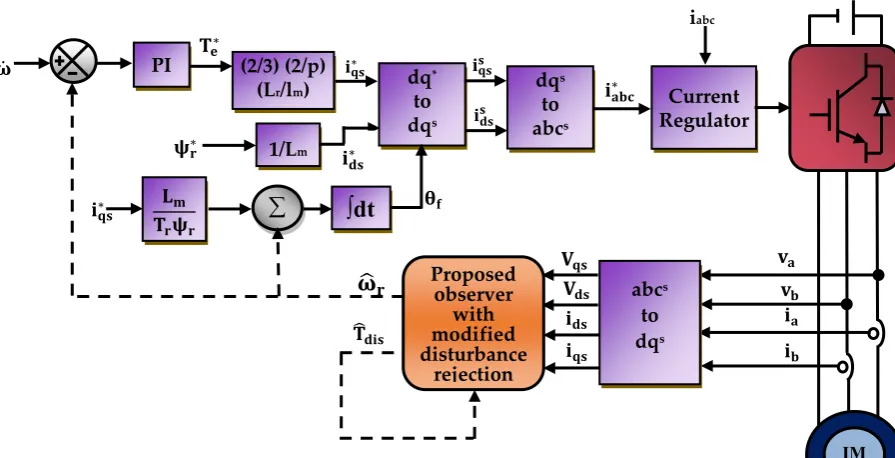
i∗ = −(i∗ + i∗ ) (29) The three phase reference current components are compared with the actual sensed three phase currents by means of hysteresis regulation and the gating pulses for the (VSI) are generated. The hysteresis band is selected keeping the current and subsequent torque pulsation in mind. The entire sensorless drive scheme is illustrated in Figure 5 [17].
3. The Concept of Real-Time Simulation and RT Lab
Real-time simulation and test platform is one in which the computer model’s performance corresponds to the performance of the actual physical system [28-30]. It would take the same amount of time like any real world application. Unlike many offline simulation platforms, where a variable step solver is used, in real-time, a fixed step discrete solver is used. For a given computer model, in a real-time simulation, the processing of inputs, model calculations and the processing of outputs, should be less than the fixed step. If it exceeds the fixed step, a phenomenon known as over run would occur. Therefore, it is imperative that the real-time simulator should produce the model calculations and output within the same time interval corresponding to its actual physical counterpart. The applications ranges from mechatronics, power electronic and power system based concepts to gaming and process control.
Figure 5. VSI fed speed sensorless induction motor drive system
Vdc IM Proposed observer with modified disturbance rejection PI (2/3) (2/p)
(Lr/lm)
There are various real time simulators available such as xPC Target, for power electronic system simulation there is eFPGAsim and eDRIVEsim and for power system simulation, we have HYPERSIM and RTDS.
RT-Lab is a distributed real- time platform with features ranging from virtual, control and plant prototyping, model based design etc. It is flexible and has a fast execution time and also, can be utilized for real-time Processor-in-Loop (PIL) and hardware in the loop (HIL) applications. The package is compatible with various offline platforms such as Matlab/Simulink, Labview etc. The mathematical and dynamic model of the drive system is built in Simulink environment using sim-power systems toolbox. This acts as the front end interface after which the model is integrated with RT-Lab blocksets. RT-Lab generates the code to be simulated in a single or multiple targets. Here, the real-time simulation target used is OP4500 developed by Opal-RT. It is a multi core target where the plant and controller can be placed in different cores.
It comprises of analog and digital I/O channels with signal conditioning and is also integrated with powerful XILINX Kintex 7 FPGA which has a very high processing power.
4. Real-Time Simulation Results
The sensorless drive system is modeled and built offline using sim power systems toolbox in Simulink in the workstation. The offline simulink model uses a variable step solver. The RT-Lab integrated real-time platform uses a discretised fixed step time solver with a step size of 50 μs. The workstation is connected to the OP4500 real-time simulator through TCP/IP protocol. The target executes the model and the results are viewed and recorded in the workstation which is the front end interface. The model is executed and analyzed dynamically for different test cases as presented below:
4.1. Performance at flux weakening
Figure 6. (a) Estimated speed of SMLO 1 (b) zoomed version of (a) (a)
Figure 7. Estimated Disturbance torque of SMLO1
Figure 8. Electromagnetic Torque of SMLO1
Figure 10. (a) Estimated speed of SMLO 2 (b) zoomed version of (a)
Figure 11. Estimated Disturbance torque of SMLO2
Figure 12. Electromagnetic Torque of SMLO2 (a)
Figure 13. Estimated Rotor flux of SMLO2
4.2. Performance at step speed command
Figure 14. (a) Estimated speed of SMLO 1 (b) zoomed version of (a) (a)
Figure 15. (a) Estimated speed of SMLO 2 (b) zoomed version of (a)
Figure 16. Estimated disturbance torque of (a) SMLO 1 (b) SMLO 2 (a)
(b)
(a)
Figure 17. Estimated Rotor flux of (a) SMLO 1 (b) SMLO 2
4.3. Performance at Low speeds
Figure 18. (a) Estimated speed of SMLO 2 (b) zoomed version of (a) (a)
(b)
(a)
Figure 19. Estimated Disturbance torque of SMLO2
4.4 Effect of parameter detuning on the dynamic performance
Figure 20. Speed tuning signal for 50% incorrect setting of Stator resistance (Rs) and rotor time constant (Tr) for (a) SMLO1 (b) SMLO2
(a)
Figure 21. Speed tuning signal for nominal setting of Stator resistance (Rs) and rotor time constant (Tr) for (a) SMLO1 (b) SMLO2
Figure 22. Speed tuning signal for 150% incorrect setting of Stator resistance (Rs) and rotor time constant (Tr) for (a) SMLO1 (b) SMLO2
(a)
(b)
(a)
4.5 Switching surface and convergence of the stator current error
Figure 23. SMLO 1 (a) Sliding surface (b) Flux component of stator current (c) Torque component of stator current (d) Stator current error
(a)
(b)
(c)
Fig. 25. SMLO 2 (a) Sliding surface (b) Flux component of stator current (c) Torque component of stator current (d) Stator current error
5. Analysis and Discussion
The motor parameters and ratings used for the real-time simulation are given in appendix. In order to emphasize on the improvement in the performance of SMLO2 over SMLO1, some results are magnified to present a clearer picture. Parameter estimation of an observer at flux weakening regions is significant as it indicates its robustness for a wider speed bandwidth as also, its tracking performance at constant power region. Here, the observers are tested at low flux weakening region
(a)
(b)
(c)
for a given speed command of 165 rad/s. Although, both reach the reference speed at almost identical time, the estimated speed oscillations are comparatively very high for SMLO1 as shown in Fig. 6(a) as compared to SMLO2 shown in Fig. 10(a). In the zoomed version shown in Fig. 6(b), the oscillation is as high as 70 rad/s for the speed command of 165 rad/s which is almost 42%, whereas for SMLO2 in Fig.10(b), although there is an initial overshoot and undershoot, the oscillation is initially around 20 rad/s, which is around 12% and gradually dies out after 6 seconds. Once again, the estimated disturbance torque of SMLO 2 in Fig. 11 has relatively lesser ripples as compared to SMLO1 in Fig. 9. These can be attributed to lesser current pulsation and better disturbance rejection capability of SMLO2, as both, the stator error convergence and the estimated disturbance torque are constrained within the sliding surface. The electromagnetic torque in Fig. 8 and Fig. 12 for both the observers almost follows the profile of the disturbance torque, since the viscous friction coefficient and the inertia constant are of a low value. The estimated rotor flux of SMLO1 in Fig. 9 has relatively more oscillations and the magnitude is increasing with time as compared to the estimated rotor flux of SMLO2 in Fig. 13. This shows that the SMLO2 has better reception to flux weakening and operates well in this region. The difference is seen more distinctly at step speed command (initially 50 rad/s, after 2 seconds, stepped upto 150 rad/s, after 7 seconds, stepped down to 100 rad/s) which covers a wide speed bandwidth. SMLO1 initially, tracks well for both 50 rad/s and 150 rad/s, but, during deceleration from 150 rad/s to 100 rad/s, there is a very high spike in the estimated speed (of almost 100 rad/s) shown in Fig. 14(a), which could prove detrimental to the drive system. This is mainly due to the sudden change in the flux level of the motor and SMLO1, which directly affects its speed convergence. Even after settling down at 100 rad/s, after about 10 seconds, oscillations persist ranging between 98.5 – 101 rad/s, shown in Fig. 14(b). SMLO2 in comparison tracks more smoothly and accurately, even during deceleration as shown in Fig. 15(a). The oscillations in the estimated speed are greatly reduced as shown in Fig. 15(b), ranging almost between 99.9 – 100.1 rad/s, which proves it’s near accurate and superior tracking as compared to SMLO1. Even the estimated disturbance torque profile of SMLO2 shown in Fig. 16(b) is comparatively smoother with lesser pulsations as compared to SMLO1 shown in Fig. 16(a). The estimated rotor flux performance for SMLO1 and SMLO2 can be observed in Fig. 17(a) and Fig. 17(b). Here again, the latter gives smoother flux performance in spite of variations in the commanded speed at different time intervals, resulting in better torque holding capability.
error, as both are dependent on each other. However, as compared to SMLO1, shown in Fig. 23(a) and Fig. 23(d), both, the stator current error and the sliding surface of SMLO2 are slightly displaced in the negative range, shown in Fig. 24(a) and Fig. 24(d). This can be primarily due to change in the configuration of the sliding surface, as, along with the stator current error, it also has to constrain the effect of the estimated disturbance torque. The direct and quadrature axes stator currents are also obtained, as shown in Fig. 23(b) and Fig. 23(c) for SMLO1 and Fig. 24(b) and Fig. 24(c) for SMLO2. Although both are similar, the presence of pulsations in the stator current components, both, during steady state and transient conditions give rise to subsequent torque and flux pulsations in the observers. Also, due to high power rating of the motor, the stator current dynamics play a major role in the torque performance. However, it is seen that the SMLO2 comparatively displays better dynamic and steady state performance due to its ability to contain the stator current dynamics and ensure that it does not affect the tracking. For the entire study, the load torque was maintained constant at 100 Nm. For the last two test cases, along with the constant load torque, the speed command was also maintained constant at 100 rad/s respectively. Since hysteresis band current regulation is used, the exact switching frequency cannot be predicted, however, the maximum switching frequency which is realizable by the OP45OO target is (1/(2*time step)) which is 10 kHz. As the model has been successfully executed by the target, it can be safely concluded that the equivalent switching frequency is within 10 kHz. The entire testing and analysis was performed in the motoring mode at low, medium speeds and low flux weakening regions. The Table 1summarizes the observations from the above analysis for both the observers.
Table 1. Salient features of both the observers
Test cases SMLO 1 SMLO 2
Low flux weakening region
Maximum Speed oscillation of around 70 rad/s (around 42% of the reference value). Speed Oscillations
do not die out.
Initial maximum speed oscillation of around 20 rad/s (around 12% of the reference value). Speed Oscillations gradually reduce with time.
Step speed command
Very high overshoot and undershoot observed at the instance of fast
deceleration.
Smoother tracking during fast acceleration and deceleration.
Low speed operation
Does not track, becomes unstable and speed convergence goes out of
bounds.
Tracks well, initial undershoot and overshoot which results for a
very small interval of time.
Disturbance Torque Higher torque pulsations as a result of high stator current pulsation.
Comparatively lower torque pulsation resulting in better
torque holding capability. Speed and Stator
error convergence
Slower convergence, higher speed and stator current error
Faster convergence, resulting in smoother tracking
6. Conclusions
Acknowledgments: No funding resources
Author Contributions: Mohan Krishna, Febin Daya, Sanjeevikumar Padmanaban, as developed the proposed ac drives research work and implemented with numerical simulation software and hardware implementation using RT-Lab solutions. Further, Sanjeevikumar Padmanaban, Lucian Mihet-Popa extended the insight, technical expertise to make the work quality in its production. All authors involved in validating the numerical simulation results with hardware implementation, experimental test results in accordance with developed theoretical background. All authors involved and contributed in each part of the article for its final depiction as research paper”.
Conflicts of Interest: The authors declare no conflict of interest.
Appendix A
The ratings of the model considered for the study are: A 50 HP, 415 V,3Φ, 50 Hz, star connected, four-pole induction motor with equivalent parameters: Rs = 0.087 Ω, Rr = 0.228 Ω, Lls = Llr = 0.8 mH, Lm = 34.7 mH, Inertia, J = 1.662 kgm2, friction factor = 0.1.
Nomenclature
The symbols and notations used are given below:
idss, iqss,idrr,iqrr - direct and quadrature axes stator and rotor current components in stationary and rotating frame vdss,vqss - direct and quadrature stator voltages in stationary frame
Tr , Rs, Rr - Rotor time constant, Stator and Rotor resistance
σ, Lr, Lm, Ls - Leakage reactance, Rotor, Magnetizing and Stator self Inductance Lls, Llr - Stator and Rotor Leakage Inductances
ω,ω,ω∗,ω - Actual, estimated, reference and base synchronous speed
ψdss, ψqss, ψdrs,ψqrs - direct and quadrature axes stator and rotor flux linkages in stationary frame
φ ,φ - direct and quadrature axes estimated rotor flux linkages θ,θ ,θ , T∗ - field, slip and rotor angles and Torque reference
i ∗, i∗
- direct and quadrature axes stator currents in synchronously rotating frame
i∗, i∗ , i∗ - Three phase reference currents
References
1. Anitha, P.; Badrul, H.C. Sensorless control of inverter-fed induction motor drives. Electr. Pow. Syst. Research 2007, 77, pp. 619-629.
2. Zhiping, Y,; Qiuqin, Y,; Yong, Y. Induction Motor Speed Control Based on Model Reference. Procedia Engineering 2012, 29, pp. 2376-2381.
3. Abd El-Halim, A.F.; Abdulla, M.M.; El-Arabawy, I.F. Simulation Aides in Comparison between Different Methodology of Field Oriented Control of Induction Motor Based on Flux and Speed Estimation. Proceedings of the 22nd International Conference on Computer Theory and Applications, Alexandria, Egypt, 13-15 Oct 2012.
4. Danan, S.; Wenli, L.; Lijun, D.; Zhigang, L. Speed Sensorless Induction Motor Drive Based on EKF and Γ-1 Model. Proceedings of IEEE International Conference on Computer Distributed Control and Intelligent Environmental Monitoring, Changsha, China, 19-20 Feb 2011.
5. Alonge, F.; D’Ippolito, F.; Sferlazza, A. Sensorless Control of Induction-Motor Drive Based on Robust Kalman Filter and Adaptive Speed Estimation. IEEE Trans. Ind. Electron 2014, 61, pp. 1444-1453.
6. Rezgui, S.E.; Benalla, H.; MRAS sensorless based control of IM combining sliding-mode, SVPWM, and Luenberger observer. Proceedings of International Conference on Computer as a Tool, Lisbon, Portugal, 2011.
7. Zheng, Y,; Loparo, K.A. Adaptive Flux Observer for Induction Motors. Proceedings of American Control Conference, Philadelphia, USA, 1998.
8. Ticlea, A.; Besancon, G. Observer Scheme for State and Parameter Estimation in Asynchronous Motors with Application to Speed Control. Eur. J. Control 2006, 12, pp. 400-412.
10. Levi, E.; Wang, M. Impact of Parameter Variations on Speed Estimation in Sensorless Rotor Flux Oriented Induction Machines. Proceedings of IEEE Power Electronics and Variable Speed Drives, London, UK, 21-23 Sep 1998.
11. Gadoue, S.M.; Giaouris, D.; Finch, J.W. Performance Evaluation of a Sensorless Induction Motor Drive at Very Low and Zero Speed Using a MRAS Speed Observer. Proceedings of IEEE 2008 Region 10 Colloquium and the Third International Conference on Industrial and Information Systems, Kharagpur, India, 2008.
12. Rashed, M.; Stronach, A.F. A stable back-EMF MRAS-based sensorless low-speed induction motor drive insensitive to stator resistance variation. IEE Proc. E Trans. Electr. Power. Appl. 2004, 151, pp. 685-693. 13. Beguenane, B.; Ouhrouche, M.A.; Trzynadlowski, A.M. A new scheme for sensorless induction motor
control drives operating in low speed region. Math. Comput. Simulation 2006, 71, pp. 109-120.
14. Lascu, C.; Boldea, I.; Blaabjerg, F. A Class of Speed-Sensorless Sliding-Mode Observers for High-Performance Induction Motor Drives. IEEE Trans. Ind. Electron. 2009, 56, pp. 3394-3403.
15. Gadoue, S.M.; Giaouris, D.; Finch, J.W. MRAS Sensorless Vector Control of an Induction Motor Using New Sliding-Mode and Fuzzy-Logic Adaptation Mechanisms. IEEE Trans. Energy. Convers.2010, 25, pp. 394-402, 2010.
16. Zhang, X. Sensorless Induction Motor Drive Using Indirect Vector Controller and Sliding-Mode Observer for Electric Vehicles. IEEE Trans. Veh. Technol. 2013, 62, pp. 3010-3018.
17. Krishna, S.M.; Daya, J.L.F. A modified disturbance rejection mechanism in sliding mode state observer for sensorless induction motor drive. Arab. J. Sci. Eng. 2016, 41, pp. 3571-3586.
18. Nayeem Hasan, S.M.; Husain, I. A Luenberger-Sliding Mode Observer for Online Parameter Estimation and Adaptation in High-Performance Induction Motor Drives. IEEE Trans. Ind. Appl.2009, 45, pp. 772-781. 19. Albu, M.; Horga, V.; Ratoi, M. Disturbance torque observers for the induction motor drives. J Elect. Eng.
2006, 6, pp. 1-6.
20. Krzeminski, Z. Observer of induction motor speed based on exact disturbance model. Proceedings of IEEE 13th International Power Electronics and Motion Control Conference, Poznan, Poland, 1-3 Sep 2008. 21. Krzeminski, Z. A new speed observer for control system of induction motor. Proceedings of IEEE
International Conference on Power Electronics and Drive Systems, Hong Kong, China, 1999.
22. Vieira, R.P.; Gabbi, T.S.; Grundling, H.A. Sensorless decoupled IM current control by sliding mode control and disturbance observer. Proceedings of IEEE 40th Annual Conference, Dallas, USA, 2014.
23. Comanescu, M. Design and analysis of a sensorless sliding mode flux observer for induction motor drives. Proceedings of IEEE International Electric Machines and Drives Conference, ON, Canada, 15-18 May 2011. 24. Krishna, S.M.; Daya, J.L.F. MRAS speed estimator with fuzzy and PI stator resistance adaptation for
sesnorless induction motor drives using RT-Lab. Persp. Sci.2016, 8, pp. 121-126.
25. Krishna, S.M.; Daya, J.L.F. Adaptive Speed Observer with Disturbance Torque Compensation for Sensorless Induction Motor Drives using RT-Lab. Turk J. Elec. Eng. & Comp. Sci. 2016, 24, pp. 3792-3806. 26. Mikkili, S.; Prattipati, J.; Panda, A.K. Review of real-time simulator and the steps involved for
implementation of a model from matlab/simulink to real-time. J. Inst. of Eng. (India) Ser. B. 2014, 96, pp.179-196.