Article
The Limpet: A ROS-Enabled Multi-Sensing Platform
for the ORCA Hub
Mohammed E. Sayed 1, Markus P. Nemitz 1,2,**, Simona Aracri 1,**, Alistair C. McConnell1, Ross M. McKenzie1,3 and Adam A. Stokes 1,*
1 School of Engineering, Institute for Integrated Micro and Nano Systems, The University of Edinburgh, Scottish Microelectronics Centre, Alexander Crum Brown Road, King's Buildings, Edinburgh, UK, EH9 3FF; [email protected] (M.E.S); [email protected] (M.P.N.); [email protected] (S.A.); [email protected] (A.C.M.); [email protected] (R.M.M.)
2 Department of Computer Science and Engineering, University of Michigan, 2260 Hayward St. BBB3737, Ann Arbor, MI, 48109 USA
3 Engineering and Physical Sciences Research Council (EPSRC) Centre for Doctoral Training (CDT) in Robotics and Autonomous Systems, School of Informatics, The University of Edinburgh, Edinburgh EH9 3LJ, UK
* Correspondence: [email protected]; Tel.: +44-131-650-5611 ** These authors contributed equally to this work
Abstract: The oil and gas industry faces increasing pressure to remove people from dangerous offshore environments. Robots present a cost-effective and safe method for inspection, repair and maintenance of topside and marine offshore infrastructure. In this work, we introduce a new immobile multi-sensing robot, the Limpet, which is designed to be low-cost and highly manufacturable, and thus can be deployed in huge collectives for monitoring offshore platforms. The Limpet can be considered an instrument, where in abstract terms, an instrument is a device that transforms a physical variable of interest (measurand) into a form that is suitable for recording (measurement). The Limpet is designed to be part of the ORCA (Offshore Robotics for Certification of Assets) Hub System, which consists of the offshore assets and all the robots (UAVs, drones, mobile legged robots etc.) interacting with them. The Limpet comprises the sensing aspect of the ORCA Hub System. We integrated the Limpet with Robot Operating System (ROS), which allows it to interact with other robots in the ORCA Hub System. In this work, we demonstrate how the Limpet can be used to achieve real-time condition monitoring for offshore structures, by combining remote sensing with signal processing techniques. We show an example of this approach for monitoring offshore wind turbines. We demonstrate the use of four different communication systems (WiFi, serial, LoRa and optical communication) for the condition monitoring process. By processing the sensor data on-board, we reduce the information density of our transmissions, which allows us to substitute short-range high-bandwidth communication systems with low-bandwidth long-range communication systems. We train our classifier offline and transfer its parameters to the Limpet for online classification, where it makes an autonomous decision based on the condition of the monitored structure.
Keywords: Communication Fail-Over, Fault Diagnosis, Limpet, On-board Processing, ORCA Hub, Real-time Condition Monitoring, Remote Sensing, Robots, Robot Sensing Systems, ROS Interface.
1. Introduction
1.1. Challenges Facing Offshore Industries
The international offshore energy industry currently faces the challenges of: a fluctuating oil price, significant and expensive decommissioning commitments for old infrastructure, and small margins on the traded commodity price per kWh of offshore renewable energy [1]. Furthermore, the
number of people available to work in offshore industries has reduced because graduates are shifting to less hazardous places onshore, and the current workforce is ageing. As the oil and gas
requirements increase with the rapid growth of the world’s population, advanced technologies will
become vital, and the cost of operation of these technologies will significantly rise due to the harsh and inaccessible nature of the environment. There have been several reported accidents and explosions of offshore rigs, with the most widely reported tragedy being the Deep Horizon oil spill in the Gulf of Mexico [2], which triggered the biggest debate from governments, academia, environmentalists and major companies of the oil and gas industry to look for safer ways to inspect, repair and maintain offshore platforms [3].
1.2. Application of Robotics in Offshore Industries
Operators are seeking more cost-effective and safe methods for inspection, repair and maintenance of their topside and marine offshore infrastructure. Robots are seen as key enablers in this regard. Robots can be deployed in the air, on the rig or in the subsea, where they can be used to remotely monitor pipelines, corrosion, natural gas leaks, equipment conditions and real-time reservoir status. Hence, they can improve health, safety and environment (HSE) and increase the production and cost efficiency.
1.3. Offshore Robotics for Certification of Assets (ORCA Hub)
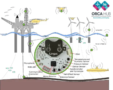
The UK Robotics and Artificial Intelligence Hub for Offshore Robotics for Certification of Assets (ORCA Hub) is a 3.5 year EPSRC funded, multi-site project with a vision to use teams of robots and autonomous intelligent systems (AIS) on remote energy platforms to enable cheaper, safer and more efficient working practices [1]. The ORCA Hub brings together top industrial companies (Total, Chevron, BP and many others) with academia (University of Edinburgh, Heriot-Watt University, University of Oxford, Imperial College London and University of Liverpool). The long-term vision for the ORCA Hub is an offshore platform that is completely autonomous and being operated and inspected from the shore, which will decrease the number of people working offshore. The ORCA Hub System constitutes the offshore platform, assets and the heterogeneous robotic systems (topside, aerial and marine robots) interacting with the platform as shown by Figure 1. The ORCA Hub System provides remote solutions using robotics and Artificial Intelligence (AI) that are readily integratable with existing and future assets and sensors, and that can operate and interact safely in autonomous or semi-autonomous modes in complex and cluttered environments [1]. The ORCA Hub System aims at achieving tasks that are not possible with a single robot due to the complex nature of offshore platforms. It includes many components such as robotic autonomy, mobility, manipulation, sensor processing, autonomous mapping, navigation, multimodal interfaces and human-machine collaboration. In this work, we focus on the sensing aspect of the ORCA Hub System. Sensing is a key element to the ORCA Hub System as it is important in asset monitoring, fault detection, mapping, environmental monitoring and helping other robots navigate around the platform.
1.4. Offshore Robotics (Current-State-of-the-Art and Challenges)
Robots on offshore platforms face many challenges. Some of these challenges include the absence of protection against saltwater spray and direct sunlight, harsh weather conditions involving rain, hail and high speed winds, extreme ambient temperature, high humidity levels, and dangerous atmospheric conditions resulting from gases, which can be explosive, toxic and corrosive [4]. For a robot to be suitable for operation on offshore platforms, there are some requirements regarding hardware, software and communication. Some of the hardware requirements for offshore robots include making the electronics suitable for harsh environments and equipping the robot with highly reliable sensors to perceive its surroundings [4]. Offshore robots also have requirements for software development including the ability to control the robot from remote locations, ease of programming new inspection and manipulation tasks without the use of experts, and the capability to alert remote operators when sensor values detected are abnormal [4]. Communication requirements mainly includes the ability to communicate and transmit data to a remote control station or to neighbouring systems. As a result of the harsh offshore conditions, remote sensing is becoming extremely valuable. Recent advances in the Internet of Things (IoT) and the cloud computing model provide support for remote sensing [5].
equipped with a robotic arm, a camera and several application sensors such as a microphone, gas sensor and fire sensor. The robotic prototype can autonomously execute pre-programmed inspection tasks in automatic mode.
1.5. Fault Detection and Condition Monitoring Systems
A potential application for robots on offshore platforms is fault detection and condition monitoring systems. Condition monitoring techniques help describe types of faults that can occur to a system, and the observable signs generated by these faults. Offshore implementation of fault detection and condition monitoring is challenging due to the complexity of remote sensing, data collection, data processing and data analysis. Condition monitoring systems play an important role in reducing maintenance and operational costs in offshore structures such as wind turbines. Technological advances in the development of wind turbine blades have led to an increase in the blade span, which increases the aerodynamic load on the blades and makes the blades more vulnerable to failure. The turbines also face harsh environmental conditions, which increases the chance of failure. Failure of wind turbines hinders the economic feasibility of offshore wind farms and, therefore, real-time condition-monitoring and fault detection for wind turbines is essential [19]. According to the Rules and Guidelines for Industrial Services, offshore wind turbines need to be equipped with blade condition monitoring systems to meet the safety requirements [20].
Different techniques for condition-monitoring of wind turbines have been proposed in the literature [21]–[26]. Some of these techniques for fault diagnosis of wind turbines are based on piezoelectric impact sensors [27], acoustic emission sensors [28], fibre Bragg grating sensor system [29], [30], piezoceramic and impedance sensing [19], [31]. However, real-time condition monitoring of wind turbines and fault detection has not been studied in great detail, due to the harsh environments surrounding wind turbines, which makes experimental research challenging. Our work introduces a novel method to achieve real-time condition monitoring and fault detection for offshore wind turbines by combining signal-processing methods with remote sensing. The reliability of the monitoring system is enhanced by conducting all the data processing and analysis on the microcontroller, and transmitting data using high-range low-bandwidth communication systems only in the event of the presence of a fault.
1.6. The Limpet
In this work, we introduce our new immobile multi-sensing robot, the Limpet, which is low-cost
and designed for manufacturability. Immobile robots (“Immobots”) were introduced by Williams
and Nayak in 1996 [32]. According to them, immobile robots are sensor-rich, distributed autonomous systems. Immobots were introduced as a third class of autonomous agents, along with mobile robots and soft robots, by AI researchers at the 1997 AAAI Workshop on Theories of Action, Planning and Control [33]. Examples of immobots include networked building energy systems, autonomous space probes, chemical plant control systems, satellite constellations for remote ecosystem monitoring, power grids, biosphere-like life-support systems, and reconfigurable traffic systems [32]. Such systems are considered immobile robots that exploit a vast system of sensors to model themselves and their environment on a grand scale [32]. Roush states that immobots could become pervasive,
where they can help control some of the world’s most important infrastructure technologies [34]. He
allows it to sense light and darkness levels [35]. We developed our bio-inspired robot, the Limpet, for inspection and monitoring of offshore energy platforms. We embedded permanent magnets in the protective housing of the Limpet to enable it to attach to metallic surfaces. The protective housing acts as a shell that protects the circuitry from the harsh offshore weather conditions. We can also integrate the Limpet with the Robot Operating System (ROS).
2. Design and Fabrication of the Limpet
2.1. Instrument Model
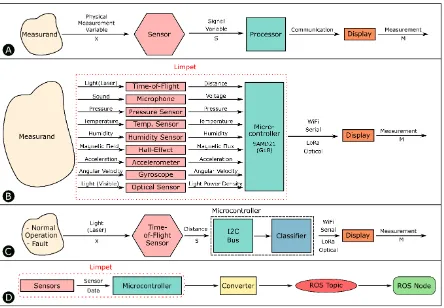
Figure 2. A) Instrument model. A measurand is the physical variable of interest that is represented by a physical measurement variable. The sensor converts the physical measurement variable into a signal variable that is fed to the microprocessor. Signal variables can be transmitted to an output device that is remote from the sensor. The value displayed is the measurement. B) The Limpet system overview. Our system, the Limpet, is a multi-sensing robotic platform, which is equipped with nine different sensors. The different physical measurement variables can be associated with several measurands. Each of the sensors on the Limpet converts a physical measurement variable into its corresponding signal variable. The signal variables are fed to the on-board microcontroller, which can then transmit the signal variable via one of several communication strategies (serial, WiFi, LoRa, optical) used by the Limpet. C) Instrument model for the Limpet for distance-based fault detection. We detect normal operation or the presence of a fault measurands by using light (laser) as a measurement variable. The time-of-flight sensor converts the time of arrival of the reflected light into a distance, which is fed to the microcontroller through the I2C bus. We apply the distance measurements to a classifier, which associates the measurements to one of the measurands. The result is transmitted to a remote PC using one of the four communication strategies. D) The Limpet and ROS Architecture. The sensor data from the Limpet is fed into the microcontroller. The microcontroller sends out the data to a converter, which converts this data into a ROS protocol. The data can be published to a ROS topic, and any ROS node can subscribe to that topic to read the sensor data.
transforms a physical variable of interest (measurand) into a form that is suitable for recording (measurement) as shown by Figure 2A. An example of a basic instrument is a ruler. In this case, the measurand is the length of some object, and the measurement is the number of units (meters, inches, etc.) that represents the length.
The measurand (physical process) is represented by an observable physical measurement variable (X). There is a wide range of physical measurement variables. Common physical measurement variables include: force, temperature, humidity, acceleration, velocity, pressure, frequency, time, length, capacitance, resistance, etc. It is important to know that the physical measurement variable (X) does not necessarily have to be the measurand, but can simply be related to the measurand. For example, the mass of an object is often measured by the process of weighing. In this case, the measurand is the mass but the physical measurement variable is the downward force the mass exerts in the Earth’s gravitational field. Another example is vibration detection. A robot can detect the measurand vibration by measuring force or by relating the measurand to another physical measurement variable such as acceleration. Both implementations will allow the detection of vibration, however, the accelerometer is much cheaper than the force sensor. There are also other situations where a single measurement variable contains information about multiple measurands. We refer to this capability as multi-functional sensing. One example is Infrared (IR) light. IR light has been used by robots for proximity measurements and communication with other robots [37]. Receiving signals from an IR transmitter requires sensors, such as photodiodes that transduce IR light into electric signals. Therefore, communication using IR light can be considered a sensing task. Another example is the use of the magnetic flux density from a single hall-effect sensor to detect whether the robot had a successful movement, collision or rotation measurands [38].
The key element of the instrument model is the sensor. The sensor’s function is to convert the physical measurement variable X into a signal variable S. Signal variables can be manipulated in a transmission system, such as an electrical or mechanical circuit, which means that they can be transmitted to an output device that is remote from the sensor. In our work, we use this property to be able to transmit the signal variable to a remote device using different communication or transmission systems. Typical signal variables include voltage displacement, current, force, frequency, light, pressure, etc. The output from the sensor is transmitted to a display or recording device, and the observed output is known as the measurement (M).
2.2. Design of the Limpet 2.2.1. System Design
We equipped the Limpet with nine exteroceptive sensing modalities. The sensors incorporated in the Limpet are temperature, pressure, humidity, optical, distance, sound, magnetic field, accelerometer and gyroscope. The Limpet can be modelled as an instrument, where each of its sensors converts a physical measurement variable into a corresponding signal variable as shown by Figure 2B. The signal variables are fed to the on-board microcontroller, which can then transmit the signal variable using one of several communication systems. In this work, we give one example of the multi-functional capabilities of the Limpet. Table 1 describes how the physical measurement from each sensor on the Limpet can be related to different measurands on offshore platforms. The table is based on the instrument model described in Figure 2A. It gives an example of a few potential measurands, and not all the measurands possible with each sensor.
Sensor
Physical Measurement
Variable
Signal Variable Measurands
Accelerometer Acceleration Acceleration
Inclination, Collision,
Vibration,
Free-Fall Detection,
Movement
Acceleration
Gyroscope Angular Velocity Angular Velocity Tilt Detection, Orientation
Temperature Temperature Temperature
Ambient
Temperature,
Over-heating, Fire Detection
Humidity Humidity Humidity Relative Humidity
Microphone Sound Voltage
Speech Recognition,
Noise Cancellation,
Audible Fault
Detection
Pressure Pressure Pressure Ambient Pressure
Hall-Effect Magnetic Field Magnetic Flux Density Locating Pipelines, Corrosion Detection
Optical Light (Visible) Distance
Ambient Light Intensity, Local Communication, Colour Detection
Distance
(Time-of-Flight) Light (Laser) Distance
Fault Detection, Proximity, Collision
Detection, Object Identification
In this work, we demonstrate the use of a distance sensor, which is a Time-of-Flight (ToF) sensor, for fault detection in equipment, specifically a wind turbine. Figure 2C indicates the instrument model for the Limpet as considered in this work. The measurands normal operation and fault can be related to the physical measurement variable light. We use the distance sensor on the Limpet, which converts the physical measurement variable light to a signal variable distance, which is fed into the
microcontroller’s I2C bus. We use the microcontroller to process the sensor data on-board and check
them against a classifier. We use the distance measurements to classify if the machine is operating normally, or if there is a fault in the machine hindering its performance. The Limpet can send the data to a PC using one of several different communication systems. We can then use spectral analysis on the data to further reduce the information density and classify the type of fault detected.
integrated TCP/IP protocol stack capable of giving any microcontroller access to the WiFi network, on the Limpet. We use Mosquitto [39], which implements a messaging protocol known as Message Queuing Telemetry Transport (MQTT), to send the data wirelessly from the Limpet to the PC. MQTT is a light-weight publish/subscribe messaging protocol used for remote communication. The received data can then be plotted in a real-time basis using Matlab, or saved on the PC and processed later.
We designed the Limpet to have robust communication. We can use multiple communication methods with the Limpet, including serial, WiFi, LoRa and optical communication. LoRa is a digital wireless data communication technology that enables long-range transmission with low power consumption [40]. LoRa technology is provided by the LoRa Alliance, which is a non-profit association of more than 500 member companies that are developing and promoting LoRaWAN open standard for IoT. We achieve optical communication with a combination of the RGB LED and the optical sensor on the Limpet. WiFi and serial communication do not allow robot-to-robot communication, unlike LoRa and optical communication. We incorporated a communication fail-over mechanism on the Limpet. If the primary communication method (WiFi) fails for any reason, the functions of the WiFi are assumed by a secondary communication module, which makes the system more fault-tolerant and robust in communication and data transmission.
The Limpet has an onboard programming port (JTAG). We programed the Limpet using a SEGGER J-Link programmer together with a JTAG Adapter (Olimex ARM-JTAG-20-10). We programmed it in C/C++ using Atmel Studio 7. We used the standard Universal Asynchronous Receiver-Transmitter (UART) protocol for communication. The UART protocol uses a high idle line, which is pulled low at the start of a message.
Cost and functionality were the most important factors that we considered when designing the Limpets. Our rationale behind the system design was to keep the costs as low as possible without sacrificing functionality. The Limpet has a diameter of 50 mm, a height of 7 mm and weighs 17g with, and 10g without, the battery. We designed the Limpets to have a size and weight ideal for ease of fabrication, manufacturing and assembly. The total cost of electronic components used in the design of the Limpet is about £22.
2.2.2. Electrical Design
The Limpet consists of a single two-layer Printed Circuit Board (PCB) and a detachable Li-Ion coin cell battery. We designed a fully integrated PCB incorporating a low –power microcontroller (ATSAMD21G18A), RGB LED (LTST-N683EGBW), battery holder (BK-877) for a rechargeable Li-ion battery (LIR2477), charging IC (MCP73812T), charger connector, programming port [JTAG] (Molex 532610571), and a communication connector as shown by Figure 1. The PCB includes several exteroceptive sensors, which are: Temperature and Humidity Sensor (Si7006), IMU [Accelerometer and Gyroscope] Sensor (LSM6DS3), Optical Sensor (VEML6040), Sound Sensor (SPU0414HR5H-SB), 3-Axis Magnetic Sensor (MLX90393), Pressure Sensor (BMP280), Distance Sensor (VL53L0). Figure S1 shows the PCB schematic. The communication connector is connected to UART of the microcontroller. Therefore, we can use this connector to connect the Limpet to different communication systems. We designed the Limpet to use a single PCB for control, communication and sensing.
The sensors on the Limpet, except for the microphone, are controlled by the microcontroller through the I2C bus. The microphone is an omnidirectional MEMS sensor, with an analogue output and a frequency range of 100 Hz to 10 KHz. In this work, we use the distance sensor for fault detection. The distance sensor on the Limpet is the smallest range sensor on the market today. It is a ToF laser-ranging module that can measure sub-mm distances for a range between 0 and 2.2m. We also demonstrate the use of the optical sensor for local communication between two Limpets.
approximately 182.9 mA (ESP8266 consumes 135 mA, RGB LED consumes 20 mA, sensors consume 20.9 mA, microcontroller consumes 7 mA), which allows for a battery life of about 0.87 hours or 52.2 minutes. We calculated the maximum battery life by assuming the Limpet is in sleep mode, where it consumes an average current of 0.1 mA. In this mode, the battery life of the Limpet can reach about 1600 hours or 67 days.
2.2.3. Mechanical Design
We designed the PCB of the Limpet using Eagle PCB Design Software and fabricated them on double-sided Cu-FR4-Cu 0.1-mm boards using an external company called Minnitron Ltd (Kent, United Kingdom). We purchased all electronic components from RS components and Digi-key Electronics. We soldered the components on the PCB using a reflow soldering process. In this process, we cut solder paste stencils from vinyl using a Laser Cutter (Epilog Laser Fusion 32).
We fabricated the protective housing from an optically clear, semi-rigid polyurethane resin. We developed the housing by casting the resin in a 3D printed mould. We did not cover the surfaces of the sensors by resin to keep them exposed to the external physical measurement variables. A picture of the encapsulated Limpet and the mould can be found in Figures S2 and S3.
We designed the Limpet explicitly for manufacturability; it consists of a single PCB and therefore mass manufacture is a simple case of placing a batch order with a PCB foundry. The PCB consists of surface mount components, except for the communication connector, and can be autonomously populated with pick-and-place machines at the point of manufacture. Robots that are made of a single PCB with mostly surface components allow for scaling up to huge collectives of robots easily without sacrificing functionality [41]. Assembly of one robot takes seconds as it is a matter of only connecting the coin cell battery. Once the battery is connected, there is no need to remove the battery from the robot again as it can be charged on-board. As a result of the Limpet being highly manufacturable and easy to assemble, it is easy to mass-produce Limpet agents and deploy them in huge collectives.
2.3. ROS Interface
We can interface the Limpet with ROS as shown by Figure 2D. The sensor data are fed into the microcontroller. The microcontroller sends out the data to a converter, which converts this data into a ROS protocol. We can publish this data to a ROS topic, and any ROS node can subscribe to that topic to read the sensor data. The different sensors on the Limpet have different physical measurement variables. When these measurement variables are fed into the microcontroller, it adds a label to the data to differentiate data from the different sensors (e.g. distance, temperature, pressure, etc). The data are published to the relative ROS topic based on this label as shown by Figure S4. ROS nodes can subscribe to relevant topics to gain access to the sensor data. Interfacing the Limpet with ROS enables it to interact with other robots in the ORCA System that are running ROS, where the interaction between them can result in a more complex and useful behavior. Figure S5 depicts the results from integrating the Limpet with ROS. It shows a screenshot of the data published to the distance ROS Topic, and a graph of the distance measurement from the ROS Topic during normal operation of the fan.
3. Experimental Design
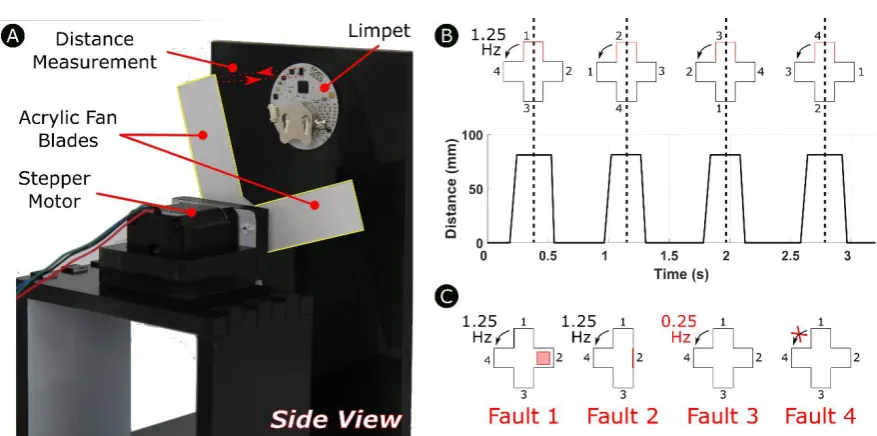
Figure 3. A) Experimental setup for distance-based fault detection. We fixed the Limpet in place and used the fan to mimic a small wind turbine. We attached the fan blades, which were cut out of acrylic sheets, to a stepper motor to achieve rotation. We fixed the stepper motor in place to minimize the errors in measurement by having the fan at the same distance from the Limpet for all the experiments. B) Schematic of the fan and distance profile for nomal operation mode. Each peak corresponds to one of the four fan blades detected. The time period corresponds to the frequency of detection of the fan blades. The absence of a fan blade in front of the Limpet corresponds to a measurement of zero. C) Schematic of the faults introduced to the system.
3.1. Design of the Distance-Based Fault Detection Experimental Setup
The experimental setup consists of a platform containing the Limpet and a custom-designed fan with four blades rotating in front of the Limpet as shown by Figure 3A. We designed the fan blades by cutting a pattern out of an acrylic sheet using a laser cutter. We attached the fan blades to a stepper motor to achieve rotation. We used the fan to mimic a small wind turbine. We placed the fan at a distance of 85 mm from the Limpet. We use the ToF sensor on the Limpet to measure distance to the fan blades as they are rotate. We fix the Limpet in place on a small wall in front of the fan to reduce the chance of errors in the distance measurement due to any displacement by the Limpet. We controlled the speed of rotation of the fan by controlling the speed of rotation of the stepper motor. When a blade passes in front of the Limpet, the blade is intercepted by the ToF sensor, and a distance measurement is recorded. We programed the Limpet to interpret the absence of a blade as a zero measurement. One of the errors we face in our experiment is that the distance sensor detects the edge of the fan blade as it is approaching the sensor, since the sensor has a Field of View (FoV) of 25˚. This error results in a larger number of distance measurements versus time as each blade passes in front of the limpet. Figure 3B shows a schematic of how the distance measurement was determined for the fan for normal operating conditions. It shows the distance profile, which depicts the distance measurement for each blade passage in front of the Limpet. The frequency of detection of the fan blades is 1.25 Hz under normal conditions. The fan has four blades, and each blade corresponds to a peak on the graph. In our case, the zero value represents the absence of a blade in front of the Limpet. We recorded the distance profile over a period of 3.2s, which corresponds to the frequency of rotation of the fan. The difference in width between the peaks is due to the error in detection of the edges of the blade..
3.2. Overview of the Communication
communication bandwidth is high, and we can send the sensor data from the Limpet continuously in real time to the PC. We can then analyse the data on the PC using analysis tools such as Matlab. In this regard, the Limpet is only making a measurement and transmitting it instantly to the PC without doing any processing on the data, which means serial and WiFi communication are not computationally demanding on the Limpet. We transmit the data from the Limpet over WiFi using
the ESP8266, and serially using SparkFun’s FTDI Basic Breakout - 3.3V, which is a serial to USB
convertor.
LoRaWAN is a new wide area network (WAN) technology that allows for long-range communication, but with a limited bandwidth. Low power WAN combines robust modulation and low data rate to achieve long range communication. LoRaWAN is one of the most successful tools in low power WAN technologies. It is a network stack rooted in the LoRa physical layer. LoRaWAN features a low data rate (a maximum of 27 kb/s with spreading factor 7 and 500 kHz channel) and long range communication (2–5 km in urban areas and 15 km in suburban areas). There is a tradeoff between the spreading factor and communication range in LoRa. The higher the SF, which means the slower transmission, the longer the communication. Depending on the spreading factor used (7 to 12), LoRaWAN data rate ranges from 0.3 kb/s to 27 kb/s [42]. LoRa has a much lower communication bandwidth than serial and WiFi communication. Thus, when we use LoRa technology with the Limpet for communication, the limited bandwidth limits the ability to send the sensor data continuously in real time to the PC. Therefore, if the dataset is large, processing and analysis of the data need to be done before transmission to allow for only small amounts of data to be transmitted. This on-board processing and analysis approach requires higher computational power than serial and WiFi communication. We used the LoPy, which is a MicroPython enabled WiFi, Bluetooth and LoRa development board, to gain access to the LoRa network. The LoPy transmits the data from the Limpet to The Things Network, which is a network that uses LoRaWAN to allow for devices to talk to the Internet without 3G or WiFi.
Optical communication has the lowest bandwidth among the four communication strategies. The processing and analysis also need to be done before the transmission of data. In our case, we transmitted data using the on-board RGB LED. We transmit the data by pulse-width modulating (PWM) the LED to different levels, where each level corresponds to a number from 0 to 9. We used the different LED colours to correspond to different measurements such as time, distance, pressure, temperature, etc. We used the optical sensor to read the light intensity and colour power density, in order to interpret the data transmitted using the RGB LED. There is an extra step involved in the optical communication, which is the calibration and use of the optical sensor to infer the transmitted data. This extra step implies a higher computational power demand for optical communication. Optical communication can not be used for long-range communication, but can be used for communication with underwater vehicles, as blue light can propagate seawater better than other types of light [43].
3.3. Design of the Classification Techniques 3.3.1. Signal Processing Tools
To eliminate outliers from the input signal, we applied a Median Absolute Deviation (MAD) Algorithm. MAD algorithm is used in statistics as a measure of the variability of a sample of quantitative data. MAD is more resilient to outliers in a dataset than the standard deviation. Since MAD is more robust to scale estimates than the standard deviation, it is better applied to data that is not normally distributed, which is the case in this work. Consider an input signal 𝑥 = [𝑥1, … , 𝑥𝑁]
with length N. MAD is defined as the median of the absolute deviations from the dataset’s median,
and is given by
𝑀𝐴𝐷 = 𝑚𝑒𝑑𝑖𝑎𝑛 (|𝑥𝑖− 𝑚𝑒𝑑𝑖𝑎𝑛(𝑥)|), 𝑖 = 1, … , 𝑁 (1)
After the successful elimination of outliers, we applied a low pass filter to the data to remove white noise from the input signal. We applied a simple moving average filter to smooth out the short-term fluctuations in the data. In this stage, we calculate the mean from an equal number of data points on either side of a central value. By doing so, the variations in the mean are associated with the variations in the data instead of being shifted in time.
For an input signal x and a positive integer k, the moving average y is computed by sliding a window of length k along x. Each element of y is the local mean of the corresponding values in the input signal x within the window, and signal y is the same size as x. For a signal x made up of k scalar observations, the mean µ and the moving average y are given by
µ =1
k ∑ 𝑥𝑖
𝑘
𝑖=1
(2)
𝑦 = [µ𝑖, … , µ𝑁] (3)
We have chosen a moving average sliding window of size (k=8) as the distance sensor records 8 data points for each blade passage in front of the sensor due to sampling frequency we set for the sensor (25 Hz). The time series after application of the low-pass filter varies within a narrower range as compared to the signal after elimination of outliers.
After elimination of outliers and noise, we reduce the input signal 𝑥 = [𝑥1, … , 𝑥𝑁] with length N in size to accord with the computational limitations of the microcontroller. We reduce the length of the signal from N to M by dividing the signal into M parts, each of which contains 𝐿 =𝑁
𝑀 measurements. The value of each element 𝑥𝑀′ of the down-sampled signal 𝑥′ is given by
𝑥𝑚′ =1
𝐿 ∑ 𝑥𝑖
𝐿𝑚
𝑖=𝐿(𝑚−1)
, 𝑚 = 1, … , 𝑀 (4)
In this work, we down-sample the full distance measurement for each fan rotation to 8
measurements (M = 8) corresponding to the four peaks in the distance profile. We conduct the same process on the timestamp and index information sent with the original data. Down-sampling has an
impact on the classifier’s detection rate. The higher the down-sampling frequency on the input
signal, the worse the detection rate becomes. Down-sampling potentially removes important features in the signal that can help the classifier discriminate between signals constituting normal operation or a fault. However, the higher the down-sampling frequency, the lower the memory required to store values of the cumulative distance matrix. Memory reductions are useful since it lowers the requirements for our low-cost microcontroller. Therefore, there is a tradeoff between memory reduction and classifier performance. In this work, we were able to achieve good classification performance with suitable memory usage as shown in the Results Section. We determined the down-sampling frequency after conducting multiple experiments for normal operation of the fan and studying the signal for characterising features in the distance profile.
3.3.2. Analysis Tools
After processing the input signal, we use spectral analysis to classify the fault detected. Spectral analysis has been used extensively in literature for fault detection [44], [45]. We first apply a fast Fourier Transform (FFT) algorithm to the processed signal, which divides the time signal into its frequency components. These components are single sinusoidal oscillations at different frequencies, where each component has its own phase and amplitude. The FFT algorithm is the Discrete Fourier Transform (DFT) of a sequence. FFT computes the same results as DFT, but can do it more quickly. In terms of time complexity, which is described as the amount of time needed to run an algorithm based on its computational complexity and expressed using big O notation, DFT takes O(N2) arithmetical operations, while FFT takes O(N log N) arithmetical operations for an input signal with N points. The N-point DFT equation for a finite-duration sequence x(n) is given by
𝑋(𝑓) = ∑ 𝑥(𝑛)𝑒−𝑗2𝜋𝑁 (𝑓−1)(𝑛−1), 1 ≤ 𝑓 ≤ 𝑁
𝑁
𝑛=1
Following the application of the FFT algorithm, we compute the power spectral density function (PSD) of the signal. The PSD shows the variation of power as a function of frequency, which could be used to detect abnormal system behaviour. Thus, observing the PSD of the recorded sensor data will enable classifiying the fault using a single parameter. The power spectral density for a signal x(n) with N points is given by
𝑃(𝑓) = 1
𝑁 |𝑋(𝑓)|
2 (6)
For a periodic rectangular pulse function, the FFT divides the pulse signal into several harmonics (sine waves) to approximate the pulse signal. Adding more sine waves of increasingly higher frequencies improves the approximation of the rapid changes (discontinuity) in the pulse signal. In the frequency domain, a periodic rectangular pulse function results in a sinc() function centered around the dominant frequency. As the duty cycle or pulse width of the signal is varied, the sinc() function changes. As the duty cycle is decreased, the width of the of the sinc() function broadens (i.e. it becomes less localised in frequency). Thus, if a function changes rapidly in time, the signal must contain high frequency component to allow for such a rapid change.
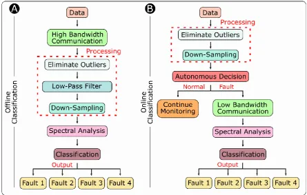
Figure 4. Overview of the signal processing components for A) Offline Classification and B) Online Classification.
3.3.3. Offline Classification
During normal operation of the fan, we compute the average and standard deviation of the distance measurements recorded over a period of ten minutes. We used these values as learning values for the microcontroller when performing the online classification process.
3.3.4. Online Classification
Figure 4B gives an overview of the online classification process. The Limpet starts sampling the distance to the fan using the ToF sensor. The Limpet stores a number of distance measurements into its memory (120 measurements). The Limpet processes the data, by first removing any outliers from the sensor data. The data are then down-sampled according to the down-sampling frequency. The Limpet classifies the dataset using a sliding window algorithm. The sliding window algorithm is used to process data streams, where the input is presented as a sequence of items, and the function of interest is computed over a fixed-size window in the stream [46], [47]. The Limpet detects the first rising edge and the fourth falling edge and calculates the time period between them. This time period is checked against the frequency of normal operation stored in the microcontroller’s memory. The distance measurements are also compared to the average value and standard deviation of normal operation, which were stored in the microcontroller after training the classifier offline.
According to the offline training of the classifier, the distance measurement for each blade must fall within a range of average ± standard deviation. The parameters of the class representations (average, standard deviation, time period) were trained offline and do not change during operation. These parameters are stored on the Read-Only Memory (ROM) of the microcontroller. The amount of ROM used depends mainly on the number of points (120) in the dataset and their size (distance is 8-bit, time is 16-bit, distance index is 8-bit). After the Limpet checks the dataset for the presence of any faults, it makes an autonomous decision based on the result of the classification. Autonomy is the ability of a system to make its own decision and to act on its own without external intervention [48]. Within autonomy, there are many variations concerning where and how decisions are made, and actions are invoked. An automatic system carries out a number of fixed and prescribed activities, where there may be options, but they are fixed in advance and follow a rigid cycle [48]. An adaptive system uses feedback from the environment to improve its performance [48]. A completely
autonomous system makes decisions based on the system’s view of the situation at the time of
decision and its current view of the environment [48]. Decisions made by completely autonomous systems mimic human-level decisions.
Since the Limpet carries out a number of prescribed activities or checks during online classification, it can be considered an automatic system. If the dataset is within the specified range and frequency, the Limpet continues monitoring the system, but if the dataset fails any of the checks, the Limpet classifies the measurements as faulty operation. The Limpet then transmits the processed data using low bandwidth communication systems such as LoRa and optical communication to the PC, where spectral analysis is performed to classify the fault detected.
3.4. Design of the Distance-Based Fault Detection Experiments
To evaluate the capability of distance-based fault detection using the Limpet, we conducted five experiments for each of the four communication systems. We conducted the five experiments separately and repeated using each communication system. We designed one of the five experiments to be normal operation of the fan. In the other four experiments, we introduce a fault to the system and check if the Limpet is capable of detecting this fault. The faults introduced to the system are listed below and a schematic of these faults are shown by Figure 3C.
• Fault 1: We attach an object of 15 mm thickness to one of the four blades. • Fault 2: We remove one of the four blades of the fan.
• Fault 3: We reduce the frequency of detection of a fan blade from 1.25 Hz to 0.25 Hz.
• Fault 4: We immobilise the rotation of the fan for a certain time period during the course of its normal operation.
recorded the sensor data over a period of 300s.We processed the data and observed the distance profile from each experiment. We then analysed the data using spectral analysis to classify the type of fault that occurred during operation. To test for other faults we conducted two additional experiments using WiFi communication and serial communication, these were: sampling at a rate lower than the Nyquist Frequency, and immobilising the fan twice during the 300s measurement period.
For LoRa and optical communication, the Limpet follows the online classification approach where it does all the processing and analysis on-board, and then takes an autonomous decision based on the classification result. For optical communication, we designed an experimental setup, where we placed another Limpet in front of the Limpet that is part of the distance-based fault detection experimental setup. We aligned the second Limpet such that it does not block the distance sensor of the first Limpet, but at the same time with its optical sensor aligned with the RGB LED of the first Limpet. We used the down-sampled results from the LoRa and optical communication experiments to construct the distance profile for each experiment, and we perform a spectral analysis on the data to classify the type of fault present in the system.
Before we conducted any experiments using optical communication, we ran a calibration experiment for the light sensor, where we PWM the RGB LED from 0 to 255 in steps of 25. Each PWM level corresponds to a number between 0 and 9. We pulse-width modulated the red LED first, followed by the green LED and the blue LED. We used the optical sensor to read the light intensity and colour power density of the LED for each PWM level, and the results are shown by Figure S7. Plots of the power density versus time for different numbers transmitted using the red, green and blue LED are shown by Figures S8, S9 and S10, respectively. We used the results of this calibration experiment as a reference to interpret the data transmitted by the Limpet during the experiments with optical communication. We used the red LED to send distance measurements, the green LED to send timestamps, and the blue LED to send the index of the data point. Figure S11 shows a plot of the power density from each LED, which could be used to interpret the number transmitted for each measurement variable during the experiment.
4. Results
4.1. Distance-Based Fault Detection
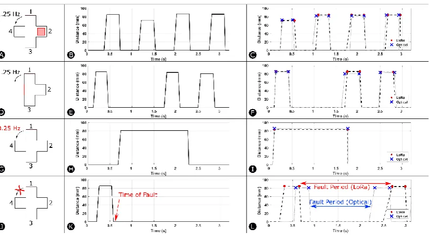
communication experiment for Fault 3. I) Distance Profile of LoRa and optcial communication experiment for Fault 3. J) Schematic of Fault 4. K) Distance Profile of WiFi communication experiment for Fault 4. L) Distance Profile of LoRa and optcial communication experiment for Fault 4.
Figure 5 depicts the results of the experiments for WiFi, LoRa and optical communication. It shows the distance profile resulting from each of the four faults introduced to the system. We constructed the distance profile for LoRa and optical communication (dotted lines) from the down-sampled results of the experiments (markers). Every two consecutive points (markers) on the graph represent a single peak or a fan blade. The distance profiles are shown within a period (T) of 3.2s (corresponding to the frequency of rotation of the fan during normal operation). When a fault is introduced to the fan and stepper motor system, its distance profile looks distinctly different as compared to the distance profile of normal operation. Each fault also possesses a distinctive power spectral density plot as compared to other faults.
Figure 5A shows a schematic of Fault 1. Figure 5B shows the distance profile acquired using WiFi communication, and Figure 5C shows the distance profile for LoRa and optical communication, after we introduce Fault 1 to the system. As seen in both Figures, one of the peaks in the distance profile has an amplitude lower than the other peaks as a result of the object attached (extra thickness) to it. Figure 5D shows a schematic of Fault 2. The results for WiFi communication, and LoRa and optical communication are shown by Figures 5E and 5F, respectively. The results of the three communication systems show that one of the peaks in the distance profile is missing as compared to normal operation. Figure 5G shows a schematic of Fault 3, where we reduced the frequency of detection of the fan blade to 0.25 Hz. The distance profile for WiFi, LoRa and optical communication shows only a single peak within 3.2s as shown by Figures 5H and 5I, as the frequency of blade detection is lower than normal operation. Figure 5J shows a schematic of Fault 4, where we immobilized the fan during its normal operation. The distance profile for WiFi communciation shows the absence of any peaks after the introduction of the fault to the system as shown by Figure 5K. Figure 5L shows the down-sampled results and the distance profile for LoRa and optical communication. The graph shows that two of the peaks are missing corresponding to where the fault is present. The fault period is slightly different for LoRa and optical communication experiments. The fault duration is also different for LoRa and optical communication as compared to WiFi communication. For WiFi communication, we recorded the distance measurements for a long period, and, thus the fault was introduced over a larger time window.
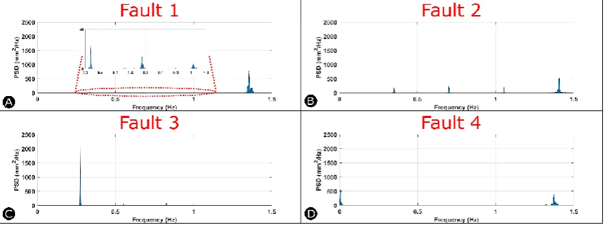
Figure 6. Spectral analysis of the data after introducing A) Fault 1, B) Fault 2, C) Fault 3 and D) Fault 4 to the system.
Figure 6 shows the power spectral density plots for each of the four faults. We obtained these results from the experiments using WiFi communication. During normal operation, the spectral analysis gives a single output signal (peak) at a frequency of 1.3 Hz as shown by Figure S21, which corresponds to the dominating harmonic frequency that best describes the signal in the time domain. In the time domain, the distance profile is a periodic rectangular pulse signal, therefore, in the frequency domain the harmonics exist around the same frequency. This collection of similar harmonics results in a peak in the frequency domain that is distributed around the dominating frequency. Figure 6A shows the power spectral density graph resulting from the introduction of Fault 1 to the system. There is a large peak at a frequency of 1.3 Hz, and three smaller peaks at frequencies of 0.35 Hz, 0.7 Hz and 1 Hz. The peak at 1.3 Hz represents the dominant harmonic in the time domain signal, while the other peaks are present because of the harmonics introduced to the system due to the presence of Fault 1. The PSD divides the signal into its single sinusoidal components at the different frequencies. In this case, the time domain signal is more complex, since the pulse signal is not periodic anymore. Therefore, the harmonics in this signal are more complex and introduce lower frequency components to describe the signal in the frequency domain. Figure 6B shows the power spectral density graph resulting from the introduction of Fault 2 to the system. There is a large peak at a frequency of 1.3 Hz, and three smaller peaks at frequencies of 0.35 Hz, 0.7 Hz and 1.1 Hz. The peak at 1.3 Hz represents the dominating harmonic in the time domain signal, while the other peaks are present because of the harmonics introduced to the system due to the presence of Fault 2. The absence of the peak in the time domain signal introduces new harmonics in the spectrum represented by the lower frequency components. This power spectrum is distinct from the power spectrum of Fault 1, as the power in the lower frequency harmonics is higher due to the larger difference in the amplitude between the peaks in the distance profile. The spectral analysis of Fault 3 shown by Figure 6C depicts a single large peak at a frequency of 0.25 Hz, which corresponds to the lower frequency of detection of the fan blades. The signal is a periodic rectangular pulse signal, and thus, results in a spectral plot with a peak around the dominant frequency. Since the duty cycle is increased as compared to normal operation, the peak is narrower and larger in the frequency domain. The spectral analysis of Fault 4 shown by Figure 6D depicts a large peak at a frequency of 1.3 Hz representing the normal fan operation and another peak at a lower frequency representing the break of rotation of the fan. The amplitude of the peaks depends on the length of the jam introduced to the system. Figure S22 shows the power spectral density plots from the WiFi experiments plotted against time.
Figures S23 and S24 shows the power spectral density plots from the serial communication experiments plotted against frequency and time, respectively. The results of the spectral analysis on the serial communication experiments are similar to the spectral analysis of the WiFi experiments. Figure S25 shows the optical sensor data, which is obtained from the transmission of measurements using the RGB LED during the optical communication experiments, and which shows the down-sampled results from the experiments and the spectral analysis performed on the data for both LoRa communication and optical communication after we introduce the four faults to the system. The frequency of the peaks in the power spectral density graph of LoRa and optical communication experiments are similar to those of serial and WiFi experiments. The only difference is the amount of power or energy in each peak. The power in the sinusoidal oscillations is much higher in serial and WiFi experiments as the results were recorded over a larger time period. The results from the two additional experiments (jamming the fan twice and a lower rate of sampling) we conducted using WiFi communication and serial communication are shown by Figures S26, S27, S28 and S29.
5. Discussion
explicitly adapted to operate on our low cost hardware. We introduced a down-sampling method to reduce the time taken to run the classifier and also to decrease the size required in memory on the microcontroller. We performed a sliding window algorithm on-board as a rapid test of the system’s functionality. The same approach can be applied to other sensors, which is discussed in section 5.1. The advantages and disadvantages of on-board computation as compared to offline computation are discussed in section 5.2.
5.1. Applicability to Other Sensors
In this work, we have shown how we can use a single sensor to monitor the state of equipment by measuring several measurands, as well as how we can process the data and analyse it on-board to improve communication requirements. Our method is dependent on distinct measurement profiles associated with each measurand. The method also depends on time-varying measurements. We think that this approach is applicable to other sensors and systems, if the measurement profile is (i) a time-varying measurement and (ii) distinctly different from other profiles. Thus, this method could be used by other sensors to identify different types of faults with equipment or to monitor different parameters on offshore platforms. It could also be easily adapted to other low cost systems.
5.2. On-board Data Processing vs Offline Processing
By processing and analysing data on-board using the microcontroller, we can improve the communication and power requirements of the system while still being able to perform same analysis. Data transmission does not need to occur continuously, but only in the case of a particular event. This design allows us to use communication systems with high transmission distance, but low bandwidth (such as LoRaWAN), and increase battery life of systems as the data transmission link is the most power-consuming part of a system. Offline processing involves continuously transmitting data and analyzing it to detect the presence of any faults. This approach is time-consuming, reduces battery life and requires high communication bandwidth, which lowers transmission distance. The major drawback of our approach is that low cost hardware is limited in its computational power. As such, we are restricted to the types of algorithms that could be used on the system.
6. Conclusions
Supplementary Materials: The following are available online at www.mdpi.com/xxx/s1, Figure S1: title, Table S1: title, Video S1: title.
Author Contributions: Created the system and is the lead author of the work, M.E.S.; Worked on the introduction literature, experimental design and advised on the development of the classifier, M.P.N.; Worked on the experimental design, introduction literature, classification and analysis and advised on the development of the classifier, S.A.; ROS Interface, A.C.M. and R.M.M.; Lead advisor and primary editor of the manuscript, A.A.S.
Funding: Markus Nemitz gratefully acknowledges support from the CDT in Intelligent Sensing and Measurement (EP/L016753/1), UK. Adam A. Stokes, Simona Aracri and Alistair C. McConnell acknowledge support from the EPSRC ORCA Hub (EP/R026173/1). Ross M. Mckenzie acknowledges support from EPSRC via the Robotarium Capital Equipment, and CDT Capital Equipment Grants (EP/L016834/1).
Conflicts of Interest: The authors declare no competing financial interest.
References
[1] H. Hastie et al., ‘The ORCA Hub: Explainable Offshore Robotics through Intelligent Interfaces’, in 13th Annual ACM/IEEE International Conference on Human Robot Interaction, 2018.
[2] J. W. Griggs, Energy law journal., vol. 32, no. 1. Federal Energy Bar Association, 2011.
[3] A. Shukla and H. Karki, ‘Application of robotics in offshore oil and gas industry— A review Part II’, Rob. Auton. Syst., vol. 75, pp. 508–524, Jan. 2016.
[4] H. Chen, S. Stavinoha, M. Walker, B. Zhang, and T. Fuhlbrigge, ‘Opportunities and Challenges of Robotics and Automation in Offshore Oil & Gas Industry’, Intell. Control Autom., vol. 05, no.
03, pp. 136–145, Jul. 2014.
[5] G. Mois, S. Folea, and T. Sanislav, ‘Analysis of Three IoT-Based Wireless Sensors for Environmental Monitoring’, IEEE Trans. Instrum. Meas., vol. 66, no. 8, pp. 2056–2064, Aug. 2017.
[6] J. Yuh and R. Lakshmi, ‘An intelligent control system for remotely operated vehicles’, IEEE J. Ocean. Eng., vol. 18, no. 1, pp. 55–62, 1993.
[7] J. Elvander and G. Hawkes, ‘ROVs and AUVs in support of marine renewable technologies’, in 2012 Oceans, 2012, pp. 1–6.
[8] G. A. Raine and M. C. Lugg, ROV Inspection of Welds - A Reality. Houston; TX: Underwater Intervention ’95, 1995.
[9] L. L. Whitcomb, ‘Underwater robotics: out of the research laboratory and into the field’, in Proceedings 2000 ICRA. Millennium Conference. IEEE International Conference on Robotics and Automation., 2000, vol. 1,
pp. 709–716.
[10] M. S. Wallace Bessa, ‘Controlling the dynamic positioning of a ROV’, in Oceans 2003, 2003, p. Vol.2. [11] P. E. Hagen, T. G. Fossum, and R. E. Hansen, ‘Applications of AUVs with SAS’, in OCEANS 2008, 2008,
pp. 1–4.
[12] M. J. Costa, P. Goncalves, A. Martins, and E. Silva, ‘Vision-based assisted teleoperation for inspection tasks with a small ROV’, in 2012 Oceans, 2012, pp. 1–8.
[13] M. Bengel and K. Pfeiffer, ‘Mimroex mobile maintenance and inspection robot for process plants’, 2007. [14] NREC/CMU, ‘Sensabot: A Safe and Cost-Effective Inspection Solution’, J. Pet. Technol., vol. 64, no. 10,
pp. 32–34, Oct. 2012.
[15] E. Kyrkjebo̸, P. Liljebäck, and A. A. Transeth, ‘A Robotic Concept for Remote Inspection and Maintenance on Oil Platforms’, in ASME 2009 28th International Conference on Ocean, Offshore and Arctic Engineering, 2009, pp. 667–674.
Congresso Brasileiro de Automática, 2014.
[17] A. F. Moghaddam, M. Lange, O. Mirmotahari, and M. Høvin, ‘Novel Mobile Climbing Robot Agent for Offshore Platforms’, Int. J. Mech. Aerospace, Ind. Mechatron. Manuf. Eng., vol. 6, no. 8, 2012.
[18] M. Bengel, K. Pfeiffer, B. Graf, A. Bubeck, and A. Verl, ‘Mobile robots for offshore inspection and manipulation’, in 2009 IEEE/RSJ International Conference on Intelligent Robots and Systems, 2009, pp. 3317–
3322.
[19] K.-Y. Oh, J.-Y. Park, J.-S. Lee, B. I. Epureanu, and J.-K. Lee, ‘A Novel Method and Its Field Tests for Monitoring and Diagnosing Blade Health for Wind Turbines’, IEEE Trans. Instrum. Meas., vol. 64, no. 6,
pp. 1726–1733, 2015.
[20] ‘GL Guideline for the Certification of Offshore Wind Turbines Edition 2012’, Hamburg, Germany, 2012. [21] W. Yang, P. J. Tavner, and M. R. Wilkinson, ‘Condition monitoring and fault diagnosis of a wind turbine
synchronous generator drive train’, IET Renew. Power Gener., vol. 3, no. 1, p. 1, 2009.
[22] R. C. Kryter and H. D. Haynes, ‘Condition monitoring of machinery using motor current signature analysis’, Power Plant Dyn. Control Test. Symp., vol. 20, no. 17, 1989.
[23] A. J. M. Cardoso and E. S. Saraiva, ‘Computer-aided detection of airgap eccentricity in operating three-phase induction motors by Park’s vector approach’, IEEE Trans. Ind. Appl., vol. 29, no. 5, pp. 897–901,
1993.
[24] Z. Hameed, Y. S. Hong, Y. M. Cho, S. H. Ahn, and C. K. Song, ‘Condition monitoring and fault detection of wind turbines and related algorithms: A review’, Renew. Sustain. Energy Rev., vol. 13, no. 1, pp. 1–39,
Jan. 2009.
[25] B. Lu, Y. Li, X. Wu, and Z. Yang, ‘A review of recent advances in wind turbine condition monitoring and fault diagnosis’, in 2009 IEEE Power Electronics and Machines in Wind Applications, 2009, pp. 1–7.
[26] S.-H. Shin, S. Kim, Y.-H. Seo, S.-H. Shin, S. Kim, and Y.-H. Seo, ‘Development of a Fault Monitoring Technique for Wind Turbines Using a Hidden Markov Model’, Sensors, vol. 18, no. 6, p. 1790, Jun. 2018.
[27] T. Yuji, T. Bouno, and T. Hamada, ‘Suggestion of Temporarily for Forecast Diagnosis on Blade of Small Wind Turbine’, IEEJ Trans. Power Energy, vol. 126, no. 7, pp. 710–711, 2006.
[28] T. Buono, T. Yuji, T. Hamada, and T. Hideaki, ‘Failure Forecast Diagnosis of Small Wind Turbine using Acoustic Emission Sensor’, KIEE Int. Trans. Electr. Mach. Energy Convers. Syst., vol. 5–B, no. 1, pp. 78–83, 2005.
[29] K. Schroeder, W. Ecke, J. Apitz, E. Lembke, and G. Lenschow, ‘A fibre Bragg grating sensor system monitors operational load in a wind turbine rotor blade’, Meas. Sci. Technol., vol. 17, no. 5, pp. 1167–1172,
May 2006.
[30] S. Tian et al., ‘Damage Detection Based on Static Strain Responses Using FBG in a Wind Turbine Blade’, Sensors, vol. 15, no. 8, pp. 19992–20005, Aug. 2015.
[31] J. Ruan, S. C. M. Ho, D. Patil, and G. Song, ‘Structural health monitoring of wind turbine blade using piezoceremic based active sensing and impedance sensing’, in Proceedings of the 11th IEEE International
Conference on Networking, Sensing and Control, 2014, pp. 661–666.
[32] B. C. Williams and P. P. Nayak, ‘Immobile Robots AI in the New Millennium’, AI Mag., vol. 17, no. 3, pp. 17–35, Mar. 1996.
[33] R. P. Goldman and C. Baral, ‘Robots, softbots, immobots: The 1997 AAAI Workshop on Theories of Action, Planning and Control’, Knowl. Eng. Rev., vol. 13, no. 2, pp. 179–184, 1998.
[34] W. Roush, ‘Immobots Take Control’, MIT Technology Review, Dec-2002.
Limpet (Patellidae and Fissurellidae)’, J. Molluscan Stud., vol. 56, no. 3, pp. 415–424, Aug. 1990.
[36] J. G. Webster, The Measurement, Instrumentation and Sensors Handbook, 1st ed., vol. 104, no. 25. CRC Press LLC, 1999.
[37] N. Farrow, J. Klingner, D. Reishus, and N. Correll, ‘Miniature six-channel range and bearing system: Algorithm, analysis and experimental validation’, in 2014 IEEE International Conference on Robotics and
Automation (ICRA), 2014, pp. 6180–6185.
[38] M. P. Nemitz et al., ‘Multi-Functional Sensing for Swarm Robots Using Time Sequence Classification: HoverBot, an Example’, Front. Robot. AI, vol. 5, p. 55, May 2018.
[39] R. A. Light, ‘Mosquitto: server and client implementation of the MQTT protocol’, J. Open Source Softw., vol. 2, no. 13, p. 265, 2017.
[40] N. Sornin, M. Luis, T. Eirich, T. Kramp, and O. Hersent, ‘LoRaWAN Specification 1.0’, 2015.
[41] M. P. Nemitz et al., ‘HoverBots: Precise Locomotion Using Robots That Are Designed for Manufacturability’, Front. Robot. AI, vol. 4, p. 55, Nov. 2017.
[42] F. Adelantado, X. Vilajosana, P. Tuset-Peiro, B. Martinez, J. Melia-Segui, and T. Watteyne, ‘Understanding the Limits of LoRaWAN’, IEEE Commun. Mag., vol. 55, no. 9, pp. 34–40, 2017.
[43] M. H.-C. Jin, J. M. Pierce, J. C. Lambiotte, J. D. Fite, J. S. Marshall, and M. A. Huntley, ‘Underwater Free-Space Optical Power Transfer: An Enabling Technology for Remote Underwater Intervention’, in
Offshore Technology Conference, 2018.
[44] M. El Hachemi Benbouzid, ‘A review of induction motors signature analysis as a medium for faults detection’, IEEE Trans. Ind. Electron., vol. 47, no. 5, pp. 984–993, 2000.
[45] M. Pineda-Sanchez et al., ‘Partial Inductance Model of Induction Machines for Fault Diagnosis’, Sensors, vol. 18, no. 7, p. 2340, Jul. 2018.
[46] J. Wang, R. Wang, and T. Li, ‘Analysis of the data streams trend in sensor network based on sliding window’, in 2012 IEEE International Conference on Computer Science and Automation Engineering (CSAE),
2012, pp. 224–228.
[47] M. Vafaeipour, O. Rahbari, M. A. Rosen, F. Fazelpour, and P. Ansarirad, ‘Application of sliding window technique for prediction of wind velocity time series’, Int. J. Energy Environ. Eng., vol. 5, no. 2–3, p. 105,
Jul. 2014.