Article
Mapping and attributing normalized difference
vegetation index trends for Nepal
Nir Y. Krakauer1*, Tarendra Lakhankar1, José D. Anadón2
1 Department of Civil Engineering and NOAA-CREST, The City College of New York, New York, USA;
2 Department of Biology, Queens College, New York, USA; [email protected]
* Correspondence: [email protected]; Tel.: +1-212-650-8003
Abstract: Global change affects vegetation cover and processes through multiple pathways. Long 1
time series of surface land surface properties derived from satellite remote sensing give unique 2
abilities to observe these changes, particularly in areas with complex topography and limited research 3
infrastructure. Here, we focus on Nepal, a biodiversity hotspot where vegetation productivity is 4
limited by moisture availability (dominated by a summer monsoon) at lower elevations and by 5
temperature at high elevations. We analyze normalized difference vegetation index (NDVI) from 6
1981 to 2015 semimonthly, at 8 km spatial resolution. We use a random forest (RF) of regression trees 7
to generate a statistical model of NDVI as a function of elevation, land use, CO2level, temperature,
8
and precipitation. We find that NDVI has increased over the studied period, particularly at low 9
and middle elevations and during fall (post-monsoon). We infer from the fitted RF model that 10
the NDVI linear trend is primarily due to CO2level (or another environmental parameter that is
11
changing quasi-linearly), and not primarily to temperature or precipitation trends. On the other hand, 12
interannual fluctuation in NDVI is more correlated with temperature and precipitation. RF accurately 13
fits the available data and shows promise for estimating trends and testing hypotheses about their 14
causes. 15
Keywords:random forest; regression tree; carbon fertilization; land cover change; climate change 16
1. Introduction 17
Vegetation is being impacted globally by widespread stressors and changes, including land 18
conversion to anthropogenic uses, climate change leading to heat and moisture stress, CO2fertilization,
19
nitrogen deposition, and the spread of pest and invasive species. While methods such as in situ 20
inventories, atmospheric trace gas measurement, and numerical modeling can provide valuable 21
insights into quantifying and attributing impacts [1–5], remote sensing of the land surface offers a 22
unique avenue for observing change in vegetation cover over large areas and timespans of days to 23
decades. Normalized difference vegetation index (NDVI), based on the relative surface reflectance in 24
red and near infrared wavelengths, is well correlated with cover of healthy vegetation [6], and regional 25
and global products based on different satellite sensors are available [7,8]. NDVI is negatively affected 26
by drought in warm regions [9–11] but has increased in response to warming in many temperate 27
and Arctic areas, which has resulted in longer growing seasons there [12–14]. For East and Central 28
Asia, NDVI was found to have increased from roughly 1982 to 1996, due to longer growing seasons, 29
and then decreased from 1997 to 2006, due to worsening aridity [15,16]. Urbanization, irrigation and 30
fertilization can also change NDVI [17,18]. Since the trends in most places are small in magnitude, the 31
remote sensing data need to be carefully processed to remove artifacts due to, for example, degradation 32
of the satellite sensors over the course of a mission [19]. 33
Here, we study trends in vegetation cover in Nepal (located at 26-31 °N, 80-89 °E) a least developed 34
country where the majority of the population is engaged in agriculture and is highly vulnerable to 35
climate change. Nepal is a biodiversity hotspot, due in part to the wide topographic and climatic 36
range found over relatively short distances, ranging from the Indo-Gangetic plain in the south to the 37
Himalayan peaks and the Tibetan Plateau to the north [20]. There have previously been several studies 38
of NDVI trends in the broader region. [21] found a generally increasing trend in spring NDVI over the 39
Hindu Kush-Himalayan region between 1982 and 2006. [22] analyzed NDVI seasonality between 1982 40
and 2006 for the Himalayas region, including Nepal, finding that the start date of the growing season 41
trended earlier while the end date did not change. [23] conducted cluster analysis to identify patterns 42
in mean and maximum warm-season NDVI between 2001 and 2016, finding mostly increasing trends 43
(greening), with decreasing trends (browning) most common between 4 and 5 km elevation. Similarly, 44
a study of NDVI trends in Yarlung Zangbo Grand Canyon Nature Reserve, Tibet between 1999 and 45
2013 [24] found that greening was concentrated at the lower elevations, below 3 km. Delayed green-up 46
in Alpine grasslands of the western Tibetan plateau may be due to declines in spring precipitation 47
[25,26]. 48
Limited research has been carried out on NDVI trends specifically in Nepal. [27] mapped forest 49
types in Manaslu Conservation Area and computed NDVI trends and correlations with temperature 50
and precipitation from a nearby meteorological station for 2000-2008. [28] found a significant increasing 51
trend in warm-season NDVI over the Koshi River Basin over 1982-2006, though with a decline between 52
1994 and 2000. 53
This research, therefore, has two main objectives. First, we describe trends in NDVI in Nepal 54
by elevation and season based on a long-term remote-sensing data product. Second, we attempt to 55
attribute trends and interannual variability to changes in climate, land use, and CO2concentration.
56
2. Methods 57
2.1. Data
58
2.1.1. NDVI 59
NDVI data was obtained from the NDVI3g.v1 time series, an update of the earlier NDVI3g.v0 60
[29] which provides NDVI values twice a month on a 1/12 degree (approximately 8 km) grid from July 61
1981 to December 2015. This dataset is derived from measurements by over a dozen Advanced Very 62
High Resolution Radiometers (AVHRR) that orbited on different satellites for parts of this time period. 63
It has been extensively processed to correct for artifacts resulting from causes such as instrument and 64
orbit drift and volcanic eruptions so to be suitable for analysis of climate change. The formula for 65
NDVI is (NIR−RED)/(NIR+RED), where NIR refers to reflectance in the AVHRR near-infrared 66
band (channel 2, 0.725-1.10µm) and RED to reflectance in the AVHRR red band (channel 1, 0.58-0.68
67
µm) [30]. Missing or suspect data in NDVI3g.v1 is flagged and filled in either by spline interpolation
68
or from an average of other years. 69
Despite quality control steps used to derive this product, we found occasional NDVI values that 70
were quite different from those at adjacent time periods, and which are therefore likely to be due to 71
satellite instrument or viewing condition artifacts [31]. We therefore smoothed the NDVI3g.v1 series 72
by subtracting the median seasonal cycle, applying a 3-point median filter, and adding the seasonal 73
cycle back. 74
2.1.2. Elevation 75
Elevation was obtained at 3 arcsecond (approximately 80 m) resolution from the United States 76
Geological Survey (USGS) and World Wildlife Foundation (WWF) Hydrological data and maps based 77
on SHuttle Elevation Derivatives at multiple Scales (HydroSHEDS) project. HydroSHEDS is derived 78
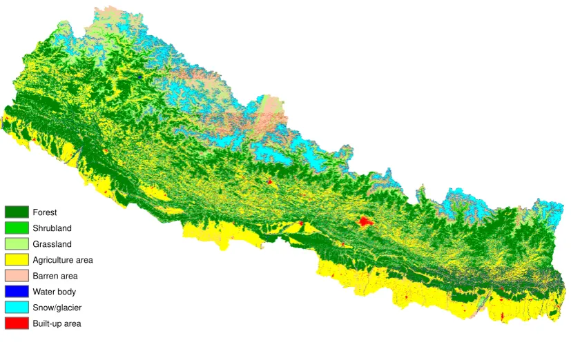
Table 1.Area coverage (%) of Nepal by land cover category and year.
Year Forest Shrub Grass Farm Barren Lake Snow/Ice Urban
1990 45.2 2.2 11.7 25.3 6.8 0.6 7.9 0.2
2000 41.7 2.4 11.4 27.7 9.5 0.5 6.5 0.3
2010 42.1 2.3 10.5 27.3 8.6 0.5 8.4 0.4
computed the average and standard deviation of elevation over each 1/12° grid cell in Nepal as 80
possible predictors of NDVI. Pixel-mean elevations ranged from 60 to over 6000 m (Figure1a), with an 81
average of 2078 m. 82
2.1.3. Climate 83
Monthly mean temperature and precipitation were obtained on a 1° grid. Precipitation was from 84
the Global Precipitation Climatology Center (GPCC) combined Full Version 7 and Monitoring Version 85
4 product, which is based on quality-controlled data from thousands of stations globally (including 86
data contributed by Nepal through the World Meteorological Organization) that is interpolated to fill 87
in gaps in coverage [33–35]. Temperature was from the Berkeley Earth (BEST) dataset, which uses 88
several times more station records compared to other gridded temperature data sets. Station records 89
undergo automated quality control, and are weighted using geostatistics methods to produce spatial 90
fields [36]. 91
The 1° resolution of these available products does not fully resolve the topography-driven 92
climate variability in Nepal. We mitigated this shortcoming, to some extent, by applying downscaling 93
adjustments. We downscaled the temperature data within each 1° cell to 1/12° by applying a lapse 94
rate of 6 K per km as an additive adjustment. This lapse rate was approximately that inferred from 95
the temperature difference between adjacent BEST pixels, which was found to be approximately the 96
same for all seasons. We downscaled the precipitation data within each 1° cell to 1/12° by applying 97
a multiplicative conversion factor based on the higher-resolution gridded APHRODITE product, 98
available for 1951-2007 in a public version at 0.25° resolution and, courtesy of the Nepal Department 99
of Hydrology and Meteorology, at the original 0.05° interpolation resolution [37]. These adjustment 100
factors were the same for each month, so that time trends were not affected, and preserved the 1° mean 101
values from GPCC and BEST. 102
The mean temperature and precipitation obtained, along with the elevation, for each 1/12° NDVI 103
pixel are shown in Figure1. 104
2.1.4. Land cover 105
Land cover classifications for 1990, 2000, and 2010 were obtained from the International Centre 106
for Integrated Mountain Development (ICIMOD) [38]. These were generated using public domain 107
Landsat Thematic Mapper 30 m images and an object-based classification algorithm, and validated 108
and refined using aerial photographs and field observations. The land cover classes were forest, shrub, 109
grass, agricultural, barren, lake, river, snow/glacier, and urban. We computed the percentage in each 110
cover category for each 1/12° pixel and year. Land cover was imputed by pixel and year via linear 111
interpolation between the three available years. Before 1990 and after 2010, we assumed the land cover 112
to have stayed constant at the earliest/latest available value. 113
The obtained land cover classification showed that forest (at almost half the area) and agriculture 114
(at about a quarter) were the dominant categories (Table1). Agriculture dominated in the lowest 115
elevations in the south, while forest dominated in the middle elevations, and grassland and snow and 116
glaciers were found at high elevations in the north (Figure2). Forest cover decreased by several 117
percentage points between 1990 and 2000 while agricultural and barren areas increased, before 118
2.1.5. CO2concentration
120
Yearly carbon dioxide dry air mixing ratios from Mauna Loa, Hawai’i (at 20° north, close to 121
Nepal’s latitude) was obtained from the United States Government’s Earth System Research Laboratory, 122
Global Monitoring Division. These are transformed to logarithms and can represent the impact of 123
increasing local carbon dioxide levels on plant gas exchange and carbon fixation. This time series is 124
also highly correlated to the summed anthropogenic greenhouse gas forcing [39], the global warming 125
trend [40], and other monotonic trends over recent decades, such as that of global population [41,42]. 126
2.2. Regression model
127
We expect the relationship of NDVI with such variables as temperature, precipitation and elevation 128
to be nonlinear. There also may well be interactions between potential explanatory variables, e.g. the 129
effect of precipitation increase could vary depending on elevation and season. Random forest (RF) of 130
regression trees [43] is a method of empirically constructing a predictive model that is well suited for 131
handling such complexity. As such, RF has been used in many environmental mapping applications, 132
including for wetland cover from radar imagery [44], water table dynamics and depth to groundwater 133
[45,46], and ecosystem light use efficiency [47]. Here, the training data were half of the available 134
1,429,443 NDVI values from Nepal (1955 pixels for 828 time periods, excluding 12% interpolated data). 135
The half the available data not used to train the model (test data) provided a test of its ability to capture 136
the NDVI patterns consistently found by remote sensing. The RF model run included 100 regression 137
trees, and other parameter settings were kept at default values from the RrandomForestpackage [48]. 138
The predictors in the RF model fell into the following categories: (1) Interannually constant 139
seasonal and geographic factors: month of year, pixel longitude, pixel latitude, pixel mean elevation, 140
pixel standard deviation of elevation. (2) Mean temperature (°C) for 0-0.5, 0.5-1.5, 1.5-3, 3-6, 6-12, 12-24, 141
and 24-48 months prior to the end of each semimonthly period. (3) Precipitation rate (mm month−1)
142
over the same periods as for temperature. (4) Land cover: percent of pixel in each of 8 land cover 143
categories. (5) Logarithm of atmospheric CO2concentration. The total number of predictors in the
144
model was therefore 5+7+7+8+1=28. 145
We then used the fitted model to predict NDVI trends if only one factor (temperature, precipitation, 146
land use, or CO2) changes with time, while the others are held at average values for the period (in the
147
case of temperature and precipitation, seasonally specific averages). To the extent that these factors 148
have different time histories so that their effects of NDVI can be separated by the RF model, this would 149
allow us to estimate how much of the NDVI trends and interannual variability over Nepal can be 150
attributed to each factor. 151
2.3. Analysis
152
For each grid cell and (semi-monthly) time of year, we computed the NDVI trend as the slope 153
obtained from linear regression, using only non-interpolated values. Trends were similarly computed 154
for the RF-predicted NDVI. The Nash-Sutcliffe coefficient [49], applied to different transformations 155
of the data, is used to quantify how well the RF models fit test data based on either the full set of 156
forcings or sets that include only one time-changing factor. NSCallis based on the raw observed and
157
modeled NDVI values (using only the test data), NSCdetrendis based on the same NDVI values, but
158
after subtracting the linear trend, which also removes the mean seasonal and spatial NDVI patterns 159
from consideration. NSCtrendis based on the linear trends (calculated using both training and test
160
data), and measures how well the RF model is able to capture the observed trend across space and 161
season. 162
Figure3shows graphically the overall workflow followed, including the relationship between 163
data processing and modeling. 164
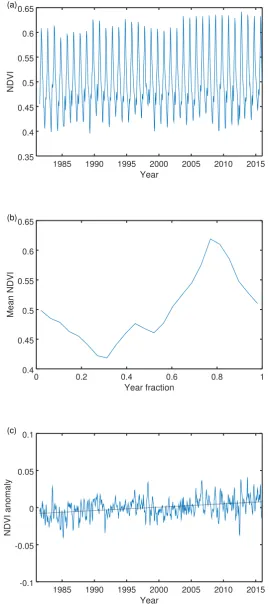
As one way of visualizing the results, we compute the time series of mean NDVI over Nepal by 165
predictions. The mean seasonal cycle is subtracted to obtain a deseasonalized time series for computing 167
trends and detrended variability. We also compute mean NDVI amounts and trends by season and 168
elevation, using a smoothing spline [50] to estimate the mean elevation dependence. 169
3. Results 170
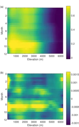
Mean NDVI was near 0 in the dry, cold high-elevation north of Nepal, which has little vegetation. 171
It was somewhat lower in the low plains near the India border compared to middle elevations, peaking 172
at about 0.65 over the elevation range 500-2000 m (Figure4). 173
The time series of mean NDVI is dominated by the seasonal cycle, though interannual variability 174
is also evident (Figure5). The mean NDVI seasonal cycle nationally and at elevations under∼4000 175
m was more influenced by moisture than by temperature, with peak values immediately after the 176
monsoon in early October. NDVI declines through winter, as water availability decreases, and reaches 177
a nadir in late April (Figure5b; Figure6a). At higher elevations (4000-5000 m), the peak occurs earlier 178
(late September) and the lowest values are in late February, consistent with a greater role of cold 179
temperature in controlling vegetation cover. 180
NDVI overall showed an increasing linear trend, averaging 0.448×10⁻³units per year, over the 181
period of record. This trend varied across seasons and elevations, however. It was strongest in late 182
August through October, near the annual peak, and in the lower elevations, below 2000 m (Figure6b). 183
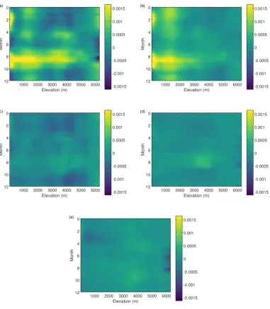
NDVI at 4000-5000 m actually showed a slight declining trend. 184
The RF model was able to represent the NDVI patterns seen extremely well (Figure7a), with 185
NSCallof 0.959 for the test data. However, most of this reflects skill at capturing the mean annual cycle
186
(Figure7b), rather than trends and year-to-year variability, so that even with no interannually-varying 187
forcings, the NSCallwas still 0.941. Out of the single forcings, CO2and precipitation contributed most
188
to improving NSCall, and temperature contributed least (Table2).
189
Interannual variability in NDVI after detrending was captured less well by the RF model (Figure 190
7c), with NSCdetrendof 0.288 for the test data. As expected, with no interannually-varying forcing,
191
none of this variability was captured. Out of the single forcings, precipitation contributed most to 192
NSCdetrend, with temperature playing a smaller role that was similar in importance to those of the
193
slowly varying CO2and land use (Table2).
194
The pattern of trends in NDVI across location and season was better captured by the RF model, 195
with NSCtrend of 0.793. With no interannually varying forcing, the trend was uniformly zero, as
196
opposed to the positive mean value actually seen, resulting in slightly negative NSCtrend. Out of the
197
individual forcings, CO2as well as land cover, which both changed quasi-linearly with time, explained
198
the trends best, with trends in temperature and precipitation showing smaller positive NSCtrend(Table
199
2). 200
Averaged over all Nepal, the mean NDVI trend from the fitted RF model was 0.422×10⁻³per 201
year, just 5% less than the 0.448×10⁻³calculated from the observation dataset. (Including all pixels 202
and months, also those missing from the observations, increases the mean trend calculated from the 203
fitted RF model slightly to 0.449×10⁻³per year.) This mean trend is indicated as being due essentially
204
to rising CO2level, which by itself raises NDVI 0.509×10⁻³per year. Land cover has a net negative
205
influence on NDVI trend, while precipitation and temperature trends have small positive influences 206
(Table2). 207
Figure8shows the modeled NDVI trend by season and elevation, which can be compared with 208
the observation-based trend in Figure6b. CO2change is the dominant factor at most of the affected
209
seasons and elevations. Land use change seems to have the largest impacts, which vary by season, 210
above 2000 m. Precipitation trends impact NDVI primarily during the monsoon season of summer 211
Table 2.Nash-Sutcliffe coefficients and mean trend for random-forest (RF) predictions of NDVI. The full RF model includes all time-varying factors. The other predictions are with either interannually constant factors or only one time-varying factor. The mean trend is in 10−3units per year. For comparison, the mean trend calculated from observations is 0.448×10⁻³per year.
NSCall NSCdetrend NSCtrend Trend
Full RF 0.959 0.288 0.793 0.422
Constant 0.941 -0.000 -0.068 0.000
CO2 0.946 0.053 0.344 0.509
Land cover 0.945 0.034 0.238 -0.135
Precipitation 0.946 0.102 0.043 0.020
(a)
80 82 84 86 88
26 27 28 29 30 31
E o N
o
1000 2000 3000 4000 5000 m
(b)
80 82 84 86 88
26 27 28 29 30 31
E
o N
o
0 5 10 15 20 25
o
C
(c)
80 82 84 86 88
26 27 28 29 30 31
E
o N
o
500 1000 1500 2000 2500 mm year -1
Forest
Shrubland
Grassland
Agriculture area
Barren area
Water body
Snow/glacier
Built-up area
Figure 2.2010 land cover map of Nepal.
80 82 84 86 88 26
27 28 29 30 31
o
E o N
0.1 0.2 0.3 0.4 0.5 0.6
1985 1990 1995 2000 2005 2010 2015 0.35
0.4 0.45 0.5 0.55 0.6 0.65
Year
NDVI
(a)
0 0.2 0.4 0.6 0.8 1
0.4 0.45 0.5 0.55 0.6 0.65
Year fraction
Mean NDVI
(b)
1985 1990 1995 2000 2005 2010 2015 -0.1
-0.05 0 0.05 0.1
Year
NDVI anomaly
(c)
(a)
1000 2000 3000 4000 5000 6000
0
2
4
6
8
10
12
Elevation (m)
Month
0 0.2 0.4 0.6
(b)
1000 2000 3000 4000 5000 6000 0
2
4
6
8
10
12
Elevation (m)
Month
-0.0015 -0.001 -0.0005 0 0.0005 0.001 0.0015
1985 1990 1995 2000 2005 2010 2015 0.35
0.4 0.45 0.5 0.55 0.6 0.65
Year
NDVI
(a)
0 0.2 0.4 0.6 0.8 1
0.4 0.45 0.5 0.55 0.6 0.65
Year fraction
Mean NDVI
(b)
1985 1990 1995 2000 2005 2010 2015 -0.1
-0.05 0 0.05 0.1
Year
NDVI anomaly
(c)
(a)
1000 2000 3000 4000 5000 6000 0
2
4
6
8
10
12
Elevation (m)
Month
-0.0015 -0.001 -0.0005 0 0.0005 0.001 0.0015 (b)
1000 2000 3000 4000 5000 6000
0
2
4
6
8
10
12
Elevation (m)
Month
-0.0015 -0.001 -0.0005 0 0.0005 0.001 0.0015
(c)
1000 2000 3000 4000 5000 6000
0
2
4
6
8
10
12
Elevation (m)
Month
-0.0015 -0.001 -0.0005 0 0.0005 0.001
0.0015 (d)
1000 2000 3000 4000 5000 6000
0
2
4
6
8
10
12
Elevation (m)
Month
-0.0015 -0.001 -0.0005 0 0.0005 0.001 0.0015
(e)
1000 2000 3000 4000 5000 6000 0
2
4
6
8
10
12
Elevation (m)
Month
-0.0015 -0.001 -0.0005 0 0.0005 0.001 0.0015
Figure 8.Modeled 1981-2015 linear trend in NDVI (10−3per year) for Nepal, by season and elevation,
with (a) all forcings, (b) only CO2level change, (c) only land use change, (d) only precipitation change,
4. Discussion 213
We find an overall increasing trend in NDVI for Nepal over 1981-2015. The RF analysis suggests 214
that this trend is not primarily due to changes in climate (temperature and precipitation), but 215
correlates best with increasing atmospheric CO2level, although precipitation and temperature are
216
more important in explaining interannual NDVI variability. Similarly, ecosystem models suggest that 217
most of the observed increase in the seasonal amplitude of atmospheric CO2, indicative of increasing
218
plant growth in the Northern Hemisphere over recent decades, is due to CO2 fertilization, with
219
climate and land use changes playing secondary roles [5]. An increasing trend in global net primary 220
productivity, particularly in tropical forests, has also been identified based on satellite imagery for 221
1982-1999 and attributed primarily to CO2fertilization [2]. On the other hand, in boreal areas, warming
222
has been a major driver of longer growing seasons and higher productivity [51,52], while in arid and 223
semiarid areas, moisture availability is a primary modulator of vegetation growth [15,53–55]. The 224
small positive impact of precipitation on NDVI trends, concentrated during and after the summer 225
monsoon, is consistent with the increasing trend in monsoon precipitation found for recent decades 226
over much of Nepal [56], although dry spells have also increased [57,58]. 227
Land cover change is inferred to have made a negative contribution to the NDVI trend. This is 228
plausible insofar as the land cover data show net decrease in forest area and increase in agricultural 229
area, where forest often has higher and more constant NDVI than agricultural land [59]. Although the 230
importance of anthropogenic land cover change as a driver of ecological impacts is widely recognized 231
[60–62], studies of global and regional NDVI trends over recent decades have generally concentrated 232
on climate drivers without explicitly accounting for the contribution of land cover change. An RF 233
model offers one method to distinguish the influence of all these factors, which operate simultaneously 234
around the world. 235
The work presented here has several significant limitations. The NDVI trends attributed to CO2
236
level in the RF model could well also reflect contributions from other factors that have been changing 237
quasi-linearly and whose quantitative evolution was not incorporated in the RF model. These may 238
include, for example, N fertilization due to direct application and deposition, irrigation, change in 239
crops planted, and management of grasslands and forests, and changes in cloud and aerosols, For 240
most of these terms, more work is needed to understand how they are changing over different parts 241
of Nepal. As well, the quality of some of the inputs used could be improved. Land cover change 242
could be evaluated from Landsat imagery before 1990 and after 2010. A precipitation product at higher 243
resolution, which could be based on remote sensing calibrated to available weather stations, would 244
better resolve the sharp elevation and orographic gradients within Nepal and thus help clarify the 245
impact of moisture stress [63–65]. 246
5. Conclusions 247
We find that NDVI has increased over the studied period in Nepal, consistent with global trends. 248
Increases were uneven, and concentrated at low and middle elevations and during fall (post-monsoon). 249
We infer from the fitted RF model that the NDVI linear trend is primarily due to CO2 level (or
250
another environmental parameter that is changing quasi-linearly), and not primarily to temperature 251
or precipitation trends. On the other hand, interannual fluctuation in NDVI is more correlated with 252
temperature and especially precipitation. RF accurately fits the available data and shows promise for 253
estimating trends in spatiotemporal remote sensing data such as gridded NDVI and testing hypotheses 254
about their causes. 255
Acknowledgments: The authors gratefully acknowledge support from USAID IPM IL under the
256
project “Participatory biodiversity and climate change assessment for integrated pest management in the
257
Chitwan-Annapurna Landscape, Nepal” and from NOAA under grants NA11SEC4810004 and NA15OAR4310080.
258
All statements made are the views of the authors and not the opinions of the funders or the U.S. government.
259
Author Contributions:All authors conceived and designed the data analysis and contributed analysis tools. NYK
260
performed the data analysis and wrote the paper.
Conflicts of Interest:The authors declare no conflict of interest.
262
References 263
[1] Caspersen, J.P.; Pacala, S.W.; Jenkins, J.C.; Hurtt, G.C.; Moorcroft, P.R.; Birdsey, R.A. Contributions of
264
land-use history to carbon accumulation in U.S. forests.Science2000,290, 1148–1151.
265
[2] Friend, A.D.; Arneth, A.; Kiang, N.Y.; Lomas, M.; Ogée, J.; Rödenbeck, C.; Running, S.W.; Santaren, J.D.;
266
Sitch, S.; Viovy, N.; Woodward, F.I.; Zaehle, S. FLUXNET and modelling the global carbon cycle. Global 267
Change Biology2007,13, 610–633.
268
[3] Mercado, L.M.; Bellouin, N.; Sitch, S.; Boucher, O.; Huntingford, C.; Wild, M.; Cox, P.M. Impact of changes
269
in diffuse radiation on the global land carbon sink. Nature2009,458, 1014–1017.
270
[4] McMahon, S.M.; Parker, G.G.; Miller, D.R. Evidence for a recent increase in forest growth.Proceedings of the 271
National Academy of Sciences2010,107, 3611–3615.
272
[5] Zhao, F.; Zeng, N.; Asrar, G.; Friedlingstein, P.; Ito, A.; Jain, A.; Kalnay, E.; Kato, E.; Koven, C.D.; Poulter, B.;
273
Rafique, R.; Sitch, S.; Shu, S.; Stocker, B.; Viovy, N.; Wiltshire, A.; Zaehle, S. Role of CO2, climate and land 274
use in regulating the seasonal amplitude increase of carbon fluxes in terrestrial ecosystems: a multimodel
275
analysis. Biogeosciences2016,13, 5121–5137.
276
[6] Myneni, R.B.; Hall, F.G.; Sellers, P.J.; Marshak, A.L. The interpretation of spectral vegetation indexes.IEEE 277
Transactions on Geoscience and Remote Sensing1995,33, 481–486.
278
[7] Buermann, W.; Wang, Y.; Dong, J.; Zhou, L.; Zeng, X.; Dickinson, R.E.; Potter, C.S.; Myneni, R.B. Analysis
279
of a multiyear global vegetation leaf area index data set. Journal of Geophysical Research2002,107, 4646.
280
[8] Tucker, C.; Pinzon, J.; Brown, M.; Slayback, D.; Pak, E.; Mahoney, R.; Vermote, E.; El Saleous, N. An extended
281
AVHRR 8-km NDVI dataset compatible with MODIS and SPOT vegetation NDVI data.International Journal 282
of Remote Sensing2005,26, 4485–4498.
283
[9] Narasimha Rao, P.V.; Venkataratnam, L.; Krishna Rao, P.V.; Ramana, K.V.; Singarao, M.N. Relation between
284
root zone soil moisture and normalized difference vegetation index of vegetated fields.International Journal 285
of Remote Sensing1993,14, 441–449.
286
[10] Zaitchik, B.F.; Evans, J.P.; Geerken, R.A.; Smith, R.B. Climate and vegetation in the Middle East: interannual
287
variability and drought feedbacks.Journal of Climate2007,20, 3924–3941.
288
[11] Schnur, M.T.; Xie, H.; Wang, X. Estimating root zone soil moisture at distant sites using MODIS NDVI and
289
EVI in a semi-arid region of southwestern USA.Ecological Informatics2010,5, 400–409.
290
[12] Zhou, L.; Tucker, C.J.; Kaufmann, R.K.; Slayback, D.; Shabanov, N.V.; Myneni, R.B. Variations in northern
291
vegetation activity inferred from satellite data of vegetation index during 1981 to 1999.Journal of Geophysical 292
Research2001,106, 20069–20084.
293
[13] Zhou, L.; Kaufmann, R.K.; Tian, Y.; Myneni, R.B.; Tucker, C.J. Relation between interannual variations in
294
satellite measures of northern forest greenness and climate between 1982 and 1999. Journal of Geophysical 295
Research2003,108, 4004.
296
[14] Churkina, G.; Schimel, D.; Braswell, B.H.; Xiao, X. Spatial analysis of growing season length control over
297
net ecosystem exchange.Global Change Biology2005,11, 1777–1787.
298
[15] Park, H.S.; Sohn, B.J. Recent trends in changes of vegetation over East Asia coupled with temperature and
299
rainfall variations. Journal of Geophysical Research2010,115, D14101.
300
[16] Xu, H.j.; Wang, X.p.; Yang, T.b. Trend shifts in satellite-derived vegetation growth in Central Eurasia,
301
1982–2013. Science of The Total Environment2017,579, 1658 – 1674.
302
[17] Piao, S.; Fang, J.; Zhou, L.; Guo, Q.; Henderson, M.; Ji, W.; Li, Y.; Tao, S. Interannual variations of monthly
303
and seasonal normalized difference vegetation index (NDVI) in China from 1982 to 1999. Journal of 304
Geophysical Research2003,108, 4401.
305
[18] Milesi, C.; Samanta, A.; Hashimoto, H.; Kumar, K.K.; Ganguly, S.; Thenkabail, P.S.; Srivastava, A.N.;
306
Nemani, R.R.; Myneni, R.B. Decadal variations in NDVI and food production in India. Remote Sensing 307
2010,2, 758–776.
308
[19] Zhang, Y.; Song, C.; Band, L.E.; Sun, G.; Li, J. Reanalysis of global terrestrial vegetation trends from MODIS
309
products: Browning or greening?Remote Sensing of Environment2017,191, 145 – 155.
310
[20] Shrestha, A.B.; Aryal, R. Climate change in Nepal and its impact on Himalayan glaciers. Regional 311
Environmental Change2011,11, 65–77.
[21] Panday, P.K.; Ghimire, B. Time-series analysis of NDVI from AVHRR data over the Hindu Kush–Himalayan
313
region for the period 1982–2006.International Journal of Remote Sensing2012,33, 6710–6721.
314
[22] Shrestha, U.B.; Gautam, S.; Bawa, K.S. Widespread Climate Change in the Himalayas and Associated
315
Changes in Local Ecosystems.PLOS ONE2012,7, 1–10.
316
[23] Mishra, N.B.; Mainali, K.P. Greening and browning of the Himalaya: Spatial patterns and the role of
317
climatic change and human drivers. Science of The Total Environment2017, pp. –.
318
[24] Li, H.; Jiang, J.; Chen, B.; Li, Y.; Xu, Y.; Shen, W. Pattern of NDVI-based vegetation greening along an
319
altitudinal gradient in the eastern Himalayas and its response to global warming.Environmental Monitoring 320
and Assessment2016,188, 186.
321
[25] Shen, M.; Zhang, G.; Cong, N.; Wang, S.; Kong, W.; Piao, S. Increasing altitudinal gradient of spring
322
vegetation phenology during the last decade on the Qinghai–Tibetan Plateau. Agricultural and Forest 323
Meteorology2014,189–190, 71 – 80.
324
[26] Wang, C.; Guo, H.; Zhang, L.; Liu, S.; Qiu, Y.; Sun, Z. Assessing phenological change and climatic control
325
of alpine grasslands in the Tibetan Plateau with MODIS time series. International Journal of Biometeorology 326
2015,59, 11–23.
327
[27] Mainali, J.; All, J.; Jha, P.K.; Bhuju, D.R. Responses of montane forest to climate variability in the central
328
Himalayas of Nepal. Mountain Research and Development2015,35, 66–77.
329
[28] Zhang, Y.; Gao, J.; Liu, L.; Wang, Z.; Ding, M.; Yang, X. NDVI-based vegetation changes and their responses
330
to climate change from 1982 to 2011: A case study in the Koshi River Basin in the middle Himalayas.Global 331
and Planetary Change2013,108, 139 – 148.
332
[29] Pinzon, J.E.; Tucker, C.J. A Non-Stationary 1981–2012 AVHRR NDVI3g Time Series. Remote Sensing2014,
333
6, 6929–6960.
334
[30] Tucker, C.J. Red and photographic infrared linear combinations for monitoring vegetation. Remote Sensing 335
of Environment1979,8, 127 – 150.
336
[31] Kogan, F.N. Global drought watch from space. Bulletin of the American Meteorological Society1997,
337
78, 621–636.
338
[32] Lehner, B.; Verdin, K.; Jarvis, A. New global hydrography derived from spaceborne elevation data. Eos, 339
Transactions American Geophysical Union2008,89, 93–94.
340
[33] Becker, A.; Finger, P.; Meyer-Christoffer, A.; Rudolf, B.; Schamm, K.; Schneider, U.; Ziese, M. A description
341
of the global land-surface precipitation data products of the Global Precipitation Climatology Centre with
342
sample applications including centennial (trend) analysis from 1901-present. Earth System Science Data 343
2013,5, 71–99.
344
[34] Schneider, U.; Ziese, M.; Meyer-Christoffer, A.; Finger, P.; Rustemeier, E.; Becker, A. The new portfolio of
345
global precipitation data products of the Global Precipitation Climatology Centre suitable to assess and
346
quantify the global water cycle and resources. Proceedings of the International Association of Hydrological 347
Sciences2016,374, 29–34.
348
[35] Schneider, U.; Finger, P.; Meyer-Christoffer, A.; Rustemeier, E.; Ziese, M.; Becker, A. Evaluating
349
the hydrological cycle over land using the newly-corrected precipitation climatology from the Global
350
Precipitation Climatology Centre (GPCC).Atmosphere2017,8, 52.
351
[36] Rohde, R.; Muller, R.; Jacobsen, R.; Perlmutter, S.; Rosenfeld, A.; Wurtele, J.; Curry, J.; Wickham, C.; Mosher,
352
S. Berkeley Earth temperature averaging process. Geoinformatics and Geostatistics: An Overview2013,
353
1, 1000103.
354
[37] Yatagai, A.; Kamiguchi, K.; Arakawa, O.; Hamada, A.; Yasutomi, N.; Kitoh, A. APHRODITE: Constructing
355
a long-term daily gridded precipitation dataset for Asia based on a dense network of rain gauges. Bulletin 356
of the American Meteorological Society2012,93, 1401–1415.
357
[38] Uddin, K.; Shrestha, H.L.; Murthy, M.; Bajracharya, B.; Shrestha, B.; Gilani, H.; Pradhan, S.; Dangol, B.
358
Development of 2010 national land cover database for the Nepal. Journal of Environmental Management 359
2015,148, 82 – 90.
360
[39] Hofmann, D.J.; Butler, J.H.; Dlugokencky, E.J.; Elkins, J.W.; Masarie, K.; Montzka, S.A.; Tans, P. The role of
361
carbon dioxide in climate forcing from 1979 to 2004: introduction of the Annual Greenhouse Gas Index.
362
Tellus B2006,58, 614–619.
[40] Rohde, R.; Muller, R.A.; Jacobsen, R.; Muller, E.; Perlmutter, S.; Rosenfeld, A.; Wurtele, J.; Groom, D.;
364
Wickham, C. A new estimate of the average Earth surface land temperature spanning 1753 to 2011.
365
Geoinformatics and Geostatistics: An Overview2013,1, 1000101.
366
[41] Raupach, M.R.; Marland, G.; Ciais, P.; Le Quere, C.; Canadell, J.G.; Klepper, G.; Field, C.B. Global
367
and regional drivers of accelerating CO2emissions. Proceedings of the National Academy of Sciences2007, 368
104, 10288–10293.
369
[42] Hofmann, D.J.; Butler, J.H.; Tans, P.P. A new look at atmospheric carbon dioxide. Atmospheric Environment 370
2009,43, 2084–2086.
371
[43] Breiman, L. Random forests. Machine Learning2001,45, 5–32.
372
[44] Whitcomb, J.; Moghaddam, M.; McDonald, K.; Kellndorfer, J.; Podest, E. Mapping vegetated wetlands of
373
Alaska using L-band radar satellite imagery. Canadian Journal of Remote Sensing2009,35, 54–72.
374
[45] Bachmair, S.; Weiler, M. Hillslope characteristics as controls of subsurface flow variability. Hydrology and 375
Earth System Sciences2012,16, 3699–3715.
376
[46] Pérez Hoyos, I.C.; Krakauer, N.Y.; Khanbilvardi, R. Estimating the probability of vegetation to be
377
groundwater dependent based on the evaluation of tree models. Environments2016,3, 9.
378
[47] Wei, S.; Yi, C.; Fang, W.; Hendrey, G. A global study of GPP focusing on light-use efficiency in a random
379
forest regression model. Ecosphere2017,8, e01724–n/a. e01724.
380
[48] Liaw, A.; Wiener, M. Classification and regression by randomForest. R News2002,2, 18–22.
381
[49] Nash, J.; Sutcliffe, J. River flow forecasting through conceptual models part I - A discussion of principles.
382
Journal of Hydrology1970,10, 282–290.
383
[50] Krakauer, N.Y. Estimating climate trends: Application to United States plant hardiness zones. Advances in 384
Meteorology2012,2012, 404876.
385
[51] Tucker, C.J.; Slayback, D.A.; Pinzon, J.E.; Los, S.O.; Myneni, R.B.; Taylor, M.G. Higher northern latitude
386
normalized difference vegetation index and growing season trends from 1982 to 1999.International Journal 387
of Biometeorology2001,45, 184–190.
388
[52] Bunn, A.G.; Goetz, S.J.; Fiske, G.J. Observed and predicted responses of plant growth to climate across
389
Canada. Geophysical Research Letters2005,32, L16710.
390
[53] Girardin, M.P.; Raulier, F.; Bernier, P.Y.; Tardif, J.C. Response of tree growth to a changing climate in boreal
391
central Canada: A comparison of empirical, process-based, and hybrid modelling approaches. Ecological 392
Modelling2008,213, 209–228.
393
[54] Yi, C.; Rustic, G.; Xu, X.; Wang, J.; Dookie, A.; Wei, S.; Hendrey, G.; Ricciuto, D.; Meyers, T.; Nagy, Z.; Pinter,
394
K. Climate extremes and grassland potential productivity.Environmental Research Letters2012,7, 035703.
395
[55] Allen, C.D.; Breshears, D.D.; McDowell, N.G. On underestimation of global vulnerability to tree mortality
396
and forest die-off from hotter drought in the Anthropocene. Ecosphere2015,6, 1–55. art129.
397
[56] Panthi, J.; Dahal, P.; Shrestha, M.L.; Aryal, S.; Krakauer, N.Y.; Pradhanang, S.M.; Lakhankar, T.; Jha, A.K.;
398
Sharma, M.; Karki, R. Spatial and temporal variability of rainfall in the Gandaki River Basin of Nepal
399
Himalaya. Climate2015,3, 210–226.
400
[57] Dahal, P.; Shrestha, N.; Shrestha, M.; Krakauer, N.; Panthi, J.; Pradhanang, S.; Jha, A.; Lakhankar, T.
401
Drought risk assessment in central Nepal: temporal and spatial analysis. Natural Hazards2015, pp. 1–20.
402
[58] Karki, R.; Hasson, S.u.; Schickhoff, U.; Scholten, T.; Böhner, J. Rising precipitation extremes across Nepal.
403
Climate2017,5, 4.
404
[59] DeFries, R.S.; Field, C.B.; Fung, I.; Collatz, G.J.; Bounoua, L. Combining satellite data and biogeochemical
405
models to estimate global effects of human-induced land cover change on carbon emissions and primary
406
productivity. Global Biogeochemical Cycles1999,13, 803–815.
407
[60] Pettorelli, N.; Vik, J.O.; Mysterud, A.; Gaillard, J.M.; Tucker, C.J.; Stenseth, N.C. Using the satellite-derived
408
NDVI to assess ecological responses to environmental change. Trends in Ecology & Evolution2005,20, 503 –
409
510.
410
[61] Foley, J.A.; DeFries, R.; Asner, G.P.; Barford, C.; Bonan, G.; Carpenter, S.R.; Chapin, F.S.; Coe, M.T.; Daily,
411
G.C.; Gibbs, H.K.; Helkowski, J.H.; Holloway, T.; Howard, E.A.; Kucharik, C.J.; Monfreda, C.; Patz, J.A.;
412
Prentice, I.C.; Ramankutty, N.; Snyder, P.K. Global Consequences of Land Use.Science2005,309, 570–574.
413
[62] de Jong, R.; Verbesselt, J.; Schaepman, M.E.; de Bruin, S. Trend changes in global greening and browning:
414
contribution of short-term trends to longer-term change. Global Change Biology2012,18, 642–655.
[63] Krakauer, N.Y.; Pradhanang, S.M.; Lakhankar, T.; Jha, A.K. Evaluating satellite products for precipitation
416
estimation in mountain regions: a case study for Nepal. Remote Sensing2013,5, 4107–4123.
417
[64] Yatagai, A.; Krishnamurti, T.N.; Kumar, V.; Mishra, A.K.; Simon, A. Use of APHRODITE rain gauge–based
418
precipitation and TRMM 3B43 products for improving Asian monsoon seasonal precipitation forecasts by
419
the superensemble method. Journal of Climate2014,27, 1062–1069.
420
[65] Krakauer, N.Y.; Pradhanang, S.M.; Panthi, J.; Lakhankar, T.; Jha, A.K. Probabilistic precipitation estimation
421
with a satellite product. Climate2015,3, 329–348.