Article
Cooperative-Competitive Paradigm in Real Time
Traffic Signal Settings Based on Floating Car Data
Vittorio Astarita1, Vincenzo Pasquale Giofrè2 , Giuseppe Guido3 and Alessandro Vitale4,*1 Università della Calabria, Via P. Bucci Cubo 46b, Rende (CS), Italy; [email protected] 2 Università della Calabria, Via P. Bucci Cubo 46b, Rende (CS), Italy; [email protected]
3 Università della Calabria, Via P. Bucci Cubo 46b, Rende (CS), Italy; [email protected] 4 Università della Calabria, Via P. Bucci Cubo 46b, Rende (CS), Italy; [email protected]
* Correspondence: [email protected]; Tel.: +39-347-377-0256
Abstract: New technologies such as "connected" and "autonomous" vehicles are going to change the future of traffic signal control and management and possibly will introduce new traffic signal systems that will be based on floating car data (FCD). The use of floating car data to regulate, in real-time, traffic signal systems has the potential for an increased sustainability of transportation in terms of energy efficiency, traffic safety and environmental issues. However, research has never explored how not "connected" vehicles would benefit by the implementation of such systems. This paper explores the use of floating car data to regulate in real-time traffic signal systems in terms of cooperative-competitive paradigm between "connected" vehicles and conventional vehicles. In a dedicated laboratory, developed for testing regulation algorithms, results show that "invisible vehicles" for the system (which are not "connected") in most simulated cases also benefit when real time traffic signal settings based on floating car data are introduced. Moreover, the study estimates the energy and air quality impacts of signal regulation by evaluating fuel consumption and pollutant emissions. Specifically, the study demonstrates that significant improvements in air quality are possible with the introduction of FCD regulated traffic signals. This paper follows[1] and extends results to the case of a single intersection signal regulation.
Keywords: traffic management; transportation sustainability; real time traffic signal settings; traffic simulation; cooperative ITS; ITS; traffic flow
1. Introduction
Co-operative Intelligent Transportation Systems (ITS) can be used to share information between drivers and road management. Various co-operative systems have been proposed in Europe and have obtained research in funded projects, among them SAFESPOT [2], EuroFOT[3] and DRIVE C2X [4].
According to the European Commission traffic congestion costs are an important issue and road transportation is accounted for more than 25% of total energy consumption in the EU. Bad traffic signal regulation can be a major cause of delay in urban travelling and often, especially in Italy, traffic signals are regulated without dynamically adjusting them to real changing traffic conditions. Static signal plans adopted according to simple traffic surveys are extended to all other days and hours of the week resulting in great unnecessary delays for travellers.
Bad regulation of traffic lights sometime is perceived by drivers and can also cause the lack of respect for the rules (i.e. southern Italy), red-light running violation are also a serious problem in the USA[5]. In other countries like Netherlands and Germany, bad regulated traffic signals were, experimentally, completely eliminated showing that congestion was reduced and safety increased[6],[7]. Cassini [8],[9] also presents a fascinating case where bad planned traffic signals
were installed causing residents to protest, without success, until the moment the lights went off for a technical failure and the traffic jams magically disappeared.
While these experiences hint that it is an important and actual problem to better regulate traffic signal systems, mobile internet coupled with GNSS (Global Navigation Satellite System) localizations systems are creating disruptive innovations in the transportation sector. A real technical revolution has started, carried on by the convergence of mobile internet, GNSS and the introduction of "connected" vehicles.
Intelligent Transportation Systems (ITS) can take advantage in the use of Floating Car Data(FCD) for managing traffic flow or to extract traffic flow parameters and many large scale deployments of such systems based on Floating Car Data (FCD) are already showing the use of mobile phones, wireless internet and GNSS technologies combined [9],[11],[12],[13],[14],[15].
Smart-phones (and connected vehicles) can obtain localization and speed information from GNSS systems such as Galileo, GPS and Glonass. GPS embedded in smart-phones produces an economic method to obtain vehicular travel time [16] and to evaluate traffic scenarios[17],[18]. Smart-phones allow also to estimate traffic safety parameters [19] and path choice [20]. Mobile devices have also been used to asses safety and risks by insurance companies [21] and for traffic safety [22],[23] and fuel consumption estimation [24].
Cooperative systems based on smart phones are spontaneously spreading in ordinary use (BlaBla Car, Uber etc.). Cooperative systems based on smart-phones for pedestrians and bicycles are also emerging [25]. All this concepts will be further developed with the introduction of connected vehicles.
The methodology of this paper can easily be implemented just with smart phones yet results are general and can be applied to any connected vehicle that can be the base of a FCD system.
The problem of traffic signal synchronization was studied starting in 1967 by Newell and others [26][27][28][29].
The problem of adaptive synchronization of traffic lights was then explored in 1980 by Sims [30] for the city of Sydney, which suffered from severe congestion problems. On that occasion the SCAT system was conceived in which a series of road signals are adaptive and coordinated allowing optimizing the use of the city road network. The Sidney SCAT system consisted of a central server and eleven distributed computers in different parts of the city, which managed to control up to 200 control units each, and over 1000 sensors and traffic light stations distributed over 1500 square kilometres of the city. Subsequently, the SCOOT system was created and then the TRANSYT method used to set up green wave systems [31].
Both in TRANSYT and in SCOOT it was important to reduce the sum of the average queues present in the area assigning the green as fast as possible. These systems estimate the length of the queue, and consequently regulate the traffic lights. TRANSYT estimates traffic conditions every hour while SCOOT every 4 seconds. Both systems assume a standard speed and dispersion for the vehicle platoons and a known and constant saturation flow rate during the green phase.
Sehgal et al. [32] proposed a similar system in which a series of sensors measure road traffic information and send them to a central monitoring station that modifies the traffic light cycles in the network dynamically. Their method was based on the simple idea of assigning the priority of green to the main flow. However, Sehgal highlights some shortcoming of the method where a change in traffic light applied too early can lead to congestion on other roads and a change too late could lead to traffic jams on the main road.
A variant of the SCAT and SCOOT systems was proposed in 2013 by Faye [33] developing the TAPIOCA algorithm, which regulates the traffic light cycles on the basis of data collected from wireless sensors, cameras, and a network of sensors located in the intersections. However, this system is applied only to virtual data of the French city of Amiens simulated through SUMO. The regulation of all intersections works with a local adaptation logic. This is done to limit the huge data exchange between the various intersections.
them, too, the goal at an intersection is to minimize the queuing delay and set the green time for each phase, but the light controllers are considered as players in a Markov chain system.
More traditionally in 2016 Ghazal [35] affirms that for smart traffic lights, it is not advisable to use video sensors or fuzzy algorithms because this would only involve a waste of calculation resources.
Traffic lights regulation can be done effectively knowing the exact position of vehicles at intersections. This information is useful to better allocate green and red times in real time. Some works have been published on the use of RFD tags or FCD data to regulate traffic lights [36][37][38][39]. Research has been carried out to obtain traffic light green times from FCD data coming from smart-phones ( [40][41]). The following works have introduced the idea to use FCD for traffic light regulation and the concept of FCD Adaptive Traffic Signals (FCDATS): [42], [43]. In FCDATS all "connected" vehicles send localization information to a central traffic signal controller.
FCDATS systems, such as that presented in [43], are based on the principle of a cooperative-competitive paradigm since "connected" drivers who are part of the system are granted green priority on other vehicles (competition), yet "connected" vehicles are also source of useful information for other vehicles (cooperation). The cooperative-competitive paradigm arising from FCD based adaptive traffic signals was though not extensively explored in [43] or in any other work. While it is clear, for a traditional adaptive traffic signal system, how to evaluate benefits for the vehicles that are moving on a regulated network (in terms of reduced travel time). The same evaluation in a FCDATS system instead becomes not trivial since different percentages of "connected" vehicles could turn into different benefits (or damages) among different users. With a FCDATS system there is an intrinsic difference with all other adaptive traffic signal systems: some vehicles are "connected" and are considered in traffic signal regulation while other vehicles are not detected and accounted by the system. The evaluation of FCDATS systems performance must be based on the more complex assessment of travel times for both categories of vehicles: those "connected" and those "not connected", with different percentages of "connected" vehicles".
Since, in past scientific works, there is no formal definition of cooperation and competition, in traffic signal settings, we will give a definition on the base of which different scenarios are evaluated in this paper. The definition of competition from Wikipedia is: "rivalry between two or more entities, organisms, animals, individuals, economic groups or social groups, etc., for territory, a niche, for scarce resources, goods, for mates, for prestige, recognition, for awards, for group or social status, or for leadership and profit" [44], in the case of traffic signal regulated intersection the rivalry is obviously between vehicles for the right to move first at the intersection. So we will assume this general definition for competition at traffic signals: "Rivalry between different vehicles groups in the use of the scarce resource of green time at a signal regulated intersection", which can be extended and generalized to the general case of road traffic use: "Rivalry between different vehicles in the use of the scarce resource of space on a traffic network". Given the above definition it is still not obvious how to measure the level of competition at traffic signals.
With traditional traffic signals there is an obvious competition between vehicles using different lanes and receiving green in different phases. In FCDATS systems "connected" vehicles are in competition with "not connected" vehicles since regulation algorithms will regulate traffic signal according to the detected "connected" vehicles. This regulation may take green time from "not connected" vehicles and advantage "connected" vehicles. In this paper we will not consider competition between different phases and we will consider only competition between "connected" and "not connected" vehicles.
What is realistically expected is that if the percentage of "connected" vehicles is low they would get more green time than "not connected" vehicles. In practice they would cooperate among themselves competing at the same time with "not connected" vehicles, actually, stealing green time from them whenever possible.
Since FCDATS systems are systems in which competition and cooperation are both present at the same time we define them as "coopetitive" systems. Once a FCDATS system is introduced, drivers have the possibility to join the system and become "connected". This choice is a selfish choice or an altruistic choice? To what extent and in what cases the introduction of a FCDATS system would contribute to create competition or cooperation among drivers? This paper intends to answer to these questions after giving a formal definition of competition and cooperation among vehicles in FCDATS systems. Some simulation results of the FCDATS regulation problem are presented in order to gain insights into the above described concepts.
2. Materials and Methods
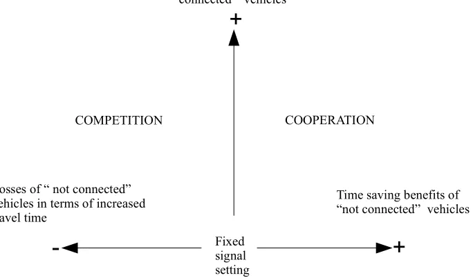
An evaluation of FCDATS systems in terms of competition-cooperation is proposed which is based on the dual utility diagram proposed by M. Cipolla [46] which assigns an action to four quadrants depending if the action brings benefits or losses to others or to themselves. Since in FCDATS systems there are only two group of drivers which can benefit (or loose) in terms of travel time gains (or losses) such a diagram seems able to capture the level of cooperation-competition.
Since it presents level of competition and cooperation at the same time we will call this diagram "Coopetition diagram". The diagram is structured as shown in the following Figure 1. The x axis is the percentage gain or loss in term of average travel time, with respect to a non controlled situation, for "not connected" vehicles while the y axis is the percentage of gain for "connected" vehicles.
Figure 1. Coopetition (competition-cooperation) diagram.
FCDATS systems regulates traffic lights according to the known position of some percentage of total vehicles. The traffic signal regulation algorithms would tend to minimize queuing and delays at intersections. To obtain this result it is useful to know the queue length for every group of lanes that is coupled with a turning manoeuvre. In the case of intersections with a single lane for each incoming road the accuracy of smart-phone GNSS data is usually enough to establish the length of the queue and apply queue based control algorithms. Instead in the case of multiple lanes this is cannot be given for granted.
Time saving benefits of “connected” vehicles
+
+
Fixedsignal setting
-Losses of “ not connected” vehicles in terms of increased travel time
Time saving benefits of “not connected” vehicles COOPERATION
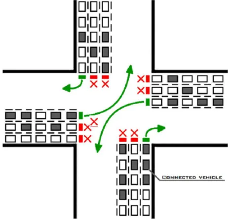
As an example, in a situation such as that depicted in Figure 2, FCDATS systems would be more accurate to reduce traffic delays at intersection by knowing the exact lane distribution of instrumented vehicles (dark shaded vehicles) in queues.
The accuracy of GNSS smart-phone data has become the object of research in [47], in a study on the reconstruction of traffic light cycles from FCD data. The GPS position was compared to the simulated one and an error area was used, with a radius given from a normal distribution with average 0 and standard deviation 25 m. This hypothesis derives from [48] in which the GPS position was corrected with Bayesian filters using data from different sensors. However, the study was intended for pedestrian GPS position correction and not vehicles. Speeds were, in fact between 0 and 2 m/s.
Figure 2. An example of signalized intersection, where, exact lane position information would be useful for FCDATL systems.
Prior to these studies Angermann [49] also hypothesized that the position of GPS data would be replicated through a normal distribution with accuracy parameter between 20 and 30 meters. In other studies conducted on GPS signal reception problems [15],[50][51][52][53][54] it was found out that in environment where there are buildings and direct occlusions to satellite tracking the error increases. GNSS can fail among tall buildings in situations that are defined as “urban canyons”. The need to recognize the lane occupancy of a car is also useful in autonomous driving. In this case cameras are used to detect the lane markings. An overview of the state-of-the-art of camera techniques can be found in [55]. Algorithms have been developed to correct satellite data and obtain an accurate positioning on the road e.g. in: [56] or [57] . The problem in most GNSS car positioning systems is that the accuracy is not enough to identify lane occupancy. Solutions have been proposed to bring the accuracy to a level that would allow lane identification: [58] and [59] used for example differential GPS (D-GPS). Recent works on lane determination are: [60] and [61]. In [62] it is proposed a simple method for smartphone GPS to determine the lane position of a car.
In [63] a fuzzy set-based method, is proposed, for car positioning within road lanes near intersections using GPS data coming from smartphones. Fuzzy sets are used to take into account uncertainty embedded in GPS data trying to identify the position of cars within the road lanes. The proposed method was applied to three intersections in the urban road network of Bari (Italy). First results reveal the effectiveness of the proposed methodology when comparing the actual car lane positions and those determined by the method.
correlated to a number of factors such as the occlusion of the sky. The study produced a first algorithm to be inserted into micro simulators in order to correctly simulate FCD data.
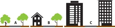
Experiments were made in three different scenarios. Figure 3 shows the three types of scenarios in which experimental data were gathered.
Case A represents a scenario where the satellite localization is almost perfect as the sky is almost completely visible. Case B represents a scenario where sight disturbances can reduce satellite signals. Case C is a scenario where there are tall buildings at least 18 meters on the side of the street (urban canyon). The experimental survey was conducted in the urban area of Cosenza (Italy) fully representing the three above described scenarios. A high precision GPS system was used to assess the accuracy of five different smart-phones in the three mentioned scenarios. In accordance with GNSS localization theory Rayleigh distribution was used as a reference for distance error and uniform distribution for angle error. Based on these experimental data a procedure was developed to reproduce GNSS error in traffic simulations and applied in this work.
Figure 3. Three scenarios for the experimental works of [64].
To evaluate performances of FCDATS systems we developed a special laboratory prototype in which to carry on experimental tests. Our laboratory prototype (Figure 4) is composed of a central server which is able to regulate traffic signal from connected vehicles data (such as one that can be used in real time on the field connected with real traffic signals) and another computer that creates a virtual reality environment making it possible to evaluate the performances of the proposed system before a real implementation on the field.
Figure 4. Traffic signal algorithms testing lab.
The virtual reality environment is created, with a micro-simulation module based on the Tritone microscopic traffic simulator [65][66].
The localization errors are generated in a dedicated module for post-processing of vehicles trajectories. This module is very important in correctly assessing performances of a traffic settings algorithm.
This is done addressing separately distance error (which is a positive variable theoretically distributed as a Rayleigh variable) and angle error (which follows a uniform distribution). Distance error, is generated, according to one of the three case scenarios, with a different Rayleigh distribution.
After the first time step, the error in distance is generated following a normal distribution with mean and standard deviation that are relative to one of the three scenarios and also relative to the error absolute value in the preceding time step (this is an empirical procedure that introduces some approximation). The experimental data showed, in fact, that autocorrelation translates into a different standard deviation of the error at time t+1 depending on the absolute value of the error at time t.
A similar procedure is carried out for the angle simulation where instead the autocorrelation can be reproduced by just using a normal distribution for each of the three scenarios fully in accordance with theory. This can be done exactly following theory since the angle distribution, not considering autocorrelation, is a simple uniform distribution.
The procedure above described is useful to generate a sequence of distance and angle errors and allows applying microsimulation to test generic ITS algorithms and strategies that are based on FCD data.
Generated Positions data are transferred via internet protocol to the central signal regulating server. The central server of the system elaborates positions, by correcting introduced random localization errors with a map-matching algorithm. Elaborated position data are then fed into the adaptive traffic signal algorithm (FCDATS).
To carry out the above described simulations, the GNSS error generation module, the map-matching algorithm and the algorithm for traffic light control were implemented using the microscopic traffic simulation model Tritone [67]. The use of TRITONE allowed automatic simulation of 20 repetitions for every scenario.
Inside Tritone specific car-following, emission and fuel consumption models were used as described in this section.
Car-following: one of the major concerns for considering signalization at intersections is the modelling of rear-end interactions involving vehicles travelling along the approaches. Approaching a slower leading vehicle (car-following regime) the driver must recognizes consciously some action points, and considers others unconsciously. The conscious actions depends on the speed difference, relative distance to the leading vehicle, and driver-depended behaviour. The Car-following Model that was selected to represent the interactions among vehicles of the traffic stream is Wiedemann 99 [68]. This model calculates the vehicle speed as the minimum of a speed based on the vehicle acceleration restrictions and another speed based on a steady-state car-following model. The model considers a vehicle kinematics model with a linear speed-acceleration relationship and allows the user to modify the desired and maximum driver speed-acceleration relationship. In TRITONE, the car-following model parameters are setted up according to [69], that calibrated Wiedemann 99 model in an urban intersection located in Southern Italy.
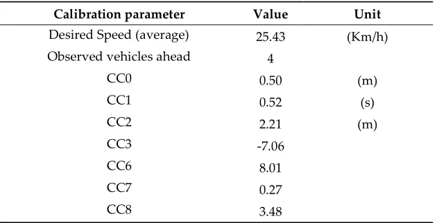
In their study, Gallelli et al. established that the parameters influencing significantly driver behaviour are: "Desired Speed" (average) (Km/h) that represents individual free flow speed, "Observed vehicle ahead" that influences drivers’ ability to adjust their speed/distance according to a given number of lead vehicles, "Standstill distance" (m) (CC0) that defines the desired distance between stopped cars, "Headway time" (s) (CC1), "Following variation" (m) (CC2) threshold for the entering “following” (CC3), "Positive following” threshold (CC5)," Speed dependency of oscillation" (CC6), "Oscillation acceleration" (CC7) and "Standstill acceleration" (CC8). The parameters values considered in TRITONE are reported in the following Table 1.
traffic and with traffic control in the same network. For all pollutant emission it was considered a general function which takes into account instantaneous speed and acceleration of vehicles. The pollutants modelled are nitrogen oxides (NOx), volatile organic compounds (VOC), carbon dioxide (CO2) and particulate matter (PM). This choice is based on their potential health impacts and external costs.
Table 1. Car following parameters..
Calibration parameter Value Unit
Desired Speed (average) 25.43 (Km/h) Observed vehicles ahead 4
CC0 0.50 (m)
CC1 0.52 (s)
CC2 2.21 (m)
CC3 -7.06
CC6 8.01
CC7 0.27
CC8 3.48
Fuel consumption model: The fuel consumption model considered is the Akcelik model [71]. The choice is due to highly accurate fuel consumption estimates for traffic analysis and the absence of any aggregation (simplification) in terms of traffic information (i.e average travel speed, average running speed and number of stops).
The vehicle parameters used in the fuel consumption model include fuel type (% diesel), maximum engine power, power to weight ratio, number of wheels and tyre diameter, rolling resistance factor, frontal area and the aerodynamic drag coefficient.
Fuel consumption is calculated for each of the four-mode elemental (modal) travelling cases: cruise, acceleration, deceleration and idling.
3. Results
A case study is presented where a simple greedy algorithm (more extensively described in [43]) is applied for the optimization of traffic settings based on FCD data. The algorithm establishes in real time the phase sequence, the green times and the total cycle time. It is based on the evaluation of the number of "connected" vehicles that are detected on every approaching street at the intersection. The algorithm at every cycle establishes the sequence of phases by choosing first the phases with more "connected" vehicles. Every phase receives a green time which is enough to clear the queue of "connected" vehicles. Vehicles that are not "connected" are not considered and the signal setting may change before some of them are able to exit the intersection. If there is no "connected" vehicle on some of the approaches the algorithm falls back on a reference pre-established cycle establishing green times according to the pre-established fixed times of green. In any case the algorithm assigns a minimum green of 4 seconds for every phase (according to traffic light UK rules). It must be noted that this simple algorithm can be used only on intersections that have one single lane for every approach.
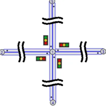
In this case study the simulated intersection is a typical symmetrical intersection with four approaching roads. Three different flow distributions were provided assuming that one direction is the main traffic direction: 60/40, 70/30 and 80/20. Approaching road links are of 200 meters each. The direction of links 2-3 and 3-2 (see Figure 5) is considered the main direction. The distribution, of the various manoeuvres for a single approach, is uniform with 1/3 of the vehicles turning left, right or proceeding straight.
Figure 5.Simulated road intersection
For the traffic demand a distribution such as that of the HCM 2010 [72] for the distribution of average daily traffic in urban areas is used. The distribution (Figure 6) was then approximated in order to obtain only four daily flows, 680, 424, 278 and 93 v / h.
Figure 6. Daily flow for local route
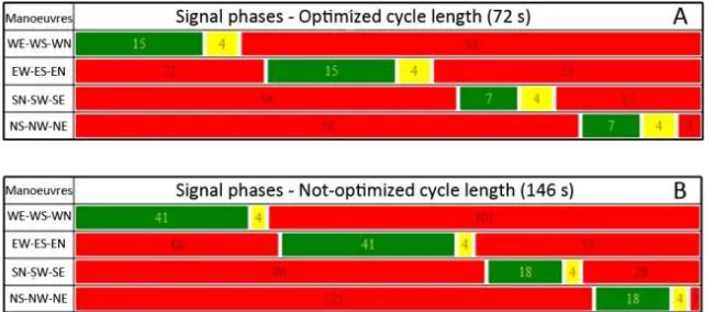
Figure 7. Traffic light cycle A and B
The static traffic light setting A was established, according to the HCM 2010 methodology, for peak traffic and a 70/30 distribution of flows, while the second setting B is the optimum for the same configuration but with double total traffic. The B signal setting variant was created to evaluate the hypothesis in which the traffic light system is badly regulated, in the first place, to better assess how the FCD-based algorithm system automatically works to improve the way green are established.
A preliminary analysis was carried out based on the evaluation of the Ratio of Travel Time Saving (RTTS) both for “connected” and “not connected” vehicles expressed as follows:
𝑅𝑇𝑇𝑆 = ( ), (1)
𝑅𝑇𝑇𝑆 = ( ), (2)
in which:
RTTSC is the Ratio of Travel Time Saving for “connected” vehicles; RTTSNC is the Ratio of Travel Time Saving for “not-connected” vehicles;
TTO is the overall average travel time of the intersection four entry links (including service time) assuming that no vehicles are “connected” (no regulation of the traffic signal is applied);
RTTSC is the Ratio of Travel Time Saving for “connected” vehicles;
TTC(p) is the average travel time of the “connected” vehicles of the entry links of the intersection
(including service time) assuming that penetration rate of “connected” vehicles is p.
Simulations were performed by varying the percentage of “connected” vehicles, also to establish which is, for this specific scenario, the minimum number of “connected” vehicles needed to have an optimal regulation. For this reason the same scenario has been replicated by simulating different percentages of “connected” vehicles from 5% to 100% in increments of 5%.
3.1 Competition-cooperation diagrams
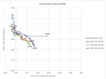
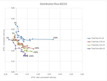
In the following Figures 8,9,10 and 11 some results in terms of "coopetition" diagram (above defined) are presented. Four different values of total flow and three different directional distributions have been considered for cases A and B (20 repetitions of each scenario were performed) for each percentage of "connected" vehicles (21 different cases) for a total number of 10.080 simulations (20 repetitions of each scenario were performed).
For brevity sake only results relative to a directional flow distribution 60/40 and 80/20 are presented in Figures 8,9,10 and 11 for case A and case B. Results show that the FCDATS systems impacts always positively on Travel Time Saving of "connected" vehicles especially in case B where confrontation is carried on in a bad regulated intersection.
Figure 8. Ratio of Travel Time Saving for traffic light cycle A (Distribution of flow 60/40)
Figure 9. Ratio of Travel Time Saving for traffic light cycle B (Distribution of flow 60/40)
Figure 10. Ratio of Travel Time Saving for traffic light cycle A (Distribution of flow 80/20)
Figure 11. Ratio of Travel Time Saving for traffic light cycle B (Distribution of flow 80/20)
competition between "connected" vehicles and "not connected" vehicles", "connected" vehicles are taking green time away from "not connected" vehicles" and the points in the "coopetition" diagram are on the left of the y axis. This disadvantage for "not connected" vehicles disappears when more vehicles become "connected". The marginal utility of the “not-connected” vehicles increases for all simulated scenarios with an increase of "connected" vehicles".
On the other hand, when basic traffic light cycle is bad regulated, in the first place (traffic light cycle B), “not-connected” vehicles benefit from an improvement in travel times even in the presence of very low percentages of “connected vehicles” both for balanced distributions and for unbalanced distributions of traffic volumes on the main and the secondary directions (Figures 9 and 11). Overall, we can observe a better optimization of travel times through the proposed FCDATS compared to static-flows based regulated traffic light cycles (i.e. traffic light cycle A).
It should be noted that FCDATS advantages seems to decrease with the increase of total flow. In most cases (also with flow distribution 70/30 which is not in presented in the figures) the curves in the "coopetition" diagram shift left and down when the intersection is more saturated (total flow increasing). The only exception we found in our simulation is in the case A with a 60/40 distribution of flow.
3.2 Average results of a typical day
Results based on averaging the simulation for a typical day are based on the distribution of total flows of Figure 6 as in Table 2:
Table 2. Distribution of daily flow. Flow
veh/h Hours
93 6
278 6 424 8 680 4
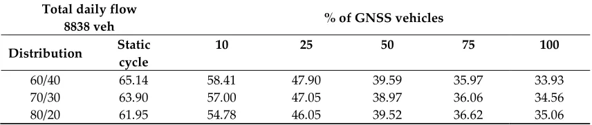
The following Tables 3 and 4 show the average travel time for case A and B:
Table 3. Average travel time [sec.], in a typical day, for case A. Total daily flow
8838 veh % of GNSS vehicles
Distribution Static Cycle 10 25 50 75 100
60/40 47.42 46.60 42.97 38.44 36.06 34.29 70/30 46.25 45.13 42.78 38.18 36.06 34.88 80/20 45.30 44.39 41.88 38.05 36.79 35.70
Table 4. Average travel time [sec.] in a typical day for case B: bad regulated intersection. Total daily flow
8838 veh % of GNSS vehicles
Distribution Static cycle 10 25 50 75 100
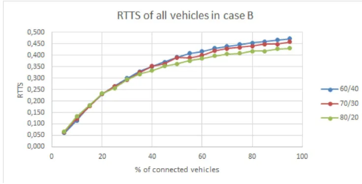
Results of table 3 and 4 are also presented in Figures 12 and 13 in terms of RTTS for all vehicles as a function of percentage of "connected" vehicles.
Figure 12. RTTS for all vehicles in case A
Figure 13. RTTS for all vehicles in case B
Tables 5 and 6 show the average values of fuel consumption for case A and B:
Table 5. Average fuel consumption [liters/km], in a typical day, for case A. Total daily flow
8838 veh % of GNSS vehicles
Distribution Static cycle 10 25 50 75 100
Table 6. Average fuel consumption [liters/km], in a typical day, for case B. Total daily flow
8838 veh % of GNSS vehicles
Distribution Static cycle 10 25 50 75 100
60/40 0.276 0.257 0.229 0.209 0.201 0.198 70/30 0.280 0.259 0.232 0.213 0.204 0.201 80/20 0.276 0.257 0.234 0.217 0.211 0.208
Tables 7 and 8 show the average values of CO2 pollution:
Table 7. Average CO2 pollution [g/km], in a typical day, for case A. Total daily flow
8838 veh % of GNSS vehicles
Distribution Static Cycle 10 25 50 75 100
60/40 89.946 89.373 85.875 82.111 81.424 79.695 70/30 91.566 90.957 87.793 84.334 83.212 81.402 80/20 94.134 93.077 90.909 87.834 86.957 85.177
Table 8. Average CO2 pollution [g/km], in a typical day, for case B. Total daily flow
8838 veh % of GNSS vehicles
Distribution Static Cycle 10 25 50 75 100
60/40 102.795 97.619 89.392 82.127 80.126 79.161 70/30 106.503 99.765 91.211 85.744 82.035 80.865 80/20 107.129 101.319 93.110 87.532 85.710 84.160
FCDATS show a general reduction of travel times, fuel consumption and pollutant emissions in all scenarios compared with values obtained from static signal regulation. The tables from 3 to 10 show that FCDATS perform better in case A than in case B in terms of absolute values when the percentage of "connected" vehicles is equal or less than 50%. This happens since the initial conditions are different. The algorithm in case A is based on a better calculated static reference signal cycle. The algorithm in cases where there are no "connected" vehicles, at the intersection, falls back on this basic static reference cycle and this means that in the scenarios of case B sometime the wrong static reference signal cycle is applied bringing higher travel times and lower performances. This problem disappears when the percentage of connected vehicles is 75% or 100% since there would be fewer situations where the algorithm cannot rely on "connected" vehicles to adjust signal phases.
Improvements of FCDATS with respect to the static cycle derive mainly from the reduction of travel time on the links entering the intersection, but also from the reduced number of stop-and-go events near the traffic light, which consequently reduces the number of sudden braking and deceleration/acceleration.
The overall results compared to the static reference signal cycle are positive in all cases showing that FCDATS system can be implemented with benefit in all situations. The expected performances are to a larger extent better at intersections where the static signal cycle is not well established.
Table 9. Average NOx pollution [g/km], in a typical day, for case A. Total daily flow
8838 veh % of GNSS vehicles
Distribution Static Cycle 10 25 50 75 100
60/40 1.152 1.147 1.092 1.026 0.999 0.977 70/30 1.159 1.156 1.113 1.047 1.020 1.004 80/20 1.189 1.176 1.144 1.080 1.062 1.040
Table 10. Average NOx pollution [g/km], in a typical day, for case B. Total daily flow
8838 veh % of GNSS vehicles
Distribution Static Cycle 10 25 50 75 100
60/40 1.422 1.322 1.168 1.051 0.997 0.973 70/30 1.431 1.322 1.175 1.070 1.018 1.000 80/20 1.437 1.336 1.206 1.102 1.065 1.041
And finally tables 11 and 12 show the average values of PM pollution in a typical day:
Table 11. Average PM pollution [g/km], in a typical day, for case A. Total daily flow
8838 veh % of GNSS vehicles
Distribution Static cycle 10 25 50 75 100
60/40 0.013 0.012 0.012 0.011 0.011 0.011 70/30 0.013 0.013 0.012 0.012 0.012 0.012 80/20 0.014 0.014 0.013 0.013 0.013 0.013
Table 12. Average PM pollution [g/km], in a typical day, for case B. Total daily flow
8838 veh % of GNSS vehicles
Distribution Static cycle 10 25 50 75 100
60/40 0.014 0.013 0.012 0.011 0.011 0.011 70/30 0.014 0.013 0.012 0.012 0.012 0.012 80/20 0.015 0.014 0.013 0.013 0.013 0.012
3.3Average results of a typical day in terms of competition-cooperation
of "connected" vehicles. Connected vehicles are obtaining better travel times on a daily average at the expense of not "connected" vehicles. When the percentage of "connected" vehicles goes over 30% in all cases the effects of competition disappear since RTTS becomes positive also for not "connected" vehicles.
Figure 13. Competition-Cooperation diagram on a daily base in case A
Results for the intersection which is starting from a bad signal cycle are instead always positive also for not "connected" vehicles, RTTS is always positive for both categories of vehicles as shown in Figure 14.
4. Discussion
The paper gives a first assessment of the penetration rate of "instrumented" vehicles that is necessary in order to obtain a good real time regulation in a FCDATS system and on the meaning of competition-cooperation in such a system.
A dedicated microsimulation lab was developed specifically to test FCDATS algorithm. The choice of microsimulation to test algorithms has a long historical background: traffic signal regulation has been verified and evaluated in simulation since the well-known Webster formula for delays which was evaluated in 1966 with the first computer traffic simulations.
Results of the simulations show a good performance of the simple implemented greedy algorithm even with a low percentage of "instrumented" vehicles.
All performance measures, in terms of average travel time, fuel consumption and pollutant emissions, were improving compared to the values of the original static signal cycle. Some level of competition among different classes of vehicles was revealed in some of the scenarios. Vehicles which are not "connected" may suffer disadvantages in terms of travel time with traffic regulation from FCDATS, for the benefit of "connected" vehicles, especially when the percentage of connected vehicles and the total flow at intersection are low.
Results evaluated in terms of fuel consumption and pollutant emissions prove that FCDATS systems can be an effective new solution, among smart city innovations, to increase transportation sustainability.
The algorithm used in the simulation was a simple greedy algorithm allowing other researchers to reproduce results. It has the shortcoming of using a reference pre-established regulation cycle which is applied when there are no "connected" vehicles at the intersection. The algorithm could be improved in such a way that it would not be necessary to fall back on a static reference cycle. This can be done in many different ways. In situations where there are no "connected" vehicles a more complicated algorithm could use a reference cycle, which is calculated on an average estimated percentage of "connected" vehicles such as the ψ ratio of instrumented vehicles to the total traffic flow applied in [11]. Also Kalman filtering could be applied to obtain a good estimation of the needed green times when there are no "connected" vehicles. Future research efforts can be dedicated to develop specific algorithms to apply in specific cases.
The algorithm presented in this paper represents the first approach to analyze the traffic light regulation of a four legs intersection using FCDATS. More complicated intersections would need different and more complicated algorithms. Future research can also be devoted to find more general optimization algorithms that would perform a good regulation in general cases.
Genetic algorithms may be candidate for a better solution of the problem given the complications involved that do not allow a simple analytical representation.
5. Conclusions
The competition between "connected" vehicles and not "connected" vehicles is a real problem which could hold back the use of innovative traffic signal regulation systems based on Floating Car Data. This paper has shown that for a simple four legs intersection the disadvantages for not "connected" vehicles are less than the total advantages for the community.
Figure 15. Ratio of performances (compared with static signal cycle) for case A.
Author Contributions: V.A. was responsible for conceptualization and methodology, V.P.G. carried on the computer lab implementations, G.G. and A.V. performed supervision, review and editing.
Funding: This research received no external funding.
Conflicts of Interest: The authors declare no conflict of interest.
References
1. Vittorio, A.; Demetrio Carmine, F.; Vincenzo Pasquale, G. Cooperative-competitive paradigm in traffic signal synchronization based on floating car data. In International Conference on Environment and Electrical Engineering and 2018 IEEE Industrial and Commercial Power Systems Europe (EEEIC/I&CPS Europe); 2018.
2. Schubert, R.; Schlingelhof, M.; Cramer, H.; Wanielik, G. Accurate positioning for vehicular safety applications - The SAFESPOT approach. In IEEE Vehicular Technology Conference; 2007.
3. Benmimoun, M.; Zlocki, A.; Eckstein, L. Advanced Driver Assistance Systems: Benefit Evaluation Method and User Acceptance for Adaptive Cruise Control and Collision Warning System. Transp. Res. Board 91st … 2012.
4. Stahlmann, R.; Festag, a; Tomatis, a; Radusch, I.; Fischer, F. Starting European Field Tests for Car-2-X Communication : the Drive C2X Framework. ITS World 2011.
5. Jahangiri, A.; Rakha, H.; Dingus, T. A. Red-light running violation prediction using observational and simulator data. Accid. Anal. Prev. 2016, doi:10.1016/j.aap.2016.06.009.
6. Cassini Martin NO IDLE MATTER: How signal-controlled traffic could be doing more harm than good. TRAFFIC Technol. Int. 2007, 56.
7. Steve Huntingford Traffic lights cause more harm than good Available online: https://www.telegraph.co.uk/cars/comment/traffic-lights-cause-more-harm-than-good/ (accessed on Oct 12, 2018).
9. Cassini, M. In your car no one can hear you scream! Are traffic controls in cities a necessary evil? Econ. Aff. 2006, doi:10.1111/j.1468-0270.2006.00675.x.
10. Astarita, V.; Florian, M. The use of mobile phones in traffic management and control. ITSC 2001. 2001 IEEE Intell. Transp. Syst. Proc. (Cat. No.01TH8585) 2001, doi:10.1109/ITSC.2001.948621.
11. Astarita, V.; Bertini, R. L.; d’Elia, S.; Guido, G. Motorway traffic parameter estimation from mobile phone counts. Eur. J. Oper. Res. 2006, 175, doi:10.1016/j.ejor.2005.02.020.
12. Barceló, J.; Montero, L.; Marqués, L.; Carmona, C. Travel Time Forecasting and Dynamic Origin-Destination Estimation for Freeways Based on Bluetooth Traffic Monitoring. Transp. Res. Rec. J. Transp. Res. Board 2010, doi:10.3141/2175-03.
13. Barceló, J.; Montero, L.; Bullejos, M.; Serch, O.; Carmona, C. A kalman filter approach for exploiting bluetooth traffic data when estimating time-dependent od matrices. J. Intell. Transp. Syst. Technol. Planning, Oper. 2013, doi:10.1080/15472450.2013.764793.
14. Guido, G.; Vitale, A.; Saccomanno, F. F.; Festa, D. C.; Astarita, V.; Rogano, D.; Gallelli, V. Using Smartphones as a Tool to Capture Road Traffic Attributes. Appl. Mech. Mater. 2013, doi:10.4028/www.scientific.net/AMM.432.513.
15. Guido, G.; Gallelli, V.; Saccomanno, F.; Vitale, A.; Rogano, D.; Festa, D. Treating uncertainty in the estimation of speed from smartphone traffic probes. Transp. Res. Part C Emerg. Technol. 2014, doi:10.1016/j.trc.2014.07.003.
16. Herrera, J. C.; Work, D. B.; Herring, R.; Ban, X. (Jeff); Jacobson, Q.; Bayen, A. M. Evaluation of traffic data obtained via GPS-enabled mobile phones: The Mobile Century field experiment. Transp. Res. Part C Emerg. Technol. 2010, doi:10.1016/j.trc.2009.10.006.
17. Chen, W. J.; Chen, C. H.; Lin, B. Y.; Lo, C. C. A traffic information prediction system based on Global Position System-equipped probe car reporting. Adv. Sci. Lett. 2012, doi:10.1166/asl.2012.2192.
18. Zhou, X.; Wang, W.; Yu, L.; Zhou, X.; Yu, Á. L.; Wang, W.; Lu, W. Traffic Flow Analysis and Prediction Based on GPS Data of Floating Cars. In Lecture Notes in Electrical Engineering; 2012.
19. Guido, G.; Vitale, A.; Astarita, V.; Saccomanno, F.; Giofré, V. P.; Gallelli, V. Estimation of Safety Performance Measures from Smartphone Sensors. Procedia - Soc. Behav. Sci. 2012, doi:10.1016/j.sbspro.2012.09.824.
20. Bierlaire, M.; Chen, J.; Newman, J. P. Modeling Route Choice Behavior From Smartphone GPS data. Transport 2010.
21. Händel, P.; Ohlsson, J.; Ohlsson, M.; Skog, I.; Nygren, E. Smartphone-based measurement systems for road vehicle traffic monitoring and usage-based insurance. IEEE Syst. J. 2014, doi:10.1109/JSYST.2013.2292721.
22. Astarita, V.; Caruso, M. V.; Danieli, G.; Festa, D. C.; Giofrè, V. P.; Iuele, T.; Vaiana, R. A Mobile Application for Road Surface Quality Control: UNIquALroad. Procedia - Soc. Behav. Sci. 2012, doi:10.1016/j.sbspro.2012.09.828.
23. Vaiana, R.; Iuele, T.; Astarita, V.; Caruso, M. V.; Tassitani, A.; Zaffino, C.; Giofrè, V. P. Driving behavior and traffic safety: An acceleration-based safety evaluation procedure for smartphones. Mod. Appl. Sci. 2014, 8, doi:10.5539/mas.v8n1p88.
24. Astarita, V.; Guido, G.; Mongelli, D.; Giofrè, V. P. A co-operative methodology to estimate car fuel consumption by using smartphone sensors. Transport 2015, 30, doi:10.3846/16484142.2015.1081280. 25. Gap Analysis in Cooperative Systems within Intelligent Transportation Systems, Royal Institute of
26. Newell, G. F. TRAFFIC SIGNAL SYNCHRONIZATION FOR HIGH FLOWS ON A TWO-WAY STREET. Itte Calif Univ Res. Reports 1967.
27. Bavarez, E.; Newell, G. F. Traffic Signal Synchronization on a One-Way Street. Transp. Sci. 1967, 1, 55–73, doi:10.1287/trsc.1.2.55.
28. Hillier, J. a.; Rothery, R. The Synchronization of Traffic Signals for Minimum Delay. Transp. Sci. 1967. 29. Gartner, N. OPTIMAL SYNCHRONIZATION OF TRAFFIC SIGNAL NETWORKS BY DYNAMIC
PROGRAMMING. Traffic Flow Transp. 1972.
30. Sims, A. G.; Dobinson, K. W. The Sydney Coordinated Adaptive Traffic (SCAT) System Philosophy and Benefits. IEEE Trans. Veh. Technol. 1980, doi:10.1109/T-VT.1980.23833.
31. Robertson, D. I.; Bretherton, R. D. Optimizing Networks of Traffic Signals in Real Time—The SCOOT Method. IEEE Trans. Veh. Technol. 1991, doi:10.1109/25.69966.
32. Sehgal, V. K.; Dhope, S.; Goel, P.; Chaudhry, J. S.; Sood, P. An embedded platform for intelligent traffic control. In Proceedings - UKSim 4th European Modelling Symposium on Computer Modelling and Simulation, EMS2010; 2010.
33. Faye, S.; Chaudet, C.; Demeure, I. Multiple intersections adaptive traffic lights control using a wireless sensor networks Contrôle adaptatif des feux de circulation sur de multiples intersections à l’aide d’un réseau de capteurs sans fil Département Informatique et Réseaux Multiple Intersections Adaptive Traffic Lights Control using a Wireless Sensor Networks; 2013;
34. Clempner, J. B.; Poznyak, A. S. Modeling the multi-traffic signal-control synchronization: A Markov chains game theory approach. Eng. Appl. Artif. Intell. 2015, doi:10.1016/j.engappai.2015.04.009.
35. Ilal Ghazal, B.; Eikhatib, K. Smart Traffic Light Control System. In 2016 Third International Conference on Electrical, Electronics, Computer Engineering and their Applications (EECEA); 2016.
36. Al-Khateeb, K.; Johari, J. A. Y. Intelligent dynamic traffic light sequence using RFID. IEEE Int. Conf. Comput. Commun. Eng. 2008 2008, doi:10.1109/ICCCE.2008.4580829.
37. Sharma, S.; Pithora, A.; Gupta, G.; Goel, M.; Sinha, M. Traffic Light Priority Control For Emergency Vehicle Using RFID. Int. J. Innov. Eng. Technol. 2013, 2, 363–366.
38. Neumann, T. A Cost-Effective Method for the Detection of Queue Lengths at Traffic Lights. In Traffic Data Collection and its Standardization ; Springer, New York, NY, 2010; pp. 151–160.
39. Kerper, M.; Wewetzer, C.; Sasse, A.; Mauve, M. Learning traffic light phase schedules from velocity profiles in the cloud. In 2012 5th International Conference on New Technologies, Mobility and Security - Proceedings of NTMS 2012 Conference and Workshops; 2012.
40. Axer, S.; Friedrich, B. Level of service estimation based on low-frequency floating car data. In Transportation Research Procedia; 2014.
41. Axer, S.; Friedrich, B. Estimating signal phase and timing for traffic actuated intersections based on low frequency floating car data. In IEEE Conference on Intelligent Transportation Systems, Proceedings, ITSC; 2016.
42. J., G. Traffic Technology International. 2016, pp. 52–54.
43. Astarita, V.; Giofrè, V. P.; Guido, G.; Vitale, A. The use of adaptive traffic signal systems based on floating car data. Wirel. Commun. Mob. Comput. 2017, 2017, doi:10.1155/2017/4617451.
44. Competition Available online: https://en.wikipedia.org/wiki/Competition. 45. Cooperation Available online: https://en.wikipedia.org/wiki/Cooperation. 46. Cipolla, C. M. Allegro ma non troppo; Il Mulino, 1988; ISBN 978-88-15-01980-6.
based on low frequency floating car data. In Proceedings of the 6th mobility TUM (2015); 2015.
48. Wendlandt, K.; Khider, M.; Angermann, M.; Robertson, P. Continuous location and direction estimation with multiple sensors using particle filtering. In 2006 IEEE International Conference on Multisensor Fusion and Integration for Intelligent Systems; 2006.
49. Angermann, M.; Kammann, J.; Robertson, P.; Steingaß, A. Software representation for heterogeneous location data sources using probability density functions. In International Symposium on Location Based Services for Cellular Users (LOCELLUS 2001).; 2011.
50. Ochieng, W. .; Sauer, K. Urban road transport navigation: performance of the global positioning system after selective availability. Transp. Res. Part C Emerg. Technol. 2002, doi:10.1016/S0968-090X(02)00008-6. 51. Wang, B. Application of Smartphone for Intersection Performance Measurement, University of Akron,
Civil Engineering., 2011.
52. Zandbergen, P. A. Accuracy of iPhone locations: A comparison of assisted GPS, WiFi and cellular positioning. In Transactions in GIS; 2009.
53. Zandbergen, P. A.; Barbeau, S. J. Positional accuracy of assisted GPS data from high-sensitivity GPS-enabled mobile phones. J. Navig. 2011, doi:10.1017/S0373463311000051.
54. Zhang, J.; Li, B.; Dempster, A. G.; Rizos, C. Evaluation of High Sensitivity GPS Receivers. In 2010 International Symposium on GPS/GNSS; Taipei, Taiwan. , 2010.
55. Bar Hillel, A.; Lerner, R.; Levi, D.; Raz, G. Recent progress in road and lane detection: A survey. Mach. Vis. Appl. 2014.
56. Zhao, X. On processing GPS tracking data of spatio-temporal car movements: a case study. J. Locat. Based Serv. 2015, doi:10.1080/17489725.2015.1098738.
57. Fouque, C.; Bonnifait, P. Matching raw GPS measurements on a navigable map without computing a global position. IEEE Trans. Intell. Transp. Syst. 2012, doi:10.1109/TITS.2012.2186295.
58. Farrell, J.; Givargis, T. Differential GPS reference station algorithm - design and analysis. IEEE Trans. Control Syst. Technol. 2000, doi:10.1109/87.845882.
59. Du, J. D. J.; Barth, M. Bayesian Probabilistic Vehicle Lane Matching for Link-Level In-Vehicle Navigation. 2006 IEEE Intell. Veh. Symp. 2006, doi:10.1109/IVS.2006.1689681.
60. Moon, S.-C.; Kim, B.-S.; Kim, J.-J.; Lee, S.-G. Discrimination of Traffic Lane Departure Based on GIS Using DGPS. In 17th ITS World Congress, Busan, 2010: Proceedings; Busan , Korea, South, 2010.
61. Basnayake, C.; Lachapelle, G.; Bancroft, J. Relative Positioning for Vehicle-to-Vehicle Communications-Enabled Vehicle Safety Applications. In 18th ITS World Congress; Orlando Florida, United States, 2011.
62. Sekimoto, Y.; Matsubayashi, Y.; Yamada, H.; Imai, R.; Usui, T.; Kanasugi, H. Lightweight lane positioning of vehicles using a smartphone GPS by monitoring the distance from the center line. In IEEE Conference on Intelligent Transportation Systems, Proceedings, ITSC; 2012.
63. Marinelli, M.; Palmisano, G.; Astarita, V.; Ottomanelli, M.; Dell’Orco, M. A Fuzzy set-based method to identify the car position in a road lane at intersections by smartphone GPS data. In Transportation Research Procedia; 2017; Vol. 27.
64. Giofre, V. P.; Astarita, V.; Guido, G.; Vitale, A. Localization issues in the use of ITS. In 5th IEEE International Conference on Models and Technologies for Intelligent Transportation Systems, MT-ITS 2017 - Proceedings; 2017.
66. Guido, G.; Astarita, V.; Giofré, V.; Vitale, A. Safety performance measures: A comparison between microsimulation and observational data. In Procedia - Social and Behavioral Sciences; 2011; Vol. 20, pp. 217–225.
67. Giofrè, V. P.; Maciejewski, M.; Merkisz-Guranowska, A.; Piątkowski, B.; Astarita, V. Real road network application of a new microsimulation tool: TRITONE. Arch. Transp. 2013, 27–28.
68. PTV PTV Planung Transport Verkehr. (VISSIM User Manual Version 7.0) 2014.
69. Gallelli, V.; Iuele, T.; Vaiana, R.; Vitale, A. Investigating the transferability of calibrated microsimulation parameters for operational performance analysis in roundabouts. J. Adv. Transp. 2017, 2017, doi:10.1155/2017/3078063.
70. Int Panis, L.; Broekx, S.; Liu, R. Modelling instantaneous traffic emission and the influence of traffic speed limits. Sci. Total Environ. 2006, doi:10.1016/j.scitotenv.2006.08.017.
71. Akcelik, R. Progress in Fuel Consumption Modelling for Urban Traffic Management. Publ. Aust. Road Res. Board 1983, doi:0 86910 123 4.