Optimisation in NZ electricity market

Dr Bhujanga B. Chakrabarti, SM IEEE

Academic Staff Member

Wintec Institute of Technology

IIT, Kharagpur February 5, 2019

Overview of Presentation

• NZ Power System

– Power Systems – Renewables

– Load, LDC and Load curves – Generation mix

– Energy mix

• NZ Electricity Market

– Major characteristics

– Different Dispatch Schedules

– Security Constrained Dispatch Model

• Market Clearing Engine (SPD)

– SPD in NZEM

– LMP and issues in SPD – Risk-Reserve

– Modelling of Branch Loss – Transmission Congestion – Relieving Congestion

• Simultaneous Feasibility Test (SFT)

– New Market System (June 2009) – AC and DC SFT

NZ Power System and Electricity Market

• Operated by Transpower as Independent S.O

• North & South islands with HVDC interlink (1200 MW)

• 220, 110 and 66 kV AC and 350 kV DC

• 400 kV OH Transmission coming soon this year

• Main bodies: Transpower , Electricity Authority and Commerce Commission

• LMP market, ½ hourly trading periods

• More than 700 market nodes in the MCE (SPD-LP)

• Thermal constraints generated by ACSFT and SPD

• Energy and Operating reserve co-optimized every

5 minute (Not FK regulating reserve)

• Open Access to transmission

• Unit commitment: Generators are self committed

• FTR, DSP, and Scarcity price are coming soon

• 11800KM,HVAC +250KM 400kV, 180 SS, 4100

Renewable Resources in New Zealand

• NZ Government mandate is to have 90 % of our electricity generated from renewable resources by 2025.

• We generated just over ¾ th of our electricity by renewable resources in 2011.

• We expect more than 1000 MW renewable resources will be added during this period. Major part of it is expected to be Wind

Wind Power, Existing World Capacity, 1996–2010

Installed Generation Mix in NZ Market - 2011

GAS + GT CO_GEN THERMAL CCGT WIND GEO-THERMAL HYDRO

Total = 9645 MW

• Independent System Operator

• LMP (locational marginal pricing) based dispatch

• Generators are self committed

• Transparent constraint management

• Open access to transmission

• Co-ordinated ancillary services

• Market based pricing

• Market power mitigation

• Mandatory system security standards

New Zealand

Electricity

Market (NZEM)

Major Characteristics…..contd

Market Place

• Sellers (Gens)

• Buyers (Consumers)

• Service Providers (Transpower, LINE COs)

• Market Operators SO, Transpower

Major characteristics …contd

• NZEM is the first among the 2nd _{generation LMP Electricity Markets.}

Operated since OCT 01, 1996

• It is a LMP market

• Energy and operating reserves and FRR are co-optimised. That means both energy and reserves could compete for the same

Major Characteristics…..contd

• Unit commitment: Generators are self committed.

• Gate closure occurs 1hrs before actual real time dispatch .

• In US, ISOs use different UCs for procuring capacities in DAM, HAM, RTM.

• Offers and Bids: Generators offer

– energy bids ($/MWH) in upto 10 blocks (steps)

– Reserve bids for both 6s and 60s reserves in upto 3 steps

• Demanders also bid for their load ($/MWH). Demand bids are used only in one schedule (PRSS). Other schedules use forecasted

Major Characteristics…..contd

• Network Losses are modeled inside SPD, approximating quadratic

loss function as linear loss segments ( 1 or 3 or 6 segments depending upon the type of network element).

• Static loss of each branch is modeled as load equally at each end.

• Dynamic loss for each branch is modeled at the receiving end only.

Major Characteristics…..contd

• NZEM does not intervene to minimise network Congestion. The

effect of congestion is reflected in the nodal price. However we monitor the degree of congestion, by Lerner Type price ratios. • In US, ISOs manage congestion using bids, and using injection

sensitivities

• We do not mitigate Market Power. The market is still is not very

clear in defining possession , exercising Market power at this stage. We got a report from Professor Frank Wollak of University of

California, examined whether Market players in NZ (gens) exercised market power using 10 years market data. YES.

Different Dispatch Schedules

The following schedules run in parallel but with different periodicity. Some schedules have variable intervals. Periodicity include Daily, 2hr, 1/2hr and 5 minute. Runs like train of pulses.

• Weekly Daily Schedule (WDS)

– Runs Daily.

– Uses SFT Build Thermal constraints.

• NRSS (Non-price Responsive Schedule Small)

– Runs every 1/2 hr, mainly for security check. – Output is secured dispatch.

– Uses forecast demand.

– Uses SFT Build Thermal constraints.

• PRSS (Price Responsive Schedule Small)

– Runs every 1/2hr.

Different Dispatch Schedules

• NRSL similar to NRSS but every 2 hrs, Covers Longer Period.

• PRSL similar to PRSS but every 2 hrs, Covers Longer Period.

• RTD (Real time dispatch)

– Runs every 5 minute.

– Load is calculated internally from the 1st RTD run : The final 2nd run calculates, Load = System generation-Losses recorded in Pass 1. This load is distributed among areas and buses using predefined Load distribution factors(LDFs).

– Uses Thermal constraints from NRSS

• RTP (Real time pricing)

– Run every 5 minutes – Uses ST Load forecast.

Different Dispatch Schedules

• FP (Final Pricing)

– Runs every ½ hour, next day

– Market is settled on these Final prices. – It uses Metered load.

– Constraints from recent NRSS schedules

• Find

Optimal generation and reserve dispatch, and Nodal spot prices

• To minimise

Dispatch (energy and reserve) cost

• Subject to

▪ Meet demand at each “bus” (= node)

▪ Meet energy and reserve offers

▪ Meet power balance at each bus

▪ Meet line capacity and other limit constraints

▪ Meet N-1 Security and other Security constraints

▪ Meet unit risk reserve requirements

Security Constrained Dispatch

SPD in NZEM

SPD is a security constrained DC-OPF based application (works on Linear Program method).

Bus Injections

AC & DC Branch Flows

Branch Losses

Branch Flow Constraints

Bus Power Balance Constraints

Bus Group Generation MW

Market Node Group Constraints

Mixed Constraints

Ramping Constraints

Risk-Reserve constraints

N-1 Thermal constraints

Stability constraints

Power System Normal Operation Control

• One of the most important power system control objectives is to keep the

balance in the system.

• At any moment, at any bus, the generation must meet load + Losses, and

net line flows. Power balance at each bus(node) is used as opposed to a single system wide power balance equation, as used in ISOs.

• In US, ISOs use three processes that achieve this goal under normal operations: automatic generation control (AGC), load following, and

optimal/economic dispatch.

• In NZ, we now balance the system through 5min dispatch and with FRR.

How are Nodal Prices (LMPs) calculated?

• Marginal cost is the cost of next MW, – the Marginal generator is the generator that

would be dispatched to supply the next MW, (assuming unconstrained dispatch-only one marginal generator)

• A nodal price is the cost of serving the next MW of load at a given location

• Nodal prices are derived by solving a “dual” problem of a primal security constrained

dispatch problem.

• Nodal prices consists of 3 components:

Nodal Price Marginal cost of

generation

= +

Marginal cost of Transmission

Congestion

Marginal cost of

LMP Components

• Energy Component – Marginal generation price.

• Loss Component - is the marginal cost of additional losses caused by supplying an increment of load at the location.

US ISOs: System-Wide Power Balance

• This constraint says that total generation in the system should balance the load plus the transmission losses.

• There is only one system wide PB constraint and this is an equality constraint and thus always binding.

• The dual variable associated with this constraint is the System-Energy price.

T

t

En

En

En

En

L load t load G unit t

unit

−



=

+





;

T

t

En

En

En

=

+



;



)

.(

)

.(

L load t node t base unit t unit G unit t node t

loss

En

En

En

En

En

=

−

−

−







 

Issues in SPD

• Multiple solutions

• Degeneracy

• Non-physical loss due to CBF and Loss trench swapping

• Infeasibility: To handle problem of infeasibility under certain circumstances, violation variables for constraints with upper/lower limits are added and additional terms of penalizing the violation variables are added to objective function

• Surplus Branch Flow, Deficit (Surplus) Bus Generation, Deficit (Surplus) Branch Group Flow Constraint,Deficit (Surplus) Bus Group Generation Constraint, Deficit (Surplus) Market Node Constraints, Deficit (Surplus) Mixed Constraint, Deficit 6 Second Reserve

Reserve Modelling in NZEM

•

Generator Risk

; ,

Cleared Generation of Risk generator, u

Cleared Reserve of Risk generator, u

= Total requirement of reserve from all generators R P R u u Risk units

i u u i

P u

R u

R i i

 _{ +  }

=

=

Reserve constraints

• Proportional constraint

• Reserve upper bound constraint

• Generator joint capacity constraint

• Generator upper and lower bound constraint

i i

i

x

P

R



.

max i i

R

R



i

R

P

P

+



Reserve Model

• Operating or Contingency Reserves

• 6 Second reserve (needs to be activated within 6s and must last minimum 60s) • 60 Second reserve(needs to be activated within 60s and must last minimum 15

minutes)

• Who supplies reserves?

• On-line resources (generators)

• Interruptible Loads (should be activated within 1s and must remain disconnected for 60s or 15 minutes).

• How do the reserve providers bid and paid?

• How do the reserve providers bid and how are they paid?

• Providers can bid for the same capacity into Energy, 6s and 60s reserve markets simultaneously as per their capability

• Market may clear all or some or none products depending on the requirements, bid prices and the maximum capacity of the resource.

• Reserve providers are paid for availability, and also for energy provided during the interval, if called for.

• How do we control Frequency?

• We use AGC.

• Co-optimised through bidding

• Requirements of FR reserves are set by user.

Reserve Requirements

• We need contingency (operating) reserves to cover the generator / HVDC

pole outage risks. Usually it is the outage of the largest operating generator or HVDC pole outage (N-1).

• The reserves are 6s reserve and 60s reserve –used to contain the system

frequency at 48Hz (for N-1) in 6s, and at the pre-disturbance value in 60s. We are allowed to shed limited load, over and above reserves, for N-2 generator contingency.

• We used to calculate requirement of reserves in advance, by a tool called

RMT. We replaced it by special module added with TSAT. These requirements are passed on to the SPD.

• We also calculate the “stand-by residual check” outside the SPD to make

sure that the available offers for reserves are adequate to manage the 2nd

gen contingency while the 1st _{one is still on. It is not a constraint within the}

Ramp Up/Down

• Generators offer for both ramp up/down rate per hour and their limits (for

energy only, now). The effect of binding ramp constraints are reflected in the nodal prices, and also in dispatches.

• Different schedules calculate the ramp MW according to their duration and

the rate.

1

( ) : ; ( ( , ) ). 2

L

ij ij i j ij ij ij

P = B  − + P   i j L

N_i All nodes connected to bus i.

P_di Demand at bus i.

P_gi Generation at bus i.

Bij Line susceptance between i and j in pu.

R_ij Resistance of the line, in pu.

θ_i Bus voltage angle at bus I,in radian.

.

2

; ( , )

.

L

ij ij ij ij

P

=

R P



i j



L

Branch Loss

Branch Loss Model



.

is the dual variable associated with the energy balance equality constraint at

each bus i. It represents the Locational Marginal Energy Price at the bus i. It

captures:

• The marginal generation cost

• The marginal cost of loss

• The marginal cost of network congestion, and

• The shadow prices of other binding constraints

i



Nodal Energy Balance Constraint _{gi di ij}

:

;

.

j Ni

P

P

P



i



Linear Loss Model: 3 Seg Branch Loss

1 2

1

2

2 2 2 2

1 2 1 1 1

0

2 2 2 3 [ ] [ ( ) ] [ ( ) ] . R P P P P R R P

LSE m x Rx dx m x P Rx m P dx

m x P Rx RP dx

= − + − − + +

− − +







X0 P1 P2 PR Powerflow Y0 Y A xi s Y3 Y2

Y1 ΔX3

ΔY3 L os se s X Axis Break

Points(X) Loss (Y)

m = (Y_k-Y_k-1) /(Xk-Xk-1)

P0 0 0

P1 0.3101021 0.072129

0.23259762 3

P2 0.6898979 0.452097

1.00045314 6

P3 1 1

Advantages of Linear Loss model

• Formulation is linear and can be solved using Linear programming method

• MIP can be added to break the loss tranches from lower to higher tranches, in this order, on top of the LP solution without loss of accuracy.

• Break points P₁ and P₂ are linear functions of the ratings P_R, and the marginal loss

(gradients) m₁, m₂ and m₃ are functions of R and P_R.

• Thus these constants can be calculated off-line for transmission off-lines and transformers

1 2 1 2 3 (4 6 5 (1 6 5

3(4 6 11) 10( 6 4)

.

(3 6 28) 20 R R R R R P P P P m RP

m R P

Disadvantages of Linear Loss Model

• The approach will tend to produce flows at the corner points of the loss tranches.

• Marginal loss is step-wise linear approximation of the real linear marginal loss function. Thus this approximation has much greater pricing impact than the absolute error in the loss.

• Number of loss tranches should be greater enough to ensure greater accuracy.

• Non-Physical Loss

Non-Physical (NP) Loss

• The model assumes that the problem is entirely separable i.e. each loss tranche is a separate decision variable and there is no in-built logic to force them to be taken in flow order (adjacency conditions). • Normally the optimization will minimize the losses and thus the low

loss tranche will be used first before using the higher loss tranches. • BUT, Constraints, Negative gen offer → SPD Tends to maximize →

Negative Nodal prices (locally/system wide).

• Optimization then prefers to maximize the losses near the node and will choose the highest loss tranches first. Addl losses are known as NP Losses.

• A solution with non-physical loss usually exhibit one or both of the following symptoms:

– Directional flow variables are chosen for both forward and backward flow directions simultaneously.

Loss Coefficients A= 0. 3101; C = 0. 14495 D= 0. 32247; E = 0. 46742

F= 0. 82247

Branch Segments

Br Segment Flow limit (1 ) = 10000.

Br Segment Loss Factor (1) = 0.01 *100 Rpu* BR MW

capacity.

Segments = 1

Br Segment Flow limit (1 ) = BR MW capacity* Coef_A. Br Segment Loss Factor (1) = 0.01 *100 Rpu* BR MW

capacity* 0. 75* Coef_A. Br Segment Flow limit (2 ) = BR MW capacity*(1- Coef_A ).

Br Segment Loss Factor (2) = 0.01 *100 Rpu* BR MW

capacity.

Br Segment Flow limit (3 ) = 10000.

Br Segment Loss Factor (3) = 0.01 *100 Rpu* BR MW capacity*(2-0. 75* Coef_A ).

Segments = 3

Br Segment Flow limit (1 ) = BR MW capacity* Coef_ C. Br Segment Loss Factor (1) = 0.01 *100 Rpu* BR MW

capacity* 0. 75* Coef_ C. Br Segment Flow limit (2 ) =

BR MW capacity* Coef_ D. Br Segment Loss Factor (2) = 0.01 *100 Rpu* BR MW

capacity*. Coef_E. Br Segment Flow limit (3 ) = 0.5* BR MW capacity. Br Segment Loss Factor (3) = 0.01 *100 Rpu* BR MW

capacity* Coef_ F. Br Segment Flow limit (4 ) = BR MW capacity*(1- Coef_ D ).

Br Segment Loss Factor (4) = 0.01 *100 Rpu* BR MW

capacity*(2- Coef_ F). Br Segment Flow limit (5 ) = BR MW capacity*(1- Coef_ C ).

Br Segment Loss Factor (5) = 0.01 *100 Rpu* BR MW

capacity*(2- Coef_E ). Br Segment Flow limit (6 ) =

10000.

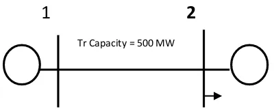
Effect of Transmission Congestion

- Two node network with no loss. See Figure A2.

Figure A2: Two node loss less network

Tr Capacity = 500 MW

1 2

Gen 1 Capacity = 1000 MW Marginal cost MC1 = $20/ MWH

Congestion Rent = 15,000

p2=50

p1=20

500 600

a

b

c

d f

e

h g

MW Load

Price

No transmission Congestion

Spot price (system marginal price) at node 1 & 2 ₁ = ₂ = $20 / MWH. Total generation cost = area “abde” = 600 *20= $12000

Total bill paid by the customer = area “abde” = 600*20 = 12,000

With Transmission Congestion for a transmission capacity = 500 MW

Since transmission line is congested, a marginal electricity demand at node 2 can be met only by using expensive power generated at node 2.

Marginal price at node 2, ₂= 50 /MWH.

How does it look like in P1-P2 plane?

We consider now PTDF, SF1 at bus = 1 and that at

bus SF2 =0

250 2 ). 4 ( 1000 1 ). 3 ( 500 1 2 . 2 1 . 1 ). 2 ( 600 2 1 ). 1 ( : 2 50 1 20 :    = + = + + = P P P P SF P SF P P ST P P Min OBJ

The constraint in

P1-P2 plane looks like:

Total cost (20P1+50P2) at (500,100) =$15000

(350,250) =$19500

Relieving Congestion in ISOs

• Base case is available

• Suppose circuit 1-2 is overloaded by 47 MW in a 3 gen and 5 bus system. Swing = G1.

• That means we need to reduce flow in this circuit by 47 MW by re-dispatching in order to bring back its flow to its limit.

New Market System (2009)

Major new components are

• CSM (Common Source Modeler) • MOI (Market Operator Interface)

• SFT Simultaneous Feasibility Test (Full AC) • MDB (Main data base)

• SPD’s mathematical model remains same but rewritten to

accommodate changes in the input and the output of other MSP components.

• e-node (electrical node), and P-node (Pricing node has been

Modes of Operation in SFT

• Topper

• AC SFT and Non-linear DC SFT (Back up)

• SFT Check

• VSAT

Input-Output in New Market System

• Integrated market system operates in real time, and talks with its different components to help managing and operating the system.

• Also, some components can be operated in Stand Alone mode (SPD, SFT).

• In S/A mode, both the SPD, and SFT communicates with the user through

csv flies. The SPD and SFT also creates csv files. Some examples of csv files to/from SPD are:

• Input files to SPD

– MDBCTRL csv file →type of schedule, input files etc – Static Network file

– Dynamic network file – Period file

– Market file – MOD file

• Output files from SPD

SPD-SFT Iterations

• The network, offers, load bids, load forecast, initial set of constraints, and different limits are made available to SPD. SPD calculates optimal dispatch (and nodal prices) and passes to SFT.

• SFT also receives additional data for reactive load, voltage profile, and capacitor switching schedule through the data base.

• SFT recalculates the set of thermal constraints based on contingency violations, and these are passed to SPD to produce a feasible and secure dispatch.

• The iteration between SPD and SFT continues

– until solution convergence occurs, or

AC SFT Constraint Formulation

• SFT is based on Fast Decoupled Load Flow method (Alsac and Scott)

• Gets Network from Topper, MW dispatch from SPD, Reactive load, voltage Schedule and Capacitor switching schedule from MDB, and set of Contingencies

• Performs Load flow, Contingency Analysis, Sensitivity Analysis

Branch Flow PDF and Thermal Constraint

P

P

DF

P

−

=

Distribution factor of Flow in P when C Out

Power Flow in P during post-contingency

Power Flow in P during pre-contingency

Power Flow in C during pre-contingency

Coefficient due to thermal char of conductor DFpc ' Pp Pp Pc

1 P pc

.

k P

+

DF P



Rating

1

k Thermal Constraint

Benefits of using SFT

– SFT uses up-to-date network and injection data for developing constraints, and is therefore providing optimal application of security constraints

– All possible contingencies are considered automatically.

– The process is automated removing a considerable manual burden with attendant risks.

Challenges of using SFT

• Convergence in AC Load flow

– Load flow non-convergence could occur, but not expected very frequently from the operating network

• Non-Convergence/Infeasibility in the SPD

• Non-Converge in Cascaded SPD-SFT loop

• Convergence is monitored based on max{Change in generation dispatch over all nodes, from SPD, between any two successive iterations (del Pg} <= a set threshold

• OR , terminated after a maximum number of iterations (user defined)

Minimise cost for each interval

The model’s objective is to minimise the total generation costs over 24 hourly intervals(1).

The load at bus 8 (WH schedule) must be met by wind, hydro and if necessary by thermal generations (3).

The constraints (4, 5) express the forward and reverse flow of each branch.

Power balance at each bus must be respected (6).

Demand is set at each bus (7). ;

Acknowledgements

Speaker would like to acknowledge:

• Mr Kieran Devine, GM, SO Transpower NZ Ltd, and

End of Presentation