Article
On near optimality of one-sample update for joint
detection and estimation
Yang Cao1, Liyan Xie1, Yao Xie1*, Huan Xu1
1 H. Milton Stewart School of Industrial and Systems Engineering, Georgia Institute of Technology; {caoyang,
lxie49}@gatech.edu, {yao.xie, huan.xu}@isye.gatech.edu * Correspondence: [email protected]
Abstract:Sequential hypothesis test and change-point detection when the distribution parameters
1
are unknown is a fundamental problem in statistics and machine learning. We show that for such
2
problems, detection procedures based on sequential likelihood ratios with simple one-sample update
3
estimates such as online mirror descent are nearly second-order optimal. This means that the upper
4
bound for the algorithm performance meets the lower bound asymptotically up to a log-log factor in
5
the false-alarm rate when it tends to zero. This is a blessing, since although the generalized likelihood
6
ratio(GLR) statistics are optimal theoretically, but they cannot be computed recursively, and their exact
7
computation usually requires infinite memory of historical data. We prove the nearly second-order
8
optimality by making a connection between sequential analysis and online convex optimization and
9
leveraging the logarithmic regret bound property of online mirror descent algorithm. Numerical and
10
real data examples validate our theory.
11
Keywords: sequentialmethods; change-pointdetection; onlinealgorithms
12
1. Introduction
13
Sequential analysis is a classic topic in statistics concerningonlineinference from a sequence of
14
observations. The goal is to make statistical inferenceas quickly as possible, while controlling the false
15
alarm rate. Two related sequential analysis problems commonly studied are sequential hypothesis
16
testing and sequential change-point detection [1]. They arise from various applications including
17
online anomaly detection, statistical quality control, biosurveillance, financial arbitrage detection and
18
network security monitoring (see, e.g., [2,3]).
19
We are interested in joint estimation and detection in sequential analysis, which occurs when
20
there are unknown parameters for data distribution. For instance, in change-point detection, given a
21
sequence of samplesX1,X2, . . ., a common assumption is that they are i.i.d. with certain distribution
22
fθparameterized byθ, and the values ofθare different before and after the change-point. One can
23
assume that before the change, the parameter value isθ0. This is reasonable since, in various settings,
24
there is a relatively large amount of background data. Thus, the parameterθin the normal state can be
25
estimated with good accuracy. After the change, the value of the parameter switches to anunknown
26
value, and it represents an anomaly or novelty that needs to be discovered.
27
1.1. Motivation: Dilemma of CUSUM and generalized likelihood ratio (GLR) statistics
28
Consider change-point detection with unknown parameters. A commonly used change-point
29
detection method is the so-called CUSUM procedure [3]. It can be derived from likelihood ratios.
30
Assume that before the change, the samples Xifollow a distribution fθ0, and after the change, the
31
samplesXi follow another distribution fθ1. CUSUM procedure has a recursive structure. Initiate
32
with W0 = 0. The likelihood-ratio statistic can be computed according to Wt+1 = max{Wt+
33
log(fθ1(Xt+1)/fθ0(Xt+1)), 0}, and a change-point is detected wheneverWt exceeds a pre-specified
34
threshold. Due to the recursive structure, CUSUM ismemory efficient, since it does not need to store the
35
historical data and only needs to record the value ofWt. However, one possible issue with CUSUM is
36
the choice of the post-change parameterθ1. In practice, it is usually chosen to represent the “smallest”
37
change-of-interest. However, this choice is somewhat subjective. In the multi-dimensional setting, it
38
is hard to define what the “smallest” change would mean. Moreover, when the assume parameter
39
θ1deviates significantly from the true parameter value, CUSUM may suffer a severe performance
40
degradation [4].
41
An alternative approach is the Generalized Likelihood Ratio (GLR) statistic [5]. The GLR statistic
42
finds the maximum likelihood estimate (MLE) of the post-change parameter and plugs it back
43
to the likelihood ratio to form the detection statistic. To be more precise, for each hypothetical
44
change-point locationk, the corresponding post-change samples are {Xk+1, . . . ,Xt}. Using these
45
samples, one can form the MLE denoted as ˆθk,t. Without knowing whether the change occurs and
46
where it occurs beforehand when forming the GLR statistic, we have to maximizekover all possible
47
change locations. The GLR statistic is given by maxk<t∑ti=k+1log(fθˆk,t(Xi)/fθ0(Xt)), and a change
48
is announced whenever it exceeds a pre-specified threshold. The GLR statistic is more robust than
49
CUSUM [6], and it is particularly useful when the post-change parameter may vary from one situation
50
to another. However, a drawback of GLR statistic is that it isnot memory efficientand it cannot be
51
computed recursively. Moreover, when there is a constraint on the maximum likelihood estimator
52
(such as sparsity), MLE cannot have closed-form solution; one has to store the historical data, and
53
re-estimates ˆθk,t whenever there is new data. As a remedy, the window-limited GLR is usually
54
considered, where one only keeps the pastwsamples, and restrict the maximization overkto be over
55
(t−w,t]. However, even with window-limited GLR, one still has to re-estimate ˆθk,tusing historical
56
data whenever the new data are added.
57
In practice, rather than CUSUM or GLR, various one-sample update schemes are used especially
58
in machine learning literature. The one-sample update schemes perform online estimates of the
59
unknown parameter, and plug the estimates into the likelihood ratio statistic to perform detection.
60
The one-sample update takes the form of ˆθt=h(Xt, ˆθt−1)for some functionhthat uses only the most
61
recent data and the previous estimate. Some examples of one-sample estimate schemes include online
62
gradient descent and online mirror descent (similar scheme has been used in [7,8]). The one-sample
63
update enjoys efficient computation, as the information from the new data can be incorporated via low
64
computational cost update such as mirror descent, which even has closed-form solution in some cases.
65
It is also memory efficient since the update only needs the most recent sample. Such estimator may
66
not correspond to the exact MLE, but they tend to have good performance. An important question
67
remains to be answered:how much performance do we lose by using one-sample update schemes rather than
68
the exact GLR?
69
1.2. Application scenario: Social network change-point detection
70
The widespread use of social networks (such as Twitter) leads to a large amount of user-generated
71
data generated continuously. One important aspect is to detect change points in streaming social
72
network data. These change points may represent the collective anticipation of or response to external
73
events or system “shocks” [9]. Detecting such changes can provide a better understanding of patterns
74
of social life. In social networks, a common form of the data is discrete events over continuous time. As
75
a simplification, each event contains a time label and a user label in the network. In our prior work [10],
76
we model discrete events data using network point processes, which capture the influence between
77
users through aninfluence matrix. We then cast the problem as detecting changes in influence matrix.
78
We assume that the influence matrix in the normal state (before the change) can be estimated from the
79
reference data. After the change, the influence matrix is unknown since it’s due to an anomaly, and
80
it has to be estimated online. Due to computational burden and memory constraint, since the scale
of the network can be large, we do not want to store the entire historical data and rather compute
82
the statistic in real-time. In [10], we develop a one-sample update scheme to estimate the influence
83
matrix and then form the likelihood ratio detection statistic. However, theoretical performance of such
84
one-sample update schemes has not been well-understood.
85
1.3. Contributions
86
This paper aims to address the above question by proving the nearly second-order optimality of
87
simple one-sample update schemes for sequential hypothesis test and change-point detection. The
88
nearly second-order optimality [3] means that the upper bound for performance matches the lower
89
bound up to a log-log factor. In particular, we consider likelihood ratios with plug-in online mirror
90
descent estimator. Our approach generalizes the non-anticipating estimator framework [11] from
91
detecting Gaussian mean shift to the exponential family with constrained parameters. Here we focus
92
on online mirror-descent, but the result can be generalized to other schemes such as the online gradient
93
descent. The proof leverages the logarithmic regret property of online mirror descent and the lower
94
bound established in statistical sequential analysis literature [3,12]. Synthetic examples validate the
95
performances of one sample update schemes.
96
The contributions of the paper are summarized as follows
97
• We provide a general upper bound for sequential hypothesis test and change-point detection
98
procedures with the one-sample update schemes. The upper bound explicitly captures the impact
99
of estimation on detection by anestimation algorithm dependentfactor. This factor shows up as an
100
additional term in the upper bound for the expected detection delay, and it corresponds to the
101
regret bound of the estimator. This establishes an interesting linkage betweensequential analysis
102
andonline convex optimization1.
103
• Using our upper bound and existing lower bound, we show that the one-sample update schemes
104
are nearly second-order optimal for the exponential family. Moreover, numerical examples
105
verify the good performance of one-sample update schemes. They can perform better and are
106
more robust than the likelihood ratio methods with pre-specified parameters (e.g., CUSUM
107
for change-point detection). Moreover, they are computationally efficient alternatives of GLR
108
statistic (which requires storing infinite samples) and cause little performance loss relative to
109
GLR.
110
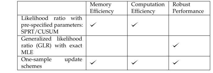
The comparison of three approaches is summarized in Table1.
111
Table 1.Comparison of three approaches. Memory
Efficiency
Computation Efficiency
Robust Performance Likelihood ratio with
pre-specified parameters: SPRT/CUSUM
Generalized likelihood ratio (GLR) with exact MLE
One-sample update schemes
1.4. Literature and related work
112
Sequential analysis is a classic subject with an extensive literature. Much success has been
113
achieved when the pre-change and post-change distributions are exactly specified. For example, the
114
CUSUM procedure [15] with first-order asymptotic optimality [16] and exact optimality [17] in the
115
minimax sense, the Shiryayev-Roberts (SR) procedure [18], which can be derived based on a Bayesian
116
principle and it enjoys various optimality. Both CUSUM and SR procedures rely on likelihood ratios
117
between the specified pre-change and post-change distributions.
118
The GLR [6,19] statistic enjoys certain optimality properties, but it can not be computed
119
recursively in most cases [43]. To address the infinite memory issue, [6,20] studied the
120
window-limited GLR procedure. Another approach aiming to address the issue is called the
121
Shiryayev-Roberts-Robbins-Siegmund (SRRS) procedure [11]. The main idea of SRRS dates back
122
to the power one sequential test [21]: instead of plugging in the MLE obtained using all samples
123
up to the current moment as done in the GLR procedure, the SRRS procedure uses a sequence of
124
non-anticipating estimators. The non-anticipating estimators are formed by dropping the most recent
125
sample (thus the name “non-anticipating”). The advantage is that the test statistic can be computed
126
recursively. However, there is a small loss of performance which can be bounded. The original
127
SRRS procedure [21] was developed for Gaussian when the post-change mean is unknown. Our
128
work extends it to the general exponential family via the adaptive SRRS (ASR) procedure. Our
129
non-anticipating estimator is also different from the original SRRS [21] in that SRRS still uses exact
130
MLE estimated from all but the most recent sample, whereas our estimator only approximates the
131
MLE using one-sample update schemes.
132
With unknown parameters, [22] developed a modified SR procedure by introducing a prior
133
distribution to the unknown parameters; however, the resulted detection statistic is hard to compute
134
recursively since the prior is not a conjugate. The more recent work [23] and [24] study joint detection
135
and estimation problem of a specific form: a linear scalar observation model with Gaussian noise,
136
and under the alternative hypothesis there isan unknown multiplicative parameter. This problem arises
137
from many applications such as spectrum sensing [25], image observations [26], MIMO radar [27], etc.
138
[23] demonstrates that solving the joint problem by treating detection and estimation separately with
139
the corresponding optimal procedure does not yield an overall optimum performance, and provides
140
an elegant closed-form optimal detector. Later on [24] generalizes the results. There are also other
141
approaches solving the joint detection-estimation problem using multiple hypotheses testing [26,28]
142
and Bayesian formulation [29]. Our work differs from the above in that we consider the general form
143
of joint detection and estimation problem, where the unknown parameterθshows up generally as
144
the parameter of the exponential family. Moreover, we do not aim to find the exact optimal solution.
145
Instead, we find whether using the computationally efficient one-sample estimator for detection loses
146
much performance.
147
Related work using online convex optimization for anomaly detection include [7], which develops
148
an efficient detector for the exponential family using online mirror descent and proves a logarithmic
149
regret bound, and [8], which dynamically adjusts the detection threshold to allow feedbacks about
150
whether decision outcome. However, these works consider a different setting that the change is a
151
transient outlier instead of a persistent change, as assumed by the classic statistical change-point
152
detection literature. When there is persistent change, it is important to accumulate “evidence” by
153
pooling the post-change samples (our work considers the persistent change).
154
Extensive work has been done for parameter estimation in the online-setting. This includes
155
online density estimation over the exponential family by regret minimization [7,8,13], sequential
156
prediction of individual sequence with the logarithm loss [30,31], online prediction for time series
157
[32], and sequential NML (SNML) prediction [31] which achieves the optimal regret bound. Our
158
problem is different from the above, in that estimation is not the end goal; one only performs parameter
159
estimation to plug them back into the likelihood function for detection. Moreover, a subtle but
160
important difference of our work is that the loss function for online detecting estimation is−fθˆi(Xi),
whereas our loss function is−fθˆi−1(Xi)in order to retain themartingale property, which is essential to
162
establish the nearly second-order optimality.
163
On a high level, the problem of joint detection and estimation is also related to universal source
164
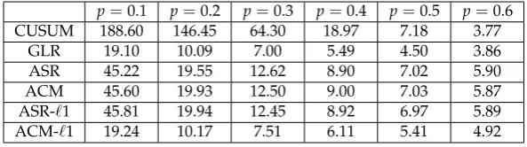
coding [33,34] or Minimum Description Length (MDL) [35,36]. In universal source coding, the goal is
165
to minimize the cumulative Kullback-Leibler (KL) loss.
166
2. Preliminaries
167
Assume a sequence of i.i.d. random variablesX1,X2, . . . with a probability density function of a
168
parametric form fθ. The parameterθmay be unknown. Consider two related problems: sequential
169
hypothesis test and sequential change-point detection. The detection statistic relies on a sequence
170
estimators {θˆt} constructed using online mirror descent. The online mirror descent uses simple
171
one-sample update: the update from ˆθt−1to ˆθtonly uses the current sampleXt. This is the main difference
172
from the traditional generalized likelihood ratio (GLR) statistic [6], where each ˆθtis estimated using
173
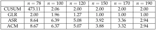
historical samples. In the following, we present detailed descriptions for two problems. We will
174
consider exponential family and present our non-anticipating estimator based on the one-sample
175
estimate.
176
2.1. Sequential hypothesis test
177
Consider null hypothesisH0 :θ =θ0versus the alternativeH1 :θ 6= θ0. Hence the parameter
under the alternative distribution is unknown. The classic approach to solve this problem is the sequential probablity-ratio test (SPRT) [37]: at each time, given samples{X1,X2, . . . ,Xt}, the decision
is either to acceptH0, acceptH1, or taking more samples if neithter hypotheses can be resolved
confidently. Here, we introducemodified SPRTwith a sequence ofnon-anticipatingplug-in estimators: ˆ
θt:=θtˆ(X1, . . . ,Xt), t=1, 2, . . . , (1)
Define the likelihood ratio at timetas
Λt=
t
∏
i=1
fθˆi−1(Xi) fθ0(Xi)
, i≥1. (2)
The test statistic has a simple recursive implementation
Λt=Λt−1· fθˆi−1(Xi)/fθ0(Xi).
Moreover, it has a martingale property due to the non-anticipating nature of the estimator:Efθ 0[Λt] = Efθ
0[Λt−1]. The decision rule is a stopping time
τ(b) =min{t≥1 : logΛt≥b}, (3)
whereb>0 is a pre-specified threshold. We reject the null hypothesis whenever the statistic exceeds
178
the threshold. The goal is to resolve the two hypotheses using as few samples as possible under the
179
type-I error constraint.
180
2.2. Sequential change-point detection
181
distribution of the data. One would like to detect such a change as quickly as possible. Formally, change-point detection can be cast into the following hypothesis test:
H0: X1,X2, . . . i.i.d.
∼ fθ0,
H1: X1, . . . ,Xνi.i.d.∼ fθ0, Xν+1,Xν+2, . . . i.i.d.
∼ fθ,
(4)
Here we assumeθis unknown, and it represents the anomaly. The goal is to detect the change as
182
quickly as possible after it occurs under the false alarm constraint.
183
We will consider likelihood ratio based detection procedures adapted from two types of existing
184
ones, which we call adaptive CUSUM (ACM), and the adaptive SRRS (ASR) procedures.
185
For change-point detection, the post-change parameter is estimated using post-change samples. This means that, for each putative change-point location before the current timek<t, the post-change samples are{Xk, . . . ,Xt}; with a slight abuse of notation, the post-change parameter is estimated as
ˆ
θk,i =θˆk,i(Xk, . . . ,Xi), i≥k. (5)
Therefore, fork=1, ˆθk,ibecomes ˆθidefined in (2) for SPRT. Base on this, the likelihood ratio at timet
for a hypothetical change-point locationkis given by
Λk,t= t
∏
i=k
fθˆk,i−1(Xi) fθ0(Xi)
, θˆk,k−1=θ0. (6)
whereΛk,tcan be computed recursively similar to (2).
186
Since we do not know the change-point locationν, from the maximum likelihood principle, we
take the maximum of the statistics over all possible values ofk. This gives the ACM procedure:
TACM(b) =inf
t≥1 : max
1≤k≤tlogΛk,t>b
, (7)
wherebis a pre-specified threshold.
187
Similarly, by replacing the maximization in (6) with summation, we obtain the following ASR procedure [11], which can be interpreted as a Bayesian statistic similar to the Shiryaev-Roberts procedure.
TASR(b) =inf
(
t≥1 : log
t
∑
k=1
Λk,t
!
>b
)
, (8)
wherebis a pre-specified threshold. The computations ofΛk,tand estimator{θtˆ},{θˆk,t}are discussed
188
later in section2.3.
189
2.3. Online mirror descent (OMD) for non-anticipating estimators
190
Next, we discuss how to construct the non-anticipating estimators{θtˆ}t≥1in (1), and{θˆk,t}, 1≤
191
k<tin (5) using online mirror descent (OMD). OMD is a generic procedure for solving the online
192
convex optimization problem (OCP). Our problem of finding maximum likelihood estimator can be
193
cast into an OCP with the loss function being the negative log-likelihood`t(θ):=−logfθ(Xt).
194
The main idea of OMD is the following. At each time step, the estimator ˆθt−1is updated using the
new sampleXt, by balancing the tendency to stay close to the previous estimate, against the tendency to move in the direction of the greatest local decrease of the loss function. For the loss function defined above, a sequence of OMD estimator is constructed by
ˆ
θt=arg min u∈Γ [u
|∇`
t(θtˆ−1) + 1 ηi
HereΓ ⊂ Θσ is a closed convex set, which is problem-specific and encourages certain parameter
195
structure such as sparsity. Similarly, ˆθk,tcan be constructed via OMD for sequential change-point
196
detection.
197
There is an equivalent form of OMD, presented as the original formulation in [42]. The equivalent
198
form is sometimes easier to use for algorithm development, and it consists of four steps: (1) compute
199
the dual variable: ˆµt−1 = ∇Φ(θˆt−1); (2) perform the dual update: ˆµt = µˆt−1−ηt∇`t(θˆt−1); (3)
200
compute the primal variable: ˜θt = (∇Φ)∗(µtˆ ); (4) perform the projected primal update: ˆθt =
201
arg minu∈ΓBΦ(u, ˜θt). The equivalence between the above form for OMD and the nonlinear projected
202
subgradient approach in (9) is proved in [41]. We adopt this approach when deriving our algorithm
203
and follow the same strategy as [7]. Our algorithm is presented in Algorithm1.
204
A standard performance metric for OCP isregret. The regret is the difference between the total cost that an online algorithm has incurred relatively to that of the best fixed decision in hindsight. Given samplesX1, . . . ,Xt, the regret for a sequence of estimators{θˆi}ti=1is defined as
Rt= t
∑
i=1
{−logfθˆi−1(Xi)} − inf ˜ θ∈Θ
t
∑
i=1
{−logfθ˜(Xi)}. (10)
For strongly convex loss function, the regret of many OCP algorithms, including the online mirror
205
descent, has the property thatRn≤Clognfor some constantC(depend onfθandΘσ) and any positive
206
integern [8,38]. Note that for exponential family, the loss function is the negative log-likelihood
207
function, which is strongly convex overΘσ. Hence, we have the logarithmic regret property.
208
2.4. Exponential family
209
In this paper, we focus onfθbeing the exponential family for the following reasons: (i) exponential
210
family [8] represents a very rich class of parametric and even many nonparametric statistical models
211
[39]; (ii) the negative log-likelihood function for exponential family−logfθ(x)is convex, and this
212
allows us to perform online convex optimization with nice theoretical properties. Some useful
213
properties of the exponential family are briefly summarized below, and full proofs can be found
214
in [8].
215
Consider an observation spaceX equipped with a sigma algebraBand a sigma finite measureH
on(X,B). Assume the number of parameters isd. Letx|denote the transpose of a vector or matrix. Letφ : X → Rdbe an H-measurable functionφ(x) = (φ1(x), . . . ,φd(x))|. Hereφ(x)corresponds
to the sufficient statistic forθ. LetΘdenote the parameter space inRd. Let{Pθ,θ ∈ Θ}be a set of
probability distributions with respect to the measureH. Then,{Pθ,θ∈Θ}is said to be a multivariate
exponential family with natural parameterθ, if the probability density function of each fθ ∈ Pθ
with respect toHcan be expressed as fθ(x) =exp{θ|φ(x)−Φ(θ)}. In the definition, the so-called
log-partition function is given by
Φ(θ):=log
Z
X exp(θ
|φ(x))dH(x).
To make sure fθ(x) a well-defined probability density, we consider the following two sets for
parameters:
Θ={θ∈Rd: log
Z
X exp(θ
|φ(x))dH(x)<+∞},
and
Θσ ={θ∈Θ:∇2Φ(θ)σId×d}.
Note that−logfθ(x)isσ-strongly convex overΘσ. Its gradient corresponds to∇Φ(θ) =Eθ[φ(X)],
and the Hessian∇2Φ(
θ)corresponds to the covariance matrix of the vectorφ(X). Due to this property,
Moreover,Φis aLegendre function, which means that it is strongly convex, continuous differentiable and essentially smooth [40]. The Legendre-Fenchel dualΦ∗is defined as
Φ∗(z) =sup
u∈Θ{u
|z−Φ(u)}.
The mappings∇Φ∗is an inverse mapping of∇Φ[41]. Moreover, ifΦis a strongly convex function, 216
then∇Φ∗= (∇Φ)−1.
217
A general measure of proximity used in online mirror descent is the so-calledBregman divergence BF, which is a nonnegative function induced by a Legendre functionF(see, e.g., [8,40]) defined as
BF(u,v):=F(u)−F(v)− h∇F(v),u−vi. (11)
For exponential family, a natural choice of the Bregman divergence is the Kullback-Leibler (KL) divergence. DefineEθas the expectation whenXis a random variable with density fθ, IntΘas be the
interior ofΘ, andI(θ1,θ2)as the KL divergence between two distributions with densities fθ1 andfθ2
for anyθ1,θ2∈Θ. Then
I(θ1,θ2) =Eθ1
log(fθ1(X)/fθ2(X))
. (12)
It can be shown that, for exponential family,I(θ1,θ2) =Φ(θ2)−Φ(θ1)−(θ2−θ1)|∇Φ(θ1). Using the
definition (11), this means thatBΦ
BΦ(θ1,θ2):=I(θ2,θ1)
is a Bregman divergence. This property is quite useful to constructing mirror descent estimator for the
218
exponential family [41,42].
219
Algorithm 1Online mirror-descent for maximum likelihood estimators
Require: Exponential family specificationsφ(x),Φ(x)and fθ(x); initial parameter valueθ0; sequence
of dataX1, . . . ,Xt, . . .; a closed, convex set for parameterΓ⊂Θσ; a decreasing sequence of strictly
positive step-sizes{ηt}. 1: θˆ0=θ0,Λ0=1. {Initialization}
2: for allt=1, 2, . . . ,do
3: Acquire a new observationXt
4: Compute loss`t(θˆt−1):=−logfθˆt−1(Xt) =Φ(θˆt−1)−θˆt|−1φ(Xt) 5: Compute likelihood ratioΛt=Λt−1×fθˆt−1(Xt)/fθ0(Xt) 6: µtˆ−1=∇Φ(θtˆ−1), ˆµt=µtˆ −1−ηt(µtˆ−1−φ(Xt)){Dual update} 7: θt˜ = (∇Φ)∗(µtˆ )
8: θtˆ =arg minu∈ΓBΦ(u, ˜θt){Projected primal update} 9: end for
10: return {θtˆ}t≥1and{Λt}t≥1.
3. Nearly second-order optimality of one-sample update procedures
220
Below we prove thenearly second-order optimalityof the one-sample update scheme based on
221
OMD. More precisely, the nearly second-order optimality means that the algorithm obtains the lower
222
performance bound asymptotically up to a log-log factor in the false-alarm rate, as the false alarm
223
rate tends to zero (In many cases the log-log factor is a small number). In particular, we show
224
that the performance ofτ(b)for sequential hypothesis testing,TACM(b)andTASR(b)for sequential
225
change-point detection setting, obtain the known lower bounds established in the statistical sequential
226
analysis literature up to a log-log factor.
227
We first introduce some necessary notations. DenotePθ,νandEθ,νthe probability measure and
228
expectation when the change occurs at timeνand the post-change parameter isθ, i.e., whenX1, . . . ,Xν
are i.i.d. random variables with density fθ0 andXν+1,Xν+2, . . . are i.i.d. random variables with density
230
fθ. Moreover, letP∞andE∞denote the probability measure when there is no change, i.e.,X1,X2, . . .
231
are i.i.d. random variables with densityfθ0. Finally, letFtdenote theσ-field generated byX1, . . . ,Xt
232
fort≥1.
233
3.1. Sequential hypothesis test
234
The two standard performance metrics are the the type-I error (false detection probability), which
235
is defined for sequential hypothesis testing asP∞(τ(b)<∞), and the expected number of samples
236
needed to reject the nullEθ,0[τ(b)]. Since it is possible to take infinite samples, the power of the test in
237
(3) is one, and the type-II error is zero. A meaningful test should have both smallP∞(τ(b)<∞)and
238
smallEθ,0[τ(b)]. Usually, one adjusts the thresholdbto control the type-I error to be below a certain
239
level.
240
Intuitively, a reasonable sequence of estimator{θtˆ}should move closer to the true parameterθas
we collect more data. This is reflected by the following regularity condition (similar assumption has been made in (5.84) in [3])
∞
∑
t=1
(Eθ,0[I(θ, ˆθt)])r <∞, (13)
for some constantr ≥1 that characterizes the convergence rate of{θtˆ}. A largerrmeans a slower
241
convergence rate. This is a mild assumption that can be obtained by many estimators such as OMD.
242
Our main result is the following. As has been observed by [43], there is a loss in the statistical
243
efficiency by using one-sample update estimator{θtˆ}, relative to the GLR approach using the entire
244
sample in the past(X1, . . . ,Xt). The theorem below shows that this loss due to one-sample update
245
corresponds to the expected regret of the estimators{θˆt}.
246
Theorem 1(Upper bound for OCD based SPRT). Given a sequence of estimator{θtˆ}t≥1generated by OCD, withθˆ0=θ0. When (13) holds, as b→∞,
Eθ,0[τ(b)]≤(I(θ,θ0))−1
b+Eθ,0[Rτ(b)] +O(1). (14)
Here O(1)is a term upper-bounded by an absolute constant as b→∞.
247
The main idea of the proof is to decompose the statistic definingτ(b), logΛ(t), into a few terms
248
that form martingales, and then invoking the Wald’s Theorem for the stopped process.
249
Note that in the statement of the Theorem,τ(b), the stopping time, appears on both sides of the
250
inequality. This is not an issue since the expected sample sizeEθ,0[τ(b)]can be bounded, and it is
251
usually small. By comparing with specific regret boundRτ(b), we can boundEθ,0[τ(b)]as discussed in
252
Section4. The most important case is that when the estimation algorithm has a logarithmic expected
253
regret. For the exponential family, as shown in section3.3, Algorithm1can achieveEθ,0[Rn]≤Clogn
254
for any positive integern. Equipped with this regret bound, we obtain the following Corollary1.
255
Corollary 1. For a sequence of estimators with a logarithmic expect regret bound such thatEθ,0[Rn]≤Clogn for any positive integer n and some constant C>0, when (13) holds, we have
Eθ,0[τ(b)]≤ b I(θ,θ0)
+ Clogb I(θ,θ0)
(1+o(1)). (15)
Here o(1)is a vanishing term as b→∞.
256
Moreover, we can obtain an upper bound on the type-I error of testτ(b).
Lemma 1(Type-I error). For a sequence of estimators{θtˆ}t≥0,θtˆ ∈Θ, given threshold b,P∞(τ(b)<∞)≤
258
exp(−b).
259
Lemma1sheds some lights on how to choose an appropriateb. One can chooseb=log(1/α)to
260
control the type-I error to be less thanα.
261
Leveraging an existing lower bound for general SPRT presented in Section 5.5.1.1 in [3], we
262
establish the nearly second-order optimality of OMD based SPRT as follows:
263
Corollary 2(Nearly second-order optimality of OMD based SPRT). Given a sequence of estimators{θtˆ} generated by Algorithm1withΓ ⊂Θσ. Define a set C(α) ={T :P∞(T < ∞)≤ α}. For b =log(1/α), due to Lemma1,τ(b)∈C(α). For such a choice,τ(b)is nearly second-order optimal in the sense that for any θ∈Θσ− {θ0}, asα→0,
Eθ,0[τ(b)]− inf T∈C(α)Eθ,0
[T].log(log(1/α)). (16)
Here,.means the inequality ignoring constants.
264
The result means that, compared with any procedure (including the optimal procedure) calibrated
265
to have a fixed type-I error less thanα, our procedure incurs an at most log(log(1/α))increase in the
266
expected sample size, which is usually a small number. For instance, for example, a usual choice in
267
statistics is to setα=10−5when controling the false alarm; then log(log(1/α)) =2.44.
268
3.2. Sequential change-point detection
269
For sequential change-point detection, the two commonly used performance metrics [3] are: the
270
average run length (ARL), denoted byE∞[T]; and the maximal conditional average delay to detection
271
(CADD), denoted by supν≥0Eθ,ν[T−ν|T>ν]. ARL is the expected number of samples between two
272
successive false alarms, and CADD is the expected number of samples needed to detect the change
273
after it occurs. A good procedure should have a large ARL and a small CADD. Similarly, one usually
274
chooseblarge enough so that ARL is larger than a pre-specified level.
275
We have the following theorem bounding the detection delay, by relating the CUSUM to SPRT
276
[16] and using the fact that when the measureP∞is known, supν≥0Eθ,ν[T−ν|T>ν]is attained at
277
ν=0 for both ASR and ACM procedures. First, using martingale property of the detection statistic,
278
we establish the lower bound for the ARL of the detection procedures, which is needed for proving
279
Theorem2.
280
Lemma 2(ARL). Consider the change-point detection procedure TASR(b)in (8) and TACM(b)in (7). For a sequence of estimators{θtˆ}t≥0,θtˆ ∈Θgenerated by OMD. Givenγ>0, provided that b≥logγ, we have
E∞[TACM(b)]≥E∞[TASR(b)]≥γ.
281
Lemma2shows that given a required lower boundγfor ARL, we can chooseb=logγto satisfy
282
the ARL constraint. This is consistent with earlier works[11,22] which show that the smallest threshold
283
bsuch thatE∞[TACM(b)] ≥ γis approximately logγ. Specifically, by settingb = ρlogγfor some
284
ρ∈(0, 1), it is sufficient to ensure that the ARL to be greater thanγ.
Theorem 2. Consider the change-point detection procedure TASR(b)in (8) and TACM(b)in (7). Using a sequence of estimators{θtˆ}t≥1withθˆ0=θ0generated by OMD. When b→∞, if (13) holds, we have that
sup
ν≥0
Eθ,ν[TASR(b)−ν|TASR(b)>ν]≤sup ν≥0
Eθ,ν[TACM(b)−ν|TACM(b)>ν]
≤ (I(θ,θ0))−1
b+Eθ,0[Rτ(b)] +O(1)
.
286
Above, we may apply a similar argument as in Corollary1to remove the dependence onτ(b)on
287
the right-hand-side of the inequality.
288
Combing the upper bound in Theorem2with an existing lower bound for the EDD of SRRS
289
procedure in [12], we obtain the following corollary.
290
Corollary 3(Nearly second-order optimality of ACM and ASR). Assume that the estimators used in the stopping times are generated with respect to Algorithm 1. Define S(γ) ={T :E∞[T]≥γ}. For b=logγ, due to Lemma2, both TASR(b)and TACM(b)belong to S(γ). For such b, both TASR(b)and TACM(b)are nearly second-order optimal in the sense that for anyθ∈Θ− {θ0}
sup
ν≥1
Eθ,ν[TASR(b)−ν+1|TASR(b)≥ν]
− inf
T(b)∈S(γ)
sup
ν≥1
Eθ,ν[T(b)−ν+1|T(b)≥ν] =O(log logγ).
(17)
Similar expression holds for TACM(b).
291
Comparing (17) with (16), we note that the ARL γplays the same role as 1/αbecause 1/γis
292
roughly the false-alarm rate for sequential change-point detection [16].
293
3.3. Example: Regret bound for specific cases
294
In this subsection, we show that the regret boundRt can be expressed as a weighted sum of
295
Bregman divergences between two consecutive estimators. This form ofRtis useful in the showing of
296
the logarithmic expected regret property. This is also useful in showing how the assumptions required
297
by Corollary1are satisfied. The following result comes as a modification of [13].
298
Theorem 3. Assume that X1,X2, . . .are i.i.d. random variables with density function fθ(x). Letηi=1/i in Algorithm1. Assume that{θˆi}i≥1,{µˆi}i≥1are obtained using Algorithm1andθˆi =θ˜ifor any i≥1. Then for anyθ0∈Θand t≥1,
Rt= t
∑
i=1
i·BΦ∗(µˆi, ˆµi−1) = 1
2
t
∑
i=1
i·(µˆi−µˆi−1)|[∇2Φ∗(µ˜i)](µˆi−µˆi−1),
whereµ˜i =λµˆi+ (1−λ)µˆi−1, for someλ∈(0, 1).
299
Next, we demonstrate how to use Theorem3by a concrete example with multivariate normal
300
distribution,{Pθ,θ∈ Θ}with unknown mean parameterθ, and known covariance matrix Id(Idis
301
ad×didentity matrix), denoted byN(θ,Id). Hereφ(x) =x,dH(x) = (1/p|2πId|)·exp(−x|x/2),
302
Θ=Θσ =Rdfor anyσ<2,Φ(θ) = (1/2)θ|θ,µ=θandΦ∗(µ) = (1/2)µ|µ, where| · |denotes the
303
determinant of a matrix, andHis a probability measure under which the sample followsN(0,Id)).
304
When the covariance matrix is known to be someΣ6=Id, one can “whiten” the vectors by multiplying
305
Σ−1/2to obtain the situation here.
Corollary 4(Upper bound for expected regret bound, Gaussian). Assume X1,X2, . . .are i.i.d. following
N(θ,Id)with someθ∈Rd. Assume that{θˆi}i≥1,{µˆi}i≥1are obtained using Algorithm1withηi=1/i and
Γ=Rd. For any t>0, we have that for some constant C
1>0that depends onθ, Eθ,0[Rt]≤C1dlogt/2.
307
The following calculations justify Corollary4, which also serve as an example of how to use regret bound. First, the assumption ˆθt = θt˜ in Theorem3is satisfied for the following reasons. Consider
Γ=Rdis the full space. According to Algorithm1, using the non-negativity of the Bregman divergence,
we have ˆθt=arg minu∈ΓBΦ(u, ˜θt) =θ˜t. The the regret bound can be written as
Rt=1
2(µˆ1−µˆ0)
|(µˆ
1−µˆ0) +
1 2
t
∑
i=2
[i·(µˆi−µˆi−1)|(µˆi−µˆi−1)]
=1
2(X1−θ0)
|(X
1−θ0) + 1
2
t
∑
i=2
(µˆi−µˆi−1)|(φ(Xi)−µˆi−1).
Since the step-sizeηi =1/i, the second term in the above equation can be written as:
1 2
t
∑
i=2
(µˆi−µˆi−1)|(φ(Xi)−µˆi−1)
=1
2
t
∑
i=2
(µˆi−µˆi−1)|(φ(Xi) +µˆi)− t
∑
i=2
1
2(µˆi−µˆi−1)
|(µˆ
i−1+µˆi)
= t
∑
i=2
1
2(i−1)(φ(Xi)−µˆi)
|(φ(Xi) +µˆ i) +
t
∑
i=2
1
2(kµˆi−1k
2− kˆ µik2)
= t
∑
i=2
1
2(i−1)kXik 2−
∑
ti=2
1
2(i−1)kµˆik 2+1
2kµˆ1k
2−1
2kµtˆ k
2.
Combining above, we have
Eθ,0[Rt]≤ 1
2Eθ,0[(X1−θ0)
|(X
1−θ0)] +1
2
t
∑
i=2
1
i−1Eθ,0[kXik
2 ] +1
2Eθ,0[kX1k
2 ].
Finally, since Eθ,0[kXik2] = d(1+θ2) for any i ≥ 1, we obtain desired result. Thus, with
308
i.i.d. multivariate normal samples, the expected regret grows logarithmically with the number of
309
observations.
310
Using similar calculation, we can also bound the expected regret in the general case. As shown in the proof above for Corollary4, the dominating term forRtcan be rewritten as
t
∑
i=2
1
2(i−1)(φ(Xi)−µˆi) |[∇2Φ∗
(µ˜i)](φ(Xi) +µˆi),
where ˜µi is a convex combination of ˆµi−1 and ˆµi. For an arbitrary distribution, the term(φ(Xi)−
311
ˆ
µi)|[∇2Φ∗(µ˜i)](φ(Xi) +µˆi)can be viewed as a local normal distribution with the changing curvature
312
∇2Φ∗(˜
µi). Thus, it is possible to prove case-by-case theO(logt)-style bounds. Proofs for Bernoulli
313
distribution and Gamma distribution can be found in [13]. Proof of OCM for covariance matrix in
314
multivariate normal can be found in [44]. A more general solution can be found in the Theorem 3 in
315
[8], which however requires stronger conditions.
4. Synthetic examples
317
In this section, we present some synthetic examples to demonstrate the good performance of our
318
methods. We will focus on ACM and ASR for sequential change-point detection.
319
4.1. Detecting sparse mean-shift of multivariate normal distribution
320
We consider detecting the emergence of a sparse mean vector in multivariate normal distribution.
321
Sparse mean shift detection is of particular interest in sensor network or DNA sequence detection. In
322
these settings usually only a small part of entries of the post-change mean parameter are non-zero
323
[46,47]. Below,k·k2means the`2norm inRd,k·k1means the`1norm,k·k0means the`0norm defined
324
as the number of non-zero entries.
325
In this case, the Bregman divergence is equivalent to the KL divergence and is given by
326
BΦ(θ1,θ2) = I(θ2,θ1) =kθ1−θ2k22/2. Equipped with this Bregman divergence, the projection onto
327
Γin Algorithm1is just a Euclidean projection onto a convex set. In many cases, the projection can
328
be implemented efficiently. An important and useful case isΓ={θ:kθk1≤s}, andsis a prescribed
329
radius of the`1ball. The projection onto`1ball can be obtained via simple soft-thresholding [45]. This
330
encourages sparse post-change mean, andΓcan be viewed as the convex relaxation of{θ:kθk0≤s}.
331
Assume that the initial samples have been normalized by subtracting mean and dividing the
332
standard deviation, therefore, the pre-change distribution isN(0,Id). To compare the performance of
333
different procedures, we first use simulations to choose the thresholdb’s such that the ARLs of the
334
procedures are all 10000. Note that ARL is an increasing function ofbso this can be done by a simple
335
bisection. Two benchmark procedures are CUSUM and GLR. For CUSUM procedure, we specify a
336
nominal post-change mean, which is an all-one vector. Our procedures areTASR(b)andTACM(b)with
337
Γ =RdandΓ ={θ :kθk1 ≤s}. In the following experiments, we run 10000 Monte Carlo trials to
338
obtain each simulated EDD.
339
In the experiments, we setd=20. The post-change distributions areN(θ,Id), where 100p% entry
340
ofθis 1 and others are 0, the location of nonzero entries are random. Table2shows the EDDs versus
341
the proportionpof nonzero entries of post-change parameterθ. Note that our procedures incur little
342
performance loss compared with GLR procedure and CUSUM procedure. Notably,TACM(b)with
343
Γ={θ:kθk1≤5}performs almost the same as the GLR procedure and much better than the CUSUM
344
procedure whenpis small. This also shows the advantage of projection when the true parameter is
345
sparse.
346
Table 2.Comparison of one-sample update schemes versus the traditional CUSUM and GLR methods for detecting sparse mean-shift. Below, “CUSUM”: CUSUM procedure with pre-specified all-one vector as post-change parameter; “GLR”: GLR procedure; “ASR”:TASR(b)withΓ = Rd; “ACM”:
TACM(b)withΓ = Rd; “ASR-L1”: TASR(b)withΓ = {θ : kθk1 ≤ 5}; “ACM-L1”: TACM(b)with Γ={θ:kθk1≤5}.pis the proportion of non-zero entries inθ. The value for each point is averaged over 10000 Monte Carlo trials. For each point, the standard deviation is less than one half of the value.
p=0.1 p=0.2 p=0.3 p=0.4 p=0.5 p=0.6
CUSUM 188.60 146.45 64.30 18.97 7.18 3.77
GLR 19.10 10.09 7.00 5.49 4.50 3.86
ASR 45.22 19.55 12.62 8.90 7.02 5.90
ACM 45.60 19.93 12.50 9.00 7.03 5.87
ASR-`1 45.81 19.94 12.45 8.92 6.97 5.89
ACM-`1 19.24 10.17 7.51 6.11 5.41 4.92
4.2. Communication-rate change detection with Erd˝os-Rényi model
347
Next, we consider a problem to detect the communication-rate change in a network, which is a
348
model for social network data. Suppose we observe communication between nodes in a network over
349
time, represented as a sequence of (symmetric) adjacency matrices of the network. At timet, if nodei
and nodejcommunicates, then the adjacency matrix has 1 on theijth andjith entries (thus it forms an
351
undirected graph). The nodes that do not communicate have 0 on the corresponding entries. We model
352
such communication patterns using the Erdos-Renyi random graph model. Each edge has a fixed
353
probability of being present or absent, independently of the other edges. Under the null hypothesis,
354
each edge is a Bernoulli random variable that takes values 1 with known probabilitypand value 0
355
with probability 1−p. Under the alternative hypothesis, there exists an unknown timeκ, after which
356
a small subset of edges occur with an unknown and different probabilityp06=p.
357
In the experiments, we setN=20 andd=190. For the pre-change parameters, we setpi =0.2
358
for alli=1, . . . ,d. For the post-change parameters, we randomly selectnout of the 190 edges, denoted
359
byE, and set pi = 0.8 fori ∈ E andpi = 0.2 for i ∈ E/ . Moreover, let the change happen at time
360
ν=0 (since the upper bound for EDD is achieved atν=0 as argued in the proof of Theorem2). To
361
implement CUSUM, we specify the post-change parameterspi = 0.8 for alli =1, . . . ,d. We select
362
thresholdb’s such that the ARLs are all equal to 10000.
363
The results are shown in Table3. Our procedures are better than CUSUM procedure whennis
364
small since the post-change parameters used in CUSUM procedure is far from the true parameter.
365
Compared with GLR procedure, our methods have a small performance loss, and the loss is almost
366
negligible asnapproaches tod =190. Moreover, in implementation, our methods are much faster
367
than GLR procedure since the computational complexity of updating the statistic isO(t), compared
368
with theO(t2)in GLR procedure.
369
Table 3.Comparison of EDDs in detecting change of communication-rate in a network. The results are obtained from 10000 Monte Carlo trials. For each number, the standard deviation is less than one half of the number.
n=78 n=100 n=120 n=150 n=170 n=190
CUSUM 473.11 2.06 2.00 2.00 2.00 2.00
GLR 2.00 1.96 1.27 1.00 1.00 1.00
ASR 8.64 6.39 5.08 3.92 3.36 2.94
ACM 8.67 6.37 5.07 3.88 3.32 2.94
Below are the specifications of Algorithm1in this case. For Bernoulli distribution with unknown
370
parameterp, the natural parameterθis equal to log(p/(1−p)). Thus, we haveφ(x) =x,dH(x) =1,
371
Φ(θ) =log(1+exp(θ)),µ=exp(θ)/(1+exp(θ))andΦ∗(µ) =µlogµ+ (1−µ)log(1−µ).
372
5. Conclusion
373
In this paper, we consider sequential hypothesis testing and change-point detection with
374
computationally efficient one-sample update schemes obtained from online mirror descent. We
375
show that the loss of the statistical efficiency caused by the online mirror descent estimator (replacing
376
the exact maximum likelihood estimator using the complete historical data) is related to the regret
377
incurred by the online convex optimization procedure. The result can be generalized to any estimation
378
method with logarithmic regret bound. This result sheds lights on the relationship between the
379
statistical detection procedures and the online convex optimization.
380
Acknowledgments:This research was supported in part by National Science Foundation (NSF) NSF CCF-1442635, 381
CMMI-1538746, NSF CAREER CCF-1650913 to Yao Xie. 382
Author Contributions:Yang Cao, Yao Xie, and Huan Xu conceived the idea and performed the theoretical part of 383
the paper; Liyan Xie helped revising the manuscript. 384
385
1. Siegmund, D.Sequential analysis: tests and confidence intervals; Springer-Verlag, 1985. 386
2. Siegmund, D. Change-points: From sequential detection to biologu and back. Sequential analysis2013. 387
3. Tartakovsky, A.; Nikiforov, I.; Basseville, M.Sequential analysis: Hypothesis testing and changepoint detection; 388
4. Granjon, P. The CuSum algorithm-a small review2013. 390
5. Basseville, M.; Nikiforov, I.V.; others. Detection of abrupt changes: theory and application; Vol. 104, Prentice 391
Hall Englewood Cliffs, 1993. 392
6. Lai, T.Z. Information bounds and quick detection of parameter changes in stochastic systems. IEEE 393
Transactions on Information Theory1998,44, 2917–2929. 394
7. Raginsky, M.; F, R.M.; Silva, J.; Willett, R. Sequential probability assignment via online convex programming 395
using exponential families. IEEE International Symposium on Information Theory. IEEE, 2009, pp. 396
1338–1342. 397
8. Raginsky, M.; Willet, R.; Horn, C.; Silva, J.; Marcia, R. Sequential anomaly detection in the presence of 398
noise and limited feedback. IEEE Transactions on Information Theory2012,58, 5544–5562. 399
9. Peel, L.; Clauset, A. Detecting change points in the large-scale structure of evolving networks. 29th AAAI 400
Conference on Artificial Intelligence (AAAI), 2015. 401
10. Li, S.; Xie, Y.; Farajtabar, M.; Verma, A.; Song, L. Detecting weak changes in dynamic events over networks. 402
IEEE Transactions on Signal and Information Processing over Networks2017,3, 346–359. 403
11. Lorden, G.; Pollak, M. Nonanticipating estimation applied to sequential analysis and changepoint detection. 404
Annals of statistics2005, pp. 1422–1454. 405
12. Siegmund, D.; Yakir, B. Minimax optimality of the Shiryayev-Roberts change-point detection rule.Journal 406
of Statistical Planning and Inference2008,138, 2815–2825. 407
13. Azoury, K.; Warmuth, M. Relative loss bounds for on-line density estimation with the exponential family 408
of distributions.Machine Learning2001,43, 211–246. 409
14. Hazan, E. Introduction to online convex optimization. Foundations and Trends in Optimization2016, 410
2, 157–325. 411
15. Page, E. Continuous inspection schemes. Biometrika1954,41, 100–115. 412
16. Lorden, G. Procedures for reacting to a change in distribution. The Annals of Mathematical Statistics1971, 413
pp. 1897–1908. 414
17. Moustakides, G.V. Optimal stopping times for detecting changes in distributions. The Annals of Statistics 415
1986, pp. 1379–1387. 416
18. Shiryaev, A.N. On optimum methods in quickest detection problems.Theory of Probability & Its Applications 417
1963,8, 22–46. 418
19. Lai, T.L. Sequential changepoint detection in quality control and dynamical systems.Journal of the Royal 419
Statistical Society. Series B (Methodological)1995, pp. 613–658. 420
20. Willsky, A.; Jones, H. A generalized likelihood ratio approach to the detection and estimation of jumps in 421
linear systems. IEEE Transactions on Automatic control1976,21, 108–112. 422
21. Robbins, H.; Siegmund, D. The expected sample size of some tests of power one. The Annals of Statistics 423
1974, pp. 415–436. 424
22. Pollak, M. Average run lengths of an optimal method of detecting a change in distribution. The Annals of 425
Statistics1987, pp. 749–779. 426
23. Yilmaz, Y.; Moustakides, G.V.; Wang, X. Sequential joint detection and estimation. Theory of Probability & 427
Its Applications2015,59, 452–465. 428
24. Yılmaz, Y.; Li, S.; Wang, X. Sequential joint detection and estimation: Optimum tests and applications. 429
IEEE Transactions on Signal Processing2016,64, 5311–5326. 430
25. Yilmaz, Y.; Guo, Z.; Wang, X. Sequential joint spectrum sensing and channel estimation for dynamic 431
spectrum access. IEEE Journal on Selected Areas in Communications2014,32, 2000–2012. 432
26. Vo, B.N.; Vo, B.T.; Pham, N.T.; Suter, D. Joint detection and estimation of multiple objects from image 433
observations. IEEE Transactions on Signal Processing2010,58, 5129–5141. 434
27. Tajer, A.; Jajamovich, G.H.; Wang, X.; Moustakides, G.V. Optimal joint target detection and parameter 435
estimation by MIMO radar.IEEE Journal of Selected Topics in Signal Processing2010,4, 127–145. 436
28. Baygun, B.; Hero, A.O. Optimal simultaneous detection and estimation under a false alarm constraint. 437
IEEE Transactions on Information Theory1995,41, 688–703. 438
29. Moustakides, G.V.; Jajamovich, G.H.; Tajer, A.; Wang, X. Joint detection and estimation: Optimum tests 439
and applications. IEEE Transactions on Information Theory2012,58, 4215–4229. 440
31. Kotlowski, W.; Grünwald, P. Maximum likelihood vs. sequential normalized maximum likelihood in 442
on-line density estimation. Proc. Conference on Learning Theory (COLT), 2011, pp. 457–476. 443
32. O. Anava, E. Hazan, S.M.; Shamir, O. Online learning for time series prediction. Conference on Learning 444
Theory (COLT), 2013, pp. 1–13. 445
33. Cover, T.M.; Thomas, J.A.Elements of information theory; John Wiley & Sons, 2012. 446
34. Cesa-Bianchi, N.; Lugosi, G. Worst-case bounds for the logarithmic loss of predictors. Machine Learning 447
2001,43, 247–264. 448
35. Rissanen, J.Minimum description length principle; Wiley Online Library, 1985. 449
36. Barron, A.; Rissanen, J.; Yu, B. The minimum description length principle in coding and modeling. IEEE 450
Transactions on Information Theory1998,44, 2743–2760. 451
37. Wald, A.; Wolfowitz, J. Optimum character of the sequential probability ratio test.The Annals of Mathematical 452
Statistics1948, pp. 326–339. 453
38. Agarwal, A.; Duchi, J.C. Stochastic optimization with non-i.i.d. noise2011. 454
39. Barron, A.; Sheu, C.H. Approximation of density functions by sequences of exponential families.Annals of 455
Statistics1991, pp. 1347–1369. 456
40. Wainwright, M.J.; Jordan, M.I.; others. Graphical models, exponential families, and variational inference. 457
Foundations and Trends in Machine Learning2008,1, 1–305. 458
41. Beck, A.; Teboulle, M. Mirror descent and nonlinear projected subgradient methods for convex optimization. 459
Operations Research Letters2003,31, 167–175. 460
42. Nemirovskii, A.; Yudin, D.; Dawson, E.Problem complexity and method efficiency in optimization; Wiley, 1983. 461
43. Lai, T.Z. Likelihood ratio identities and their applications to sequential analysis. Sequential Analysis2004, 462
23, 467–497. 463
44. Dasgupta, S.; Hsu, D. On-line estimation with the multivariate Gaussian distribution. Learning Theory 464
2007, pp. 278–292. 465
45. Duchi, J.; Shalev-Shwartz, S.; Singer, Y.; Chandra, T. Efficient projections onto the`1-ball for learning in 466
high dimensions. International Conference on Machine learning (ICML). ACM, 2008, pp. 272–279. 467
46. Xie, Y.; Siegmund, D. Sequential multi-sensor change-point detection. The Annals of Statistics2013, 468
41, 670–692. 469
47. Siegmund, D.; Yakir, B.; Zhang, N.R. Detecting simultaneous variant intervals in aligned sequences. The 470
Annals of Applied Statistics2011, pp. 645–668. 471
48. Lipster, R.; Shiryayev, A. Theory of martingales1989. 472
Appendix Proofs
473
Proof of Theorem1. In the proof, for the simplicity of notation we useNto denoteτ(b). Recallθis
the true parameter. Define that
Sθ t =
t
∑
i=1
log fθ(Xi) fθ0(Xi)
.
Then under the measurePθ,0,Stis a random walk with i.i.d. increment. Then, by Wald’s identity (e.g.,
[1]) we have that
Eθ,0[SθN] =Eθ,0[N]·I(θ,θ0). (A1)
On the other hand, letθ∗Ndenote the MLE based on (X1, . . . ,XN). The key to the proof is to
decompose the stopped processSθ
Nas a summation of three terms as follows:
Sθ N=
N
∑
i=1
log fθ(Xi) fθ∗
N(Xi)
+ N
∑
i=1
log fθ
∗
N(Xi)
fθˆi−1(Xi) +
N
∑
i=1
log fθˆi−1(Xi) fθ0(Xi)
, (A2)
Note that the first term of the decomposition on the right-hand side of (A2) is always non-positive since
N
∑
i=1
log fθ(Xi) fθ∗N(Xi)
= N
∑
i=1
logfθ(Xi)−sup ˜ θ∈Θ
N
∑
i=1
Therefore we have
Eθ,0[SθN]≤Eθ,0[ N
∑
i=1
log fθ
∗
N(Xi)
fθˆi−1(Xi)
] +Eθ,0[ N
∑
i=1
log fθˆi−1
(Xi) fθ0(Xi)
].
Now consider the third term in the decomposition (A2). Similar to the proof of equation (5.109) in [3], we obtain that under the condition (13), its expectation under measurePθ,0is upper bounded
byb/I(θ,θ0) +O(1)asb→∞. Then, for any positive integern, we may further decompose the third
term in (A2) as
n
∑
i=1
log fθˆi−1(Xi) fθ0(Xi)
=Mn(θ)−Rn(θ) +mn(θ,θ0) +nI(θ,θ0), (A3)
where
Mn(θ) = n
∑
i=1
log fθˆi−1(Xi) fθ(Xi)
+Rn(θ),
Rn(θ) = n
∑
i=1
I(θ, ˆθi−1),
and
mn(θ,θ0) = n
∑
i=1
log fθ(Xi) fθ0(Xi)
−nI(θ,θ0).
The decomposition of (A3) consists of stochastic processes{Mn(θ)}and{mn(θ,θ0)}, which are both Pθ,0-martingales with zero expectation, i.e.,Eθ,0[Mn(θ)] =Eθ,0[mn(θ,θ0)] =0 for any positive integer n. Since for exponential family, the log-partition functionΦ(θ)is bounded, by the inequalities for
martingales [48] we have that
Eθ,0|Mn(θ)| ≤C1
√
n, Eθ,0|mn(θ,θ0)| ≤C2
√
n, (A4)
where C1 andC2 are two absolute constants that do not depend onn. Applying (A4), together
474
with condition (13), we have that n−1Rn(θ),n−1Mn(θ) and n−1mn(θ,θ0) converge to 0 almost
475
surely. Moreover, the convergence is Pθ,0-r-quickly for r = 1 (For the definition of r-quick
476
convergence, refer to Section 2.4.3 in [3]). Therefore, dividing both sides of (A3) by n, we obtain
477
n−1∑n
i=1log(fθˆi−1(Xi)/fθ0(Xi))converges 1-quickly toI(θ,θ0).
478
Fore>0, we now define the last entry time
L(e) =sup
(
n≥1 :
1
I(θ,θ0) n
∑
i=1
log fθˆi−1(Xi) fθ0(Xi)
−n
>en
)
.
By the definition of 1-quickly convergence, we have thatEθ,0[L(e)]<+∞for alle>0. In the following,
define a scaled threshold ˜b= b/I(θ,θ0). Observe that conditioning on the event{L(e) +1< N < +∞}, we have that
(1−e)(N−1)I(θ,θ0)< N−1
∑
i=1
log fθˆi−1
(Xi) fθ0(Xi)
<b.
Therefore, conditioning on the event{L(e) +1<N<+∞}, we have thatN<1+b/(1−e). Hence,
for any 0<e<1, we have
N≤1+I({N>L(e) +1})·
˜
b
1−e+I({N≤L(e) +1})·L(e)≤1+
˜
b
1−e+L(e). (A5)
SinceEθ,0[L(e)]< ∞for anye >0, from (A5) above, we have that the third term in (A4) is upper
479
bounded by ˜b+O(1).
Finally, the second term in (A2) can be written as
N
∑
i=1
log fθ
∗
N(Xi)
fθˆi−1(Xi) =
N
∑
i=1
−logfθˆi−1(Xi)− inf ˜ θ∈Θ
N
∑
i=1
−logfθ˜(Xi),
which is just the regret defined in (10) for the online estimators:Rt, when the loss function is defined
481
to be the negative likelihood function. Then, the theorem is proven by combining the above analysis
482
for the three terms in (A4) and (A1).
483
Proof of Corollary1. Letα = (b+O(1))/I(θ,θ0), β = C/I(θ,θ0)and x = Eθ,0[τ(b)]. Applying
Jensen’s inequality, the upper bound in equation (14) becomesx ≤ α+βlog(x). From this, we
havex ≤ O(α). Taking logarithm on both sides and using the fact that max{a1+a2} ≤ a1+a2 ≤
2 max{a1,a2}fora1,a2≥0, log(x)≤max{log(2α), log(2βlogx)} ≤log(α) +o(logb). Therefore, we
have thatx ≤α+β(log(α) +o(logb)). Using this argument, we obtain
Eθ,0[τ(b)]≤ b I(θ,θ0)
+ Clogb I(θ,θ0)
(1+o(1)). (A6)
484
Next we will establish a few Lemmas useful for proving theorem2for sequential detection
485
procedures. Define a measureQon(X∞,B∞)under which the probability density ofXiconditional
486
onFi−1is fθˆi−1. Then for any eventA∈ Fi, we have thatQ(A) =RAΛidP∞. The following lemma
487
shows that the restriction ofQtoFiis well defined.
488
Lemma A1. LetQibe the restriction ofQtoFi. Then for any A∈ Fkand any i≥k,Qi(A) =Qk(A).
489
Proof of Lemma1. To bound the termP∞(τ(b) < ∞), we need take advantage of the martingale
490
property of Λt in (2). The major technique is the combination of change of measure and Wald’s
491
likelihood ratio identity [1]. The proof is based on the method presented in [43] and [11].
492
Define theLi =dPi/dQias the Radon-Nikodym derivative, wherePiandQiare the restriction of P∞andQtoFi, respectively. Then we have thatLi= (Λi)−1for anyi≥1 (note thatΛiis defined in
(2)). Combining the LemmaA1and the Wald’s likelihood ratio identity, we have that
P∞(A∩ {τ(b)<∞}) =EQ
h
I({τ(b)<∞})·Lτ(b)
i
,∀A∈ Fτ(b), (A7)
whereI(E)is an indicator function that is equal to 1 for any ω ∈ Eand is equal to 0 otherwise.
493
By the definition ofτ(b) we have that Lτ(b) ≤ exp(−b). Taking A = X∞ in (A7) we prove that
494
P∞(τ(b)<∞)≤exp(−b).
495
Proof of Corollary2. Using (5.180) and (5.188) in [3], which are about asymptotic performance of open-ended tests. Since our problem is a special case of the problem in [3], we can obtain
inf
T∈C(α)Eθ,0[T] =
logα I(θ,θ0)
+log(log(1/α))
2I(θ,θ0)
(1+o(1)).
Combing the above result and the right-hand side of (15), we prove the corollary.
496
Proof of Theorem2. From (A9), we have that for anyν≥1,
Therefore, to prove the theorem, using Theorem1, it suffices to show that
sup
ν≥0
Eθ,ν[TACM(b)−ν|TACM(b)>ν]≤Eθ,0[τ(b)].
Using an argument similar to the remarks in [11], we have that the supreme of detection delay over all change locations is achieved by the case when change occurs at the first instance.
sup
ν≥0
Eθ,ν[TACM(b)−ν|TACM(b)>ν] =Eθ,0[TACM(b)]. (A8)
Notice that sinceθ0is known, for anyj ≥ 1, the distribution of{maxj+1≤k≤tΛk,t}∞t=j+1underPθ,j
conditional onFjis the same as the distribution of{max1≤k≤tΛk,t}�