R E S E A R C H A R T I C L E
Open Access
Development and validation of classifiers
and variable subsets for predicting nursing
home admission
Mikko Nuutinen
1*, Riikka-Leena Leskelä
1, Ella Suojalehto
2, Anniina Tirronen
2and Vesa Komssi
1Abstract
Background: In previous years a substantial number of studies have identified statistically important predictors of nursing home admission (NHA). However, as far as we know, the analyses have been done at the population-level. No prior research has analysed the prediction accuracy of a NHA model for individuals.
Methods: This study is an analysis of 3056 longer-term home care customers in the city of Tampere, Finland. Data were collected from the records of social and health service usage and RAIHC (Resident Assessment Instrument -Home Care) assessment system during January 2011 and September 2015. The aim was to find out the most efficient variable subsets to predict NHA for individuals and validate the accuracy. The variable subsets of predicting NHA were searched by sequential forward selection (SFS) method, a variable ranking metric and the classifiers of logistic
regression (LR), support vector machine (SVM) and Gaussian naive Bayes (GNB). The validation of the results was guaranteed using randomly balanced data sets and cross-validation. The primary performance metrics for the classifiers were the prediction accuracy and AUC (average area under the curve).
Results: The LR and GNB classifiers achieved 78% accuracy for predicting NHA. The most important variables were RAI MAPLE (Method for Assigning Priority Levels), functional impairment (RAI IADL, Activities of Daily Living), cognitive impairment (RAI CPS, Cognitive Performance Scale), memory disorders (diagnoses G30-G32 and F00-F03) and the use of community-based health-service and prior hospital use (emergency visits and periods of care).
Conclusion: The accuracy of the classifier for individuals was high enough to convince the officials of the city of Tampere to integrate the predictive model based on the findings of this study as a part of home care information system. Further work need to be done to evaluate variables that are modifiable and responsive to interventions.
Keywords: Nursing home admission, Classifier, Classification accuracy, Variable selection
Background
It is a common goal for elderly care services to support and enable living at home as long as possible. Most people would rather live at home in a familiar environment, than move to a nursing home or an assisted living facility. Also, from the view point of the service system, 24 h services are expensive. Thus, supporting functional and cognitive capabilities, which enable living at home, improves the quality of life and is cost saving for the payer. However, interventions aimed at improving or sustaining functional and cognitive capabilities can be expensive. Therefore, the
*Correspondence: [email protected]
1Nordic Healthcare Group, Vattuniemenranta 2, 00210 Helsinki, Finland
Full list of author information is available at the end of the article
need to be targeted to those individuals, who are at risk of needing 24 h service in the near future, but who are still capable of benefiting from the intervention. Further-more, the resource planning of 24 h services benefits from the information of upcoming admissions. Identification of reliable predictors and creation of tools that calculate risk for individuals provide an answer to these problems.
Much research has focused on identifying predictors of nursing home admission (NHA) [1–14]. The studies vary according to variables, populations (e.g. with dementia [4, 8], without dementia [5, 11]), geographical locations (e.g. German [1], Singapore [12], Norway [15]) and sample sizes (e.g.n=210 [1] orn=7000 [9]) used in the determi-nation of predictors of NHA. The commonly recognized
risk factors include advanced age, functional and cognitive impairments, depression, caregiver burden, use of health services, prior hospitalization or nursing home use and dementia. In a literature review [5] and meta-analysis [16], the strongest predictors of NHA were increased age, low self-rated health status, functional and cognitive impair-ment, dementia and prior NHA.
The above research has focused on finding risk factors for NHA. However, as far as we know, no prior research has proved the prediction performance or accuracy of a NHA model for individuals. The prior research artic-ulates the statistically important variables that increase or decrease the risk of NHA at the population level. It is based on the traditional statistical data processing approach in which statistical modeling connects data to a population of interest. It does not answer the question of how accurately the nursing home admission is possible to predict for individuals.
In this study, we point out the most important variable subsets of different sizes for predicting NHA. Particularly, we measure and validate the performance of our NHA prediction models in terms of classification accuracy. That is, we search the best model and measure how good it is for individuals. The variable subsets were searched by machine learning (ML) methods and the classification accuracy was calculated using the cross-validation princi-ple. The data was consisted of the service records of home care clients in the city of Tampere1, Finland. Because our data set is highly unbalanced, we use a random operator to form balanced data sets and the all performance results are reported on those balanced data sets instead of the original unbalanced set.
We claim, that the knowledge of classification accuracy is highly valuable, when deciding on the adoption of the prediction model in actual service production. It should be noted, that statistically significant variables do not guarantee high classification accuracy. Without adequate accuracy, the cost effectiveness of the targeted interven-tions is not good enough: interveninterven-tions are targeted to a significant number of people not at risk (“false posi-tive”), and some of those in need of an intervention do not receive one (“false negatives”). Furthermore, the resource planning of service production benefits from the indi-vidual predictions of upcoming admissions. The primary contributions of this paper are summarized below:
• As far as we know, no prior research has investigated variable subsets of different sizes for predicting NHA. A few scholars have applied variable selection methods [3–5, 13]. However, they did not investigate the variable subsets of different sizes (1−n
variables), as we did in this study.
• The second contribution relates to the way to use, train and validate classification algorithms for
predicting NHA. Compared to prior research work, the present study investigates the NHA prediction models for individuals. Prior research investigated statistical significant population-level risk factors for NHA. The 5% level of significance was a de facto standard for important variables. In this study, we measure classification accuracy for classifiers trained and validated using cross-validation. That is, we study the accuracy of our model for unseen clients of home care according to the risk of NHA.
The objective of this study was to gain a better under-standing of the accuracy level in which NHA can be predicted in order to support decision making in home care services and allocation of resources between cus-tomers. The classification accuracy of our method was 78% that was high enough for the decision to integrate it in the local information system of home caring2. The remainder of this paper is divided into three parts. In the first part, we describe how the variables of our predic-tion models were aggregated and how the variables were selected for the subset selection process. The second part introduces the methods for training and validating classi-fier algorithms. The third part of the paper presents the performance of the variable selection and discusses the results and practical implications.
Methods Data source
The data consisted of the records of 7259 home care customers between January 2011 and September 2015 in the city of Tampere, Finland. These data were linked to records that contained information regarding all social and health care service usage during the same period. Nursing home admission (model outcome) was indicated by whether the customer admitted to a nursing home or not, and coded as a binary indicator. The data were linked on the customer level using unique encrypted identifiers. We excluded clients with recorded home care episode shorter than 12 months between January 2011 and September 2015 (n = 3192) and those whose RAI-HC (Resident Assessment Instrument - Home Care [17]) values (n=981) were missing. In total, we had 3056 cus-tomers (539 NHA is “true” and 2544 NHA is “false”) for analysis.
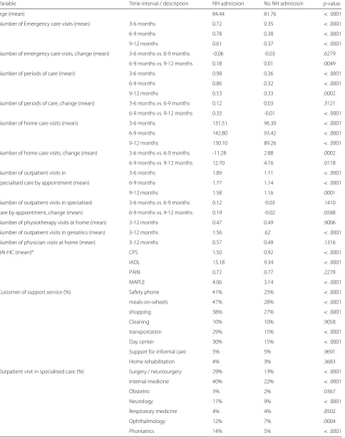
Table 1The characteristics of the study sample (means / %) with and without a nursing home admission and the results of t-tests of significance difference between the means of continuous values or categorical variables
Variable Time interval / description NH admission No NH admission p-value
Age (mean) 84.44 81.76 <.0001
Number of Emergency care visits (mean) 3-6 months 0.72 0.35 <.0001
6-9 months 0.78 0.38 <.0001
9-12 months 0.61 0.37 <.0001
Number of emergency care visits, change (mean) 3-6 months vs. 6-9 months -0.06 -0.03 .6279
6-9 months vs. 9-12 months 0.18 0.01 .0049
Number of periods of care (mean) 3-6 months 0.98 0.36 <.0001
6-9 months 0.86 0.32 <.0001
9-12 months 0.53 0.33 .0002
Number of periods of care, change (mean) 3-6 months vs. 6-9 months 0.12 0.03 .3121
6-9 months vs. 9-12 months 0.33 -0.01 <.0001
Number of home care visits (mean) 3-6 months 131.51 96.30 <.0001
6-9 months 142.80 93.42 <.0001
9-12 months 130.10 89.26 <.0001
Number of home care visits, change (mean) 3-6 months vs. 6-9 months -11.28 2.88 .0002
6-9 months vs. 9-12 months 12.70 4.16 .0118
Number of outpatient visits in 3-6 months 1.89 1.11 <.0001
specialised care by appointment (mean) 6-9 months 1.77 1.14 <.0001
9-12 months 1.58 1.16 .0001
Number of outpatient visits in specialised 3-6 months vs. 6-9 months 0.12 -0.03 .1410
care by appointment, change (mean) 6-9 months vs. 9-12 months 0.19 -0.02 .0588
Number of physiotherapy visits at home (mean) 3-12 months 0.47 0.49 .9006
Number of outpatient visits in geriatrics (mean) 3-12 months 1.56 .62 <.0001
Number of physician visits at home (mean) 3-12 months 0.57 0.49 .1316
RAI-HC (mean)a CPS 1.50 0.92 <.0001
IADL 13.18 9.34 <.0001
PAIN 0.72 0.77 .2278
MAPLE 4.06 3.14 <.0001
Customer of support service (%) Safety phone 41% 25% <.0001
meals-on-wheels 47% 28% <.0001
shopping 38% 27% <.0001
Cleaning 10% 10% .9058
transportation 29% 15% <.0001
Day center 30% 15% <.0001
Support for informal care 5% 5% .9691
Home rehabilitation 4% 3% .3683
Outpatient visit in specialised care (%) Surgery / neurosurgery 29% 13% <.0001
Internal medicine 40% 22% <.0001
Obstetric 3% 2% .0367
Neurology 17% 9% <.0001
Respiratory medicine 4% 4% .8502
Ophthalmology 12% 7% .0004
Table 1The characteristics of the study sample (means / %) with and without a nursing home admission and the results of t-tests of significance difference between the means of continuous values or categorical variables (Continued)
Variable Time interval / description NH admission No NH admission p-value
Psychiatry 14% 9% .0004
Period of care in specialised care (%) Surgery / neurosurgery 20% 8% <.0001
Internal medicine 30% 16% <.0001
Obstetric 0% 0% .5341
Neurology 10% 3% <.0001
Respiratory medicine 2% 2% .5684
Ophthalmology 1% 0% .0028
Phoniatrics 1% 0% .1042
Psychiatry 8% 2% <.0001
Intensive care unit 1% 0% .0211
Diagnosis (%) a00-a09 4% 2% <.0001
a30-a49 4% 3% .1679
e00-e07 3% 2% 0.0723
e10-e14 9% 6% .0037
e70-e90 5% 2% <.0001
f00-f03 50% 16% <.0001
f04-f09 4% 2% .0006
f10-f19 2% 1% .3515
f20-f29 2% 2% .7376
f30-f39 6% 4% .0123
g20-g26 5% 2% .0001
g30-g32 32% 6% <.0001
g40-g47 3% 2% .0972
i10-i15 28% 12% <.0001
i20-i25 14% 6% <.0001
i30-i52 25% 13% <.0001
i60-i69 9% 4% <.0001
i70-i79 3% 1% .0023
i80-i89 2% 1% .1083
i95-i99 5% 1% <.0001
j09-j18 6% 3% .0136
j20-j22 3% 2% .0437
j40-j47 5% 3% .1991
k55-k63 5% 2% <.0001
m05-m14 2% 2% .7376
m15-m19 5% 2% .0005
m45-m49 2% 1% .0008
m50-m54 4% 2% .0933
m70-m79 3% 2% .0978
m80-m85 4% 2% .0008
n10-n16 4% 2% .0324
n17-n19 5% 2% .0001
Table 1The characteristics of the study sample (means / %) with and without a nursing home admission and the results of t-tests of significance difference between the means of continuous values or categorical variables (Continued)
Variable Time interval / description NH admission No NH admission p-value
n40-n51 2% 1% .0813
r00-r09 2% 2% .9037
r10-r19 4% 2% .0034
r40-r46 5% 2% .0012
r50-r69 10% 4% <.0001
s00-s09 8% 2% <.0001
s30-s39 2% 1% .0115
s40-s49 2% 1% .3970
s70-s79 5% 2% <.0001
s80-s89 2% 1% .1098
z00-z13 5% 3% .1123
aResident Assessment Instrument for Home Care (RAI-HC). The Cognitive Performance Scale (CPS) uses items on memory and communication skills to create a 7-point scale
from 0 (intact) to 6 (very seve re) [35]. The Instrumental Activities of Daily Living (IADL) scale [36] provides a measure of the customer’s self-performance of seven daily tasks: meal preparation, ordinary housework, managing finances, managing medications, phone use, shopping and transportation. The scores are from 0 to 21. The Method for Assigning Priority Levels (MAPLe) differentiates customers into five different groups ranging from low to very high risk of health decline [34]. Higher risk group indicates a higher risk to be admitted to a long-term care facility
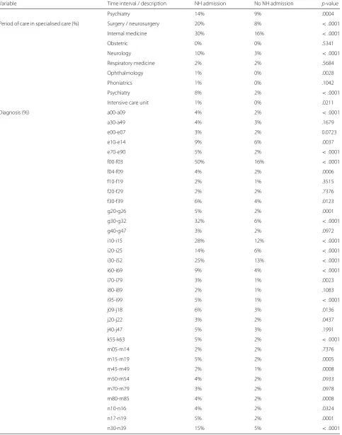
numbers of events or boolean value [true/false] that an event occurred between timestkandtk+1(k=1, 2, 3)or
t1andt4. For example, variablej(a blue box in Fig. 1) for
customeriwas calculated from time periodt2,ij−t3,ij. The interval between timest1andtevwas set to be 12 months andt1< t2 < t3 < t4 < tev. If NHA variable was “true” for the customeri, that is the customeriwas admitted to nursing home at timete,i, timetev,iwas set to be the admis-sion day (→tev,i=te,i). If the NHA variable of customeri
was “false”, then timetev,iwas a random day between times ts,iandte,i, st.tev,i>ts,i+12 months.
Table 1 presents general characteristics of the study sample (n = 3056), of which 539 (17.6%) were admit-ted to nursing home. The table includes the results of t-test of significance difference for continuous variables and chi-squared test for categorical variables between the groups of home caring customers and nursing home residents.
Variable subset selection
The aim of this study was to find efficient variable sub-sets Xsub = {xi|i = 1,. . .n} from a large variable set X = {xj|j = 1,. . .k} for predicting the NHA when n andkare the numbers of variables andn < k. LetY be
the binary vector of NHA variable,F(·)is a classifier and Y = F(Xsub). That is, we predict the state ofYi for cus-tomeriat timetev,i(Fig. 1), when the variable vectorXsub,i is calculated from time ranget1,i−t4,i(3–12 months before tev,i) ort1,i−t3,i(6–12 months beforetev,i).
Variable selection is a mature research topic and has been used for many applications [18]. In this study we applied sequential forward selection (SFS) method [19] for variable subset generation. SFS starts with an empty set and adds one variable at a time from the original setXfor classifier by maximizing the performance measure. Our primary performance metric was classification accuracy:
acc= 1
nsamples nsamples
i=1
Lypred,i=yi
(1)
whereypred,i is the predicted NHA class of thei-th sam-ple, yi is the corresponding true NHA class, nsamples is the number of samples andL(·)is the indicator function (L = 1 if ypred = y; L = 0 if ypred = y) [20]. We additionally calculated the average area under the curve (AUC) and true-positive rate (recall) values for classifiers. AUC values correlated almost perfectly withaccvalues, but we decided to report them, because in some research
Fig. 1Variables were calculated in time periods oft1-t4, whents-teis the time period of home care for a customer. Figure shows time scale of
areas they are more familiar than the accvalues. Recall of a classifier is calculated by dividing the correctly clas-sified positives (true positives) by the total positive count (true positives + false negatives) [21]. That is, recall is the probability that a risk customer is found.
The strength of the accuracy metric, compared to the other common metrics, is that the accuracy metric is easy to understand. It should be noted, that our data set is highly unbalanced. We use a random operator to form bal-anced data sets and the performance results are reported on those balanced data sets instead of the original set. Otherwise, the accuracy metric would be biased and not suitable.
An alternative of SFS would be sequential backward elimination (SBE). SBE starts withXand eliminates one variable at a time by maximizing the performance mea-sure. Our selection of SFS instead of the SBE method is justified by the ratio of relevant (#r) and all (k) variables. According to Liu et al. [18], if #ris small, then the SFS strategy should be used, and if the number of irrelevant variables (k−#r) is small, then the SBE strategy should be used. According to the pre-tests, the original variable set Xincludes many irrelevant variables (low univariate prediction power); thus, we prefer the SFS strategy.
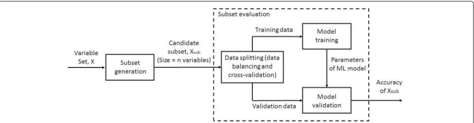
Different classifiers have different performance for dif-ferent data sets. In this study, we evaluated the perfor-mance of three classifiers: logistic regression (LR) [22], Gaussian naive Bayes (GNB) [23] and support vector clas-sifier (SVC) [24]. That is, SFS was run three times using the classifiers of LR, GNB or SVC. Figure 2 shows the components of variable subset selection process. The sub-set generation component (SFS) feeds candidate variable subsetXsub to subset evaluation component. Evaluation component trains and validates classifier and calculates the accuracy values for the subsetXsub.
It should be noted, that we use a random operator to form balanced data sets for the analyses. LetA= {X|Y = 1}andB = {X|Y = 0} be the data sets. That is, the set Acontains the data of customers with the values of “true”
of NHA variable and the Bwith “false”. Because the set A is smaller (n = 539) than the setB(n = 2517), the balanced data setCwas formed, st.C =A∪R(B)where Ris a random operator for selecting 539 random samples fromB, thus setting the level of chance at 50%. To be sure that the selection did not bias the results, data setCwas formed 100 times.
Furthermore, classifier algorithms were trained and val-idated using a ten-fold cross validation method. That is, we formed sampleCi (i = 1,. . ., 100) from the data sets AandB, and split it into 10 equal-sized partsPik (Pik ∈ Ci andk = 1,. . .10). The classification accuracy value, accik, was calculated by Eq. 1 for the partPik of the data setCiwhen the parameters of the classifier were trained with the other K-1 parts of the data set Ci. The process was repeated fork=1, 2,. . .10. The overall classification accuracy,CA, for the subsetXsub,nof size n (n=1,. . .15) was calculated as
CAXsub,n = 1 100∗K
100
i=1 10
K=1
accik (2)
SFS calculated the best variable subsets for all balanced data setsCi. That is, we have 100 variable subsets of size of 1–15 variables. The (average) importance of each variable was measured by a rank metric:
R(j)= 1 100
100
i=1
#F−r(i,j) (3)
wherer(i,j)is the rank of variablejbased on sampleCi and #F is the size of the largest subset that was formed by SFS [25–27]. In this study #F = 15. HigherR(j) indi-cates that variablejis more important according to SFS, because it was selected for smaller size variable subsets. That is, variable has higher prediction capability accord-ing to SFS and its NHA classification ability is high.
Software
We used four Python packages:sklearn[20],mlxtend[28], numpy [29] and pandas [30] to implement the classi-fiers and compute, acc, AUC, recall, CAXsub and R(j). SFS was computed by the function “SequentialFeature-Selector” in the package mlxtend. The classifiers of LR, SVC and GBN were implemented using the func-tions from the sklearn.linear_model, sklearn.svm and sklearn.naive_bayespackages. The packages ofnumpyand pandaswere used for data reading and processing.
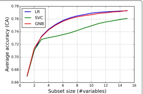
Results
Figure 3 shows the performance (average classification accuracy) of the feature subsets found by different clas-sifiers as a function of the subset size when the variables were calculated 3–12 months before the evaluation day tev. The average classification accuracy values were deter-mined by Eq. 2. The classifiers of LR, SVC and GNB had the average accuracies of 0.776 (CI95% = .0025), 0.762 (CI95%=.0026) and 0.776 (CI95%=.0024), respectively, for the variable subset of 15 variables. According to the student’s t-tests [31], the average classification accuracy value of LR and GNB methods with 15 variables differed statistically from the SVC method: LR vs. SVC (p<.0001) and GNB vs. SVC (p<.0001).
In addition, we calculated average AUC and recall values for the classifiers. The AUC values were 0.846 (CI95%= .0025), 0.838 (CI95%=.0025) and 0.847 (CI95%=.0024) for the classifiers of LR, SVC and GNB with 15 variables. The recall values were 0.755 (CI95% = .0015), 0.724 (CI95% = .0018) and 0.756 (CI95% = .0018). An AUC of 0.5 indicates no discrimination above chance and an AUC of 1.0 indicates perfect classification. A rough guide for the classification ability is AUC 0.9− 1.0 excellent,
Fig. 3Average accuracy as a function of the size of variable subset. Figure shows the classification accuracy of the feature subsets found by different classifiers as a function of the subset size. The average classification accuracy values of LR and GNB methods differ from the SVC method
AUC 0.8−0.9 good, AUC 0.7−0.8 fair and AUC 0.6− 0.7 poor [32]. In general, classification ability is useful if AUC > 0.75 [33]. That is, the performance of the classifiers with 15 variables was at good level.
When the variables were calculated 6–12 months before the evaluation daytev, the average accuracy of classifiers of LR, SVC and GNB were 0.747 (CI95%= .0030), 0.737 (CI95%=.0029) and 0.734 (CI95%=.0029), respectively, for the variable subset of 15 variables. The AUC values were 0.819 (CI95% = .0027), 0.810 (CI95% = .0028) and 0.813 (CI95% = .0025). The recall values were 0.732 (CI95% = .0017), 0.738 (CI95% = .0025) and 0.732 (CI95% = .0026). The results of the 6–12 months vari-ables show a moderate decrease in performance compared to the 3–12 months variables (e.g. LR CA: 0.776→0.747). The performance of the classifiers with the 6–12 months variables, however, is still at good level (AUC>0.8).
Figure 4 shows thep-values calculated by the student’s t-test when the average classification accuracy values for the subsets of 15 variables of 3–12 months were compared to the subsets ofnvariables (n = 1,. . .15). We defined that ifp < .05, the difference between the performances of variable subsets is statistically significant. According to the definition, the optimal subset size for LR method was 9 variables. That is, the performance achieved by the sub-set size of 9 variables did not differ statistically from the subset of 15 variables, when the classifier was LR.
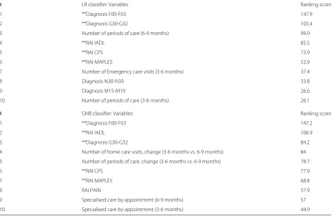
Table 2 sorts the variables according to ranking score,R, described by Eq. 3, for the classifiers of LR and GNB. Large R(j)value means that the variablejwas selected regularly in small variable subsets for different balanced data sets C. That is, the NHA classification ability of the variablej
Table 2The 10 variables of the highest ranking score values calculated for the LR and GNB classifiers (the important variables for the both classifiers are marked as stars)
# LR classifier: Variables Ranking score
1 **Diagnosis F00-F03 147.9
2 **Diagnosis G30-G32 105.4
3 Number of periods of care (6-9 months) 99.9
4 **RAI IADL 85.5
5 **RAI CPS 73.9
6 **RAI MAPLE5 53.9
7 Number of Emergency care visits (3-6 months) 37.4
8 Diagnosis N30-N39 33.8
9 Diagnosis M15-M19 26.6
10 Number of periods of care (3-6 months) 26.1
# GNB classifier: Variables Ranking score
1 **Diagnosis F00-F03 147.2
2 **RAI IADL 106.9
3 **Diagnosis G30-G32 84.2
4 Number of home care visits, change (3-6 months vs. 6-9 months) 84
5 Number of periods of care, change (3-6 months vs. 6-9 months) 78.7
6 **RAI CPS 77.9
7 **RAI MAPLE5 68.8
8 RAI PAIN 57.9
9 Specialised care by appointment (6-9 months) 57
10 Specialised care by appointment (3-6 months) 44.9
is high. According to the results, the most important vari-ables were the diagnoses of G30-G32 and F00-F03 and the RAI metrics of IADL (Activities of Daily Living), MAPLE (Method for Assigning Priority Levels) and CPS (Cogni-tive Performance Scale). In addition, variables related to the numbes of periods of care were important variables for predicting NHA with the both classifiers. It should be noted, that the RAI variables (IADL, MAPLE and CPS) are not simple measurements or observations, but instead scoring systems developed by researcher and practition-ers (e.g., MAPLE [34], CPS [35] and IADL [36]). That is, it is not surprising that these variables have such high performance at predicting NHA.
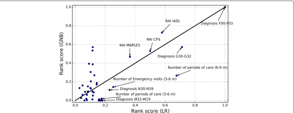
Figures 5 and 6 plot the normalized ranking score val-ues for the classifiers of SVC and GNB as a function of the values of LR. Ten variables with the highest Rvalues of LR classifier are labelled on the figures. The 45◦identity line visualizes the differences between the R values of the classifiers. Variables in the lower-right region of the line were more important for the LR than for the SVC (Fig. 5) or for the GNB (Fig. 6). Similarly, those in the upper-left region were more important for the SVC (Fig. 5) or for the GNB (Fig. 6) than for the LR. For example, the diagnosis N30-N39 was more important for the SVC classifier than
for the LR. However, the differences between the most important variables of the classifier were rather small. The variables of the RAI MAPLE, RAI IADL, RAI CPS and diagnoses F00-F03 and G30-G32 were five important variables for the all classifiers.
Discussion
Fig. 5Normalized ranking score values of the SVC method as a function of the LR method. The variables of the RAI MAPLE, RAI IADL, RAI CPS and diagnoses F00-F03 and G30-G32 were five important variables for the both classifiers
well in advance of the admission. Otherwise, it is too late to implement any interventions. Therefore, the fact that the accuracy of our model with variables 6–12 months before the evaluation day is as high as 74%, is important.
As far as we know, no prior research has published the classification accuracy of the NHA model for individu-als. It should be noted, that the classification accuracy is a very common metric in machine learning and other fields. However, prior research has done the analyses at the pop-ulation level. The important variables have been detected using the 5% level of significance. That is, the values of the parameters of a model (e.g. linear regression (e.g. [12]), logistic regression (e.g. [9, 14]) or Cox model (e.g. [4, 5])) are estimated from whole data (without the split of train and test sets) and the significance levels for coefficients
are derived. Nothing else has done to see if the model gen-eralizes on the data and individuals that played no role in estimating the parameters for models. Few scholars of NHA (e.g. [2, 12]) have applied goodness-of-fit tests (e.g. AIC, R2) for the model, but the test results were often
more close to zero than one (≈.20−.25).
We see that the above lacks in NHA research are related to the public health science and data modelling cultures, in which model validation is omitted or calculated only on training data [37]. In this study we searched the important variables by averaging the results of variable selection that was executed for many random split of the whole data set. The importance of variables was measured by the ranking metric. The level of classification accuracy of model for different variable subsets was tested by cross-validation.
The variable selection from many random data samples and cross-validation warrants the generalization of our variables and models.
The variables of RAI MAPLE, functional impairment (RAI IADL), cognitive impairment (RAI CPS), mem-ory disorders (G30-G32 and F00-F03) and the use of community-based health services and prior hospital use (emergency visits and periods of care) were the most important. The ICD10 (International Classification of Diseases) group of G30-G32 contains the codes for other degenerative diseases of the nervous system (e.g. Alzheimer) and F00-F03 for dementia. A comparison of our results with the findings of the other investigations revealed that especially, functional [1–3, 5–9, 11, 13, 14] and cognitive [2, 5, 8, 9, 11, 14] impairment, dementia [1, 3, 13, 14] and use of community-based health services [2, 4] or prior hospitalization [9] were also strong predictors of NHA. In contrast to our findings, [2, 4–6, 9, 13, 14] found that increased age lead to increased risk of NHA. In our study, the importance of variable of age was rather low according to the ranking score.
The major strengths of this study include its detailed assessment of important variables and model validation and availability of a range of important variables for nurs-ing home admission. The accuracy of the model was high enough to convince the officials of the city of Tampere to integrate the predictive model as a part of home care information system. However, there are some limitations to the present study. We were unable to investigate the associations of social relationships with nursing home admission. Some studies have shown that caregiver char-acteristics [4, 7, 14, 38, 39], having children [8, 9] and marital status [6] can be important factors for NHA. Sec-ond, this was a study of home caring clients living in a defined geographical location, which may limit the gen-eralizability to older adults living in other areas. Also the finding of this study may not be applicable to population without home caring services. In addition, many of the evaluated risk variables found in this study, are not modi-fiable. Further work need to be done to evaluate variables that are modifiable and responsive to interventions.
Practical implications
It is clear, that applying ML methods will progress and reform the work of the gerontology researchers and practitioners. The benefits can be viewed from the two aspects: 1) ML methods can be used to construct prac-tical computer software for predicting NHA to aid the decision-making of practitioners, 2) large variable groups can be studied and the most important variables can be found.
The aspect (1) contributes most to the work of practi-tioners, e.g. home care case managers. The problem the
case managers face is equivalent to that in any preventive care: it is difficult to achieve cost-efficiency if you can-not target a specific subgroup. You usually provide a small intervention for everyone, which is not enough for those at high risk. In order to be effective, the preventive mea-sure needs to be substantial (e.g. in the case of home care customers, 2000e) but becomes too expensive, if offered for many customers. With limited resources one needs to know which customers are most in need of a rehabilita-tion intervenrehabilita-tion and target those individuals to maximize cost-effectiveness.
In the case of home care in Tampere, about 17% of customers are admitted to a nursing home within a year, which is the a priori risk for everyone. The algorithm pro-duced with ML techniques gives a much more accurate risk value enabling the targeting off interventions. With-out an accurate prediction algorithm, it is difficult to iden-tify the high risk individuals. It is not enough to ideniden-tify variables that have a statistically significant relationship with NHA, because this does not provide guidelines that can be applied in practice. For example, we know that a diagnosis indicating dementia or Alzheimer’s disease increases NHA risk, but this information is not specific enough to identify the individuals in need of an inter-vention (unless we target everyone with that particular diagnosis). The ML algorithm provides a risk classifica-tion and also allows for the estimaclassifica-tion of the accuracy of the prediction. Also, in many cases the case managers need to convince their superiors of the need of investing in rehabilitation interventions for a particular customer. The risk estimate from a validated prediction algorithm can be used as a means of communication between the case manager and her superior.
Furthermore, the prediction model can also be used to estimate resource requirements for 24 h services by summing up the individual predictions. The predictions provide an upper limit estimation for capacity require-ment. With time, when data is gathered on by how much targeted rehabilitation interventions can reduce NHA, the capacity estimates become more accurate.
on more objective evaluations and customers are screened regularly. This way it is possible to identify customers at risk earlier than before. Also, after the implementation of the prediction algorithm, the selection of different reha-bilitation interventions available for home care customers has been increased.
The next step in the study and implementation project is to gather data from the interventions and their effects, and build another ML model to predict the effectiveness of each intervention for each type of customer. Also, the model can be used to predict, who is no longer capable of benefitting from an intervention. This added information will further improve the cost-effectiveness of home care.
The aspect (2) contributes both the gerontology research and practical work. Variable selection can be used to identify which of the available variables are closely related to the prediction of the NHA and to discard those unrelated to it, reducing the dimensionality of the dataset. For the researcher of gerontology, the process of variable selection may indicate new variables that had not been previously considered as relevant to NHA. For example, in this study, we found about 10 important variables for predicting NHA. Furthermore, the model validity is eas-ier to evaluate after variable selection is used to reduce the dimensionality of the model. After dimension reduction, the researchers know the variables for which they should focus in their research [40]. For the NHA research, this may mean that the variables for which the interventions should be focused can be found.
The second benefit, because of the variable selection, is that the number of variables, integrated in the software tool, can be minimized. This is important, because each new added variable requires resources for the processes of data aggregation and validation and requirements for data integration from different databases.
Conclusion
Most elderly people prefer to live at home in a familiar environment than move to a nursing home. The find-ings of our study indicate important variable subsets for predicting NHA of community dwelling home care cus-tomers, and offer potential to find those individuals at the level of 78%, who are at risk of NHA. The most important variables were RAI MAPLE, functional impairment (RAI IADL), cognitive impairment (RAI CPS), memory disor-ders (diagnoses G30-G32 and F00-F03) and the use of community-based health-service and prior hospital use.
Endnotes
1Tampere is the third largest city in Finland. The
per-cent of population over 65 years is 18.0% that is approx-imately same as in the other big cities in Finland (http:// www.stat.fi). Also, the scope or services offered for the
elderly as well as eligibility criteria for home care and nursing home care are fairly similar in all areas in Finland.
2Kotitori http://www.tampereenkotitori.fi/
Abbreviations
AUC: Area under the curve; CA: Classification accuracy; CPS: Cognitive performance scale; GNB: Gaussian naive Bayes; IADL: Activities of daily living; LR: Logistic regression; MAPLE: Method for assigning priority levels; ML: Machine learning; NHS: Nursing home admission; RAI-HC: Resident assessment instrument - home care; SBE: Sequential backward elimination; SFS: Sequential forward selection; SVM: Support vector machine
Acknowledgements
The authors would like to thanks Mr. Mikko Mulari for his contribution for data acquisition and interpretation.
Funding
The study was independent of external funding sources.
Availability of data and materials
The dataset which we have acquired will not be shared as a supplementary file. All Python codes for data analysis and variable subset selection are available upon request.
Authors’ contributions
MN participated in the data collection, study design, performed the literature review, programming all analyses and wrote the first draft of the paper. RLL contributed to the design of the study, interpretation of the results and was involved in writing of the first draft of the paper. ES and AT participated to the design of the study and revised the paper. VK managed and supervised the study, participated to the design of the study and revised the paper. All authors read and approved the final manuscript.
Competing interests
MN: employment (Nordic Healthcare Group), RLL and VK: employment and stockholder (Nordic Healthcare Group). Nordic Healthcare Group (NHG) is a Finnish company specialised in planning and developing health and social services especially in Finland, Sweden and Russia. ES and AT declare that they have no competing interests.
Consent for publication
Not applicable.
Ethics approval and consent to participate
The data were provided by the city of Tampere and Pirkanmaa Hospital District who granted us the research promises and the privilege to use the data. Data were aggregated and anonymized by the data administration of the city of Tampere before they were provided to the authors. Ethics approval was not required. In Finland, ethics approval is not required for retrospective registry studies with anonymized data. Since this was a retrospective study, consent to participate was not required.
Publisher’s Note
Springer Nature remains neutral with regard to jurisdictional claims in published maps and institutional affiliations.
Author details
1Nordic Healthcare Group, Vattuniemenranta 2, 00210 Helsinki, Finland.2City
of Tampere, PL 487, 33101 Tampere, Finland.
Received: 23 November 2016 Accepted: 7 April 2017
References
1. Hajek A, Brettschneider C, Lange C, Posselt T, Wiese B, Steinmann S,
2. Sørbye L, Hamran T, Henriksen N, Norberg A. Home care patients in four nordic capitals — predictors of nursing home admission during one-year followup. J Multidiscip Healthc. 2010;3:11–18. doi:10.2147/JMDH.S8979.
3. Gnjidic D, Stanaway F, Cumming R, Waite L, Blyth F, Naganathan V,
Handelsman DJ, Le Couteur DG. Mild cognitive impairment predicts institutionalization among older men: A population-based cohort study. PLoS ONE. 2012;7(9):1–8. doi:10.1371/journal.pone.0046061.
4. Eska K, Graessel E, Donath C, Schwarzkopf L, Lauterberg J, Holle R.
Predictors of institutionalization of dementia patients in mild and moderate stages: A 4-year prospective analysis. Dement Geriatr Cogn Disord Extra. 2013;3(1):426–45. doi:10.1159/000355079.
5. Luppa M, Luck T, Matschinger H, König HH, Riedel-Heller SG. Predictors
of nursing home admission of individuals without a dementia diagnosis before admission - results from the leipzig longitudinal study of the aged (leila 75+). BMC Health Serv Res. 2010;10(1):1–8.
doi:10.1186/1472-6963-10-186.
6. Andel R, Hyer K, Slack A. Risk factors for nursing home placement in
older adults with and without dementia. J Aging Health. 2007;19(2): 213–8. doi:10.1177/0898264307299359.
7. Jiska C, Philip W. Predictors of entry to the nursing home: Does length of
follow-up matter? Arch Gerontol Geriatr. 2011;53(3):309–15. doi:10.1016/j.archger.2010.12.009.
8. Dramé M, Lang P, Jolly D, Narbey D, Mahmoudi R, Lanièce I, Somme D,
Gauvain J, Heitz D, Voisin T, de Wazières B, Gonthier R, Ankri J, Saint-Jean O, Jeandel C, Couturier P, Blanchard F, Novella J. Nursing home admission in elderly subjects with dementia: predictive factors and future challenges. J Am Med Dir Assoc. 2013;13:17–20.
doi:10.1016/j.jamda.2011.03.002.
9. Akamigbo A, Wolinsky F. Reported expectations for nursing home
placement among older adults and their role as risk factors for nursing home admissions. Gerontologist. 2006;46:464–73.
doi:10.1093/geront/46.4.464.
10. Sheppard K, Brown C, Hearld K, Roth D, Sawyer P, Locher J, Allman R, Ritchie CS. Symptom burden predicts nursing home admissions among older adults. J Pain Symptom Manage. 2013;46:591–7.
doi:10.1016/j.jpainsymman.2012.10.228.
11. von Bonsdorff M, Rantanen T, Laukkanen P, Suutama T, Heikkinen E. Mobility limitations and cognitive deficits as predictors of
institutionalization among community-dwelling older people. Gerontology. 2006;52(6):359–65. doi:10.1159/000094985.
12. Chen C, Naidoo N, Er B, Cheong A, Fong NP, Tay CY, Chan KM, Tan BY, Menon E, Ee CH, Lee KK, Ng YS, Teo YY, Koh GCH. Factors associated with nursing home placement of all patients admitted for inpatient rehabilitation in singapore community hospitals from 1996 to 2005: A disease stratified analysis. PLoS ONE. 2013;8(12):1–11.
doi:10.1371/journal.pone.0082697.
13. Wergeland J, Selbæk G, Bergh S, Soederhamn U, Kirkevold . Predictors for nursing home admission and death among community-dwelling people 70 years and older who receive domiciliary care. Dement Geriatr Cogn Disord Extra. 2015;5:320–9. doi:10.1159/000437382.
14. Sheppard K, Sawyer P, Ritchie C, Allman R, Brown C. Life-space mobility predicts nursing home admission over 6 years. J Aging Health. 2013;25: 907–20. doi:10.1186/1471-2318-7-13.
15. Helvik AS, Skancke RH, Selbæk G, Engedal K. Nursing home admission during the first year after hospitalization? the contribution of cognitive impairment. PLoS ONE. 2014;9(1):1–7. doi:10.1371/journal.pone.0086116. 16. Gaugler J, Duval S, Anderson K, Kane R. Predicting nursing home
admission in the u.s: a meta-analysis. BMC Geriatr. 2007;13:1–14. doi:10.1186/1471-2318-7-13.
17. Morris J, Fries B, Bernabei R, Steel K, Ikegami N, Carpenter I, Gilgen R, DuPasquier J, Frijters D, Henrard J, Hirdes J, Belleville-Taylor P, Berg K, Björkgren M, Gray I, Hawes C, Ljunggren G, Nonemaker S, Phillips C, Zimmerman D. interRAI Home Care (HC) Assessment Form and User’s Manual. USA: interRAI; 2009.
18. Liu H, Yu L. Toward integrating feature selection algorithms for classification and clustering. IEEE Trans Knowl Data Eng. 2005;17(4): 491–502. doi:10.1109/TKDE.2005.66.
19. Hastie T, Tibshirani R, Friedman J. The Elements of Statistical Learning. New York: Springer; 2009.
20. Pedregosa F, Varoquaux G, Gramfort A, Michel V, Thirion B, Grisel O, Blondel M, Prettenhofer P, Weiss R, Dubourg V, Vanderplas J, Passos A,
Cournapeau D, Brucher M, Perrot M, Duchesnay E. Scikit-learn: Machine Learning in Python. J Mach Learn Res. 2011;12:2825–830.
21. Olson DL, Delen D. Advanced Data Mining Techniques. Germany: Springer-Verlag Berlin Heidelberg; 2008. doi:10.1007/978-3-540-76917-0. 22. McCullagh P, Nelder JA. Generalized Linear Models, (Second Edition).
London: London: Chapman & Hall; 1989, p. 500.
23. Zhang H. The optimality of naive bayes In: Barr V, Markov Z, editors. Proceedings of the Seventeenth International Florida Artificial Intelligence Research Society Conference (FLAIRS 2004). Palo Alto: AAAI Press; 2004. 24. Cortes C, Vapnik V. Support-vector networks. Mach Learn. 1995;20(3):
273–97. doi:10.1023/A:1022627411411.
25. Xin L, Zhu M. Stochastic stepwise ensembles for variable selection. J Comput Graph Stat. 2012;21(2):275–94.
doi:10.1080/10618600.2012.679223.
26. Cheng L, Zhu M, Poss JW, Hirdes JP, Glenny C, Stolee P. Opinion versus practice regarding the use of rehabilitation services in home care: an investigation using machine learning algorithms. BMC Med Inform Decis Mak. 2015;15(1):1–11. doi:10.1186/s12911-015-0203-1.
27. Liu N, Koh ZX, Goh J, Lin Z, Haaland B, Ting BP, Ong MEH. Prediction of adverse cardiac events in emergency department patients with chest pain using machine learning for variable selection. BMC Med Inform Decis Mak. 2014;14(1):75. doi:10.1186/1472-6947-14-75.
28. Raschka S. Mlxtend. 2016. doi:10.5281/zenodo.49235. http://dx.doi.org/ 10.5281/zenodo.49235. Accessed 8 Feb 2016.
29. Jones E, Oliphant T, Peterson P, et al. SciPy: Open source scientific tools for Python. 2001. http://www.scipy.org/. Accessed 15 Aug 2016. 30. McKinney W. Data structures for statistical computing in python. In:
Proceedings of the 9th Python in Science Conference, SciPy.org. van der Walt, S., Millman, J. (eds.). 2010. p. 51–56. http://conference.scipy. org/proceedings/.
31. Wilcox R. Basic Statistics: Understanding Conventional Methods and Modern Insights. New York: Oxford University Press; 2009. 32. Roelen CA, Bültmann U, van Rhenen W, van der Klink JJ, Twisk JW,
Heymans MW. External validation of two prediction models identifying employees at risk of high sickness absence: cohort study with 1-year follow-up. BMC Public Health. 2013;13(1):1–8.
doi:10.1186/1471-2458-13-105.
33. Fan J, Upadhye S, Worster A. Understanding receiver operating characteristic (roc) curves. Can J Emerg Med. 2006;8(1):19–20. doi:10.1017/S1481803500013336.
34. Hirdes J, Poss J, Curtin-Telegdi N. The method for assigning priority levels (maple): A new decision-support system for allocating home care resources. BMC Med. 2008;6(1):1–11. doi:10.1186/1741-7015-6-9. 35. Morris J, Fries B, Mehr D, Hawes C, Philips C, Mor V, Lipsitz L. Mds
cognitive performance scale. J Gerontol Med Sci. 1994;49(4):174–82. doi:10.1093/geronj/49.4.M174.
36. Spector W, Fleishman J. Combining activities of daily living with instrumental activities of daily living to measure functional disability. J Gerontol B Psychol Sci Soc Sci. 1998;53(1):46–57.
doi:10.1093/geronb/53B.1.S46.
37. Breiman L. Statistical modeling: The two cultures (with comments and a rejoinder by the author). Statist Sci. 2001;16(3):199–231.
doi:10.1214/ss/1009213726.
38. Gaugler J, Yu F, Krichbaum K, Wyman J. Predictors of nursing home admission for persons with dementia. Med Care. 2009;47(2):191–8. doi:10.1097/MLR.0b013e31818457ce.
39. Donnelly NA, Hickey A, Burns A, Murphy P, Doyle F. Systematic review and meta-analysis of the impact of carer stress on subsequent institutionalisation of community-dwelling older people. PLoS ONE. 2015;10(6):1–19. doi:10.1371/journal.pone.0128213.