ISSN (Online): 2320-9364, ISSN (Print): 2320-9356
www.ijres.org Volume 3 Issue 6 ǁ June 2015 ǁ PP.43-47
Solving the Kinematics of Welding Robot Based on ADAMS
Fenglei Sun
1, Yong Xu
21(College of Mechanical Engineering, Shanghai University of Engineering Science, China) 2(College of Mechanical Engineering, Shanghai University of Engineering Science, China)
Abstract
: To solve the problem of angle coupling of the welding robot kinematics equations, we build the 3D model of the welding robot plus kinematics equations via using method of D-H, and taking PUMA560 robot as the study target and using ADAMS software as the simulating tool, through this we achieve the displacementcurve along x, y and z axis. Because of the similar of the result of simulating and one of the positive kinematics equations, this paper verifies the correctness of its 3D model. Based on this, this paper uses the analytic method to deduce the welding robot inverse kinematics equation. This paper only use the derivation method to solve the
problem of the coupling between angles and deduce the formulas of each angle. And this method could be the basis of the welding robot trajectory planning.
Keywords
: welding robot; kinematics; analytic solution; ADAMSI.
Introduction
Researching the inverse kinematics of the welding robot is a very important topic in the kinematics and the trajectory planning. It is very difficult to build the general algorithm because the inverse kinematics of robot is becoming more and more difficult along the increasing of the robot sports joints. In resent years, to solve the inverse kinematics equation, we put forward the analytic method, forward analytic method[1], iterative method[2], geometric method[3], neural network theory and so on. Under these methods, Paul[4] and Wang Qizhi put forward the analytic method, but the problem is that some reverse answers they put forward are not the correct answers. Besides this, Liu song guo, Wang hongbin, and Chen Ning put forward the methods of iterative method and new analytic method, but these cannot correctly calculate the angle via extracting enough elements. So, to solve the angle coupling problem, and to conveniently solve the sine and cosine of each angle, this paper analysis the inverse kinematics answer aimed at the PUMA560 welding robot, using the single or serial matrix 1
1) (Aii
left multiply the matrix 6 0
A , so the right of the equation would not include this angle, so that we could find the
elements that produce the value of the sine and cosine. Under this, we could achieve the correct angle and finish the problem of solving the inverse kinematics equation.
II.
The Positive Kinematics Model of Robot
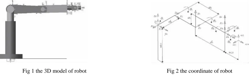
[5]The analysis of kinematics of welding robot is the basis of the research of the trajectory planning, including the problem of positive kinematics and inverse kinematics. And the model of the positive kinematics is the key of building inverse kinematics. So, this paper firstly build the positive model of the welding robot, using PUMA560 robot as the research object. Secondly, this paper use ADAMS[6] software do the simulation. Lastly, comparing the two results, we validated the positive kinematics that built is correct, and which is a basis of the analytic of inverse kinematics of the welding robot.
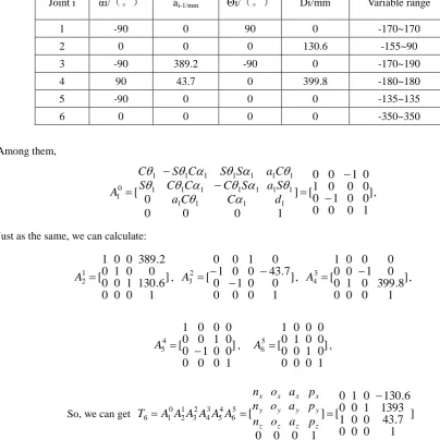
This paper show the relatives of the connection of the two rod coordinate systems via using the method of D-H. And the space relationship of the two adjacent links is a connection link transformation matrix. Building the homogeneous transformation matrix as follow:
]
1
0
0
0
0
[
1 1 1 1 1 1 1 1 1 1 1 1 1 1 1 1 1 1
i i i i i i i i i i i i i i i i i i id
C
S
S
a
S
C
C
C
S
C
a
C
S
C
S
C
A
Among the matrix, C=cos, S=sin, αi-1 is the distance between zi-1 and zi measuring along xi-1; as the same, ai-1 is the rotation angle; di is the distance along zi; θi is the rotation angle around zi; xi, yi, zi are the coordinate system of joint i. According to the matrix above, we achieve the following positive kinematics equation:
] 1 0 0 0 ) ( ) ( ) ( ) ( ) ( ) ( [ ] 1 0 0 0 [ 2 2 3 23 4 234 5 234 6 234 6 5 234 6 234 6 5 234 2 2 3 23 4 234 1 5 1 5 234 1 6 5 1 6 234 6 5 234 1 6 5 1 6 234 6 5 234 1 5 2 3 23 5 234 1 5 1 5 234 1 6 5 1 6 234 6 5 234 1 6 5 1 6 234 6 5 234 1 5 6 4 5 3 4 2 3 1 2 0 1 6 a S a S a S S S C C C C S C C C C S a C a C a C S C C S C S S S C S S C C C S C C C S S C C C S a C a C a C C C S S C C S S S C S C C C C S S S S S C C C C p a o n p a o n p a o n A A A A A A T z z z z y y y y x x x x (1) In this equation, 5
6 4 5 3 4 2 3 1 2 0
1,A ,A ,A ,A ,A
A are the coordinate systems, shoulder coordinate relative to base relative, the big arm coordinate relative to shoulder coordinate, the small arm coordinate relative to the big coordinate, and wrist 1 coordinate relative to the small arm, wrist 2 relative to wrist 1, and wrist 3 coordinate relative to wrist 2 coordinate. Besides,
] [ z z z y y y x x x a o n a o n a o n
is the attitude matrix, ] [ z y x p p p
is the location matrix; C234
represent
cos(
2
3
4)
; S234 representsin(
2
3
4)
.2.2 The Calculation of Positive Kinematics of Welding Robot
Table 1 the parameters of the robot joints
Joint i αi/(。) ai-1/mm Θi/(。) Di/mm Variable range
1 -90 0 90 0 -170~170
2 0 0 0 130.6 -155~90
3 -90 389.2 -90 0 -170~190
4 90 43.7 0 399.8 -180~180
5 -90 0 0 0 -135~135
6 0 0 0 0 -350~350
Among them,
]
1
0
0
0
0
0
1
0
0
0
0
1
0
1
0
0
[
]
1
0
0
0
0
[
1 1 1 1 1 1 1 1 1 1 1 1 1 1 1 1 1 1 0 1
d
C
C
a
S
a
S
C
C
C
S
C
a
S
S
C
S
C
A
,Just as the same, we can calculate:
]
1
0
0
0
6
.
130
1
0
0
0
0
1
0
2
.
389
0
0
1
[
1 2
A
,]
1
0
0
0
0
0
1
0
7
.
43
0
0
1
0
1
0
0
[
2 3
A
,]
1
0
0
0
8
.
399
0
1
0
0
1
0
0
0
0
0
1
[
3 4
A
,]
1
0
0
0
0
0
1
0
0
1
0
0
0
0
0
1
[
45
A
,]
1
0
0
0
0
1
0
0
0
0
1
0
0
0
0
1
[
5 6
A
,So, we can get
]
1
0
0
0
7
.
43
0
0
1
1393
1
0
0
6
.
130
0
1
0
[
]
1
0
0
0
[
5 6 4 5 3 4 2 3 1 2 0 1 6
z z z z y y y y x x x xp
a
o
n
p
a
o
n
p
a
o
n
A
A
A
A
A
A
T
Further, we can get the posture of the end of the robot, as the following, it is the same as the posture that we got in the ADAMS software:
]
1
0
0
0
8
.
665
0
0
1
904
1
0
0
6
.
130
0
1
0
[
]
1
0
0
0
3
.
73
1
0
0
0
0
1
0
0
0
0
1
][
1
0
0
0
7
.
43
0
0
1
1393
1
0
0
6
.
130
0
1
0
][
0
0
0
0
2
.
578
1
0
0
0
0
1
0
0
0
0
1
[
6 0
T
According the simulation in ADAMS, we could got the displacement curve of the end of the welding robot. The curves could be seen in fig 3.
(3) displacement curve along z Fig 3 displacement curve of the end of robot
III.
The Analysis of Inverse Kinematics of Robot
The algorithm of inverse kinematics is the basis of trajectory planning of the robot. But there are a lot of coupling angles when we facing the equations of the kinematics. To solve this problem, to achieve the value of cosine and sine of each angle, this paper use one or serial matrix 1
1)
(Aii multiply matrix 6 0
A on the left so that this equation would not include this angle. Via this method, we can find the elements that produce the values of cosine and sine. Then, we can achieve the angle that we want, finishing the analysis of inverse kinematics of the robot.
3.1 the equation of inverse kinematics solving
According to the positive kinematics equation (1), we could achieve the following valve of
1~
6, details as follow:(1)
1 solving:Using
(
A
10)
1 multiply left both side of equation (1), we can get:]
1
0
0
0
0
)
)
)
[
]
1
0
0
0
][
1
0
0
0
0
0
0
1
0
0
0
0
[
5 6
5 6
5
2 2 3 23 4 234 5 234 6 234 6 5 234 6
234 6 5 234
2 2 3 23 5 234 5 234 6 234 6 5 234 6
234 6 5 234
1 1
1 1
C
S
S
C
C
a
S
a
S
a
S
S
S
C
C
C
C
S
S
S
C
C
C
a
C
a
C
a
C
S
C
C
S
C
C
C
S
S
C
C
C
p
a
o
n
p
a
o
n
p
a
o
n
C
S
S
C
z z z z
y y y y
x x x x
According to the above equation, the value of the third and the fourth line should equal, we achieve
that, 0, , ( ), , 180
1 1 1
1
1 or
p p arcran Then
C p S p
y x y
x
Just as the same methods we solve the value of
1, we can also get the value of
2~
5. Seeing as the following:)
arctan(
3 3 3
C
S
,
2
234
3
4,y x
z y
x
a
C
a
S
a
S
a
S
a
C
C
1 1
234 1
1 234 5
)
(
arctan
,z y
x
z y
x
o
C
o
S
o
C
S
n
C
n
S
n
C
S
234 1
1 234
234 1
1 234 6
)
(
)
(
arctan
Obviously, they are the same with the value in table 1. So this paper correctly validate the equations of inverse kinematics.
IV.
Conclusion
This paper use the analytic method deduce the equations of inverse kinematics so that we can solve the problem of the coupling between angles. Via the solving process, this paper deduced each value of
6 1~
.
And according to the equations of them, it may has 8 inverse answers. But because of the limit of the robot structure, each joint could not achieve the rotation of 360 degrees. So we just need to choose a best answer to meet the working requirements of the robot based on the limits. This algorithm apply to the situation that the last three joints has a public intersection, or it can only be solved through solving the matrix or calculating the inverse of the matrix. As we all know, most industrial robots have the wrist joints.
REFERENCES
[1] Zhiqi Wang, Xinhe Xu, Chaowang Yi. PUMA new derivation and solution for inverse kinematic equation of manipulator. Robot,
02,1998, 81-87
[2] Songguo Liu, Shiqiang Zhu, Jiangbo Li. SResearch on real time inverse kinematics algorithm for robot. Control theory and
application, 25, 2008, 1037-1041.
[3] Yuchao Liu, Yumei Huang, Xiaoyue Huang,. Inverse kinematics of robot kinematics based on genetic algorithm.
Robot.20,1998,421-426
[4] Paul RP, Shimano BE, Mayer G. Kinematic Control Equations for Simple Manipulators. IEEETRANS SMC, 1981,11,449-455
[5] Zixing Cai,. Robotics. Qinghua university press, 2000.