Sentiment Classification: A Topic Sequence-Based
Approach
Xuliang Song
1*, Jiguang Liang
2, Chengcheng Hu
21 National Engineering Laboratory for Information Security Technologies, Institute of Information
Engineering, Chinese Academy of Sciences, Beijing, China.
2 Institute of Information Engineering, Chinese Academy of Sciences, Beijing, China.
* Corresponding author. Tel.: +86-10-82546715; email: [email protected] Manuscript submitted February 9, 2015; accepted May 5, 2015.
doi: 10.17706/jcp.11.1.1-9
Abstract: With the development of Web 2.0, sentiment analysis has been widely used in many domains, such as information retrieval (IR), artificial intelligence and social networks. This paper focuses on the task of classifying a textual review as expressing a positive or negative sentiment, a core task of sentiment analysis called sentiment classification. To address this problem, we present a novel sentiment classification model based on topic sequence which refers to topics in descending order of their distribution probabilities. Topics’ distribution probabilities are obtained after training the latent dirichlet allocation (LDA) model. To the best of our knowledge, previous work didn’t consider the importance of the order relationships among topics. We work on exploiting the order relationships among topics and using this information for sentiment classification. Based on it, three steps are followed to tackle this task. First, we train the LDA model to get the topic distribution. Then, we sort these topics in descending order to get the topic sequence, which are used to construct topic co-occurrence matrices (positive and negative). Finally we use these two matrices to classify the test examples as positive or negative. The experiments show that our classification model obtains better results than many existing classifiers and the topic sequence plays an important role for sentiment classification.
Key words: Latent dirichlet allocation, sentiment analysis, sentiment classification, topic sequence.
1.
Introduction
Therefore, sentiment analysis not only has important social significance, but also becomes a popular topic in many research fields, such as information retrieval (IR) [3], artificial intelligence [4], [5] and social networks [6], [7].
Previous works use topic distributions as features to classify sentiments. They assume that similar documents have similar topic distributions. Unlike to them, we try to exploit the order relationships among topics for sentiment classification. We propose a novel sentiment classifier model called topic co-occurrence matrix (TCOM) and conduct experiments to show that TCOM is an effective model for sentiment classification.
The rest of the paper is organized as follows. In the next Section, we introduce the related work. The classification algorithm is described in Section 3. In Section 4, we describe the experimental results to show the effectiveness of our model. Finally, Section 5 concludes our work and discusses future work.
2.
Related Work
Sentiment classification is a complicated problem but significant research effort has been done, especially in the field of product reviews, movie reviews and microblogs. Pang et al. [2] tried to use machine leaning model to solve this problem. They used n-gram model and compared the effect of three classifiers: Naïve Bayes (NB), Maximum Entroy (ME) and Support Vector Machine (SVM), the experimental results found that with unigram, SVM will obtain the best classification accuracy. Go et al. [8] introduced a novel approach using distant supervision for automatically classifying the sentiment of Twitter messages. Jiang et al. [9] addressed target-dependent Twitter sentiment classification. Given a query, they classified the sentiments of tweets as positive, negative or neutral. Riloff et al. [10] constructed emotional templates for sentiment classification. [11] used words as features to classify the sentiments based on Naïve Bayes classifier. Glorot et al. [12] proposed a deep learning approach to tackle this task by extracting a meaningful representation for each review in an unsupervised fashion.
Because of the high feature dimension of traditional feature representation methods, they usually contain a lot of useless features and can’t capture the main meanings of the document. Therefore, it is necessary to remove the useless features in order to increase the accuracy of classification results. As a feature extraction method, it is worth mentioning that LDA has been successfully used to sentiment classification in recent years. LDA is one of the most popular topic models, it assumes that documents are mixture of topics where a topic is a probability distribution over words. LDA can reduce the number of features significantly. Lin and He [13] proposed a novel probabilistic modelling framework based on LDA, called joint sentiment/topic model (JST), which was fully unsupervised. Li et al. [14] presented a sentiment-LDA model for sentiment classification with global topics and local dependency. Jo and Oh [15] proposed two models, Sentence-LDA (SLDA) and Aspect and Sentiment Unification Model (ASUM) to tackle the problem of automatically discovering what aspects are evaluated in reviews and how sentiments for different aspects are expressed. Although LDA has been applied to sentiment classification for many years, there is little effort done to explore the order relationships among topics.
3.
Method
As proposed in Section 1, we focus on the task of sentiment classification. In this Section, we will present a new classification model based on topic sequence for sentiment classification: Topic Co-occurrence Matrix (TCOM).
3.1.
Latent Dirichlet Allocation
[16]n-gram language model to tackle this problem, however, the number of dimension will be enormous and the computation will be intensive which is known as curse of dimensionality. There are many methods to reduce the feature dimension such as Information Gain, Chi-square test, LDA and so on. LDA is a generative model for collections of discrete data such as text corpora. It is a three-level hierarchical Bayesian model, in which each item of a collection is modeled as a finite mixture over an underlying set of topics, each topic is, in turn, modeled as an infinite mixture over an underlying set of topic probabilities. The graphical model representation of LDA is shown in Fig. 1 and the meanings of the notations are explained in Table 1.
Table 1. Meanings of the Notations
Notation Meaning
M number of documents
N number of words in a document
K number of topics
w words in a document
z topics in a document
θ multinomial distribution over topics
φ multinomial distribution over words
α Dirichlet prior vector for θ
β Dirichlet prior vector for φ
N
M
K α
θ
z
w φ β
Fig. 1. Graphical model representation of LDA.
As can be seen from Fig. 1, LDA contains three layers: document layer, topic layer and word layer, the generative process for each document w in a corpus D is assumed as follows:
1) Choose N ~Poisson(). 2) Choose ~Dir().
3) For each of the N words wn:
a) Choose a topic zn~ Multinomial()
b) Choose a word wn fromp(wn | zn,), a multinomial probability conditioned on the topic zn
A k-dimensional Dirichlet random variable can take values in the (k-1)-simplex (a k-vectorlies in the (k-1)-simplex if i 0,
ik1i 1), and has the following probability density on this simplex:1 ... 1 1 1
1 1
) (
) (
) |
(
k
k k
i i
k
i i
p
(1)
generating a corpus. Given the parametersand, the joint distribution of a topic mixture , a set of N topics z, and a set of N words w is given by:
N
n n n n
z w p z p p w z p 1 ) , | ( ) | ( ) | ( ) , | , ,
( (2)
where p(zn |) is simply i for the unique i such that 1
i n
z . Integrating overand summing overz, we obtain the marginal distribution of a document:
p p z pw z d
w
p N
n zn n n n
)
(
1 ) , | ( ) | ( ) | ( ) , |( (3)
Finally, taking the product of the marginal probabilities of single documents, we obtain the probability of a corpus:
M d d Nn z dn d dn dn
d pz pw z d
p D p d dn 1 1
)
(
( | )( | , ) ) | ( ) , |( (4)
The variables dare document-level variables, sampled once per document. The variables zdn and
dn
w are word-level variables and are sampled once for each word in each document.
3.2.
Topic Sequence and Topic Co-occurrence Matrix
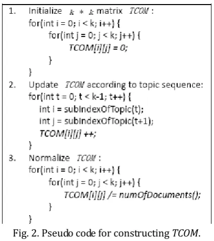
As what we present in Section 1, we explore the order relationships among topics for sentiment classification. We can get the topic distribution after training the LDA model. Instead of putting the topics’ probability into the classifier directly, we sort these topics in descending order to get the topic sequence. Topic sequence means a set of topics in descending order according to their probability. Two adjacent topics in the topic sequence are considered as co-occurrence topics. Then, topic co-occurrence matrix is constructed according to the topic sequence. The pseudo code for constructing the topic co-occurrence matrix is shown in Fig. 2.
Fig. 2. Pseudo code for constructing TCOM.
follows:
1) Initialize the TCOMk k* with value 0, we can get the TCOM as Fig. 3.
0 0 0 0 0 0 0 0 0
Fig. 3. Initialize the TCOM.
2) We consider two adjacent topics as co-occurrence topics in the topic sequence. For each training document, we can get a topic sequence. The TCOM is updated by scanning all of the topic sequences. Take a topic sentence “t2, t1, t0” as an example, when scanning t2 and t1, we update TCOM[2][1] to TCOM[2][1] 1 , then t1 and t0 are scanned, we updateTCOM[1][0]toTCOM[1][0] 1. Assume that we get another topic sequence “t2, t0, t1”, the progress of updating theTCOM is shown in Fig. 4.
0 0 0 0 0 0 0 0 0
t2 t1 t0
0 1 0 0 0 1 0 0 0
Update t2 t0 t1
0 1 1 0 0 1 0 1 0 Update
Fig. 4. The progress of updating the TCOM.
3) After step 2, TCOM will be normalized by dividing the number of documents to get the final TCOM just as Fig. 5 shows.
0 1 1 0 0 1 0 1 0 0 5 . 0 5 . 0 0 0 5 . 0 0 5 . 0 0 Normalization
Fig. 5. The normalization of the TCOM.
3.3.
Classification Algorithm Based on
TCOM
In Section 3.2, we illustrate the process of how to get the TCOM. In this Section, in order to take advantage of the topics’ order relationships, we design a novel classification algorithm based on TCOM. The steps of the classification algorithm are as follows:
1) For positive training data, we get its TCOMPOS using the method which Section 3.2 describes.
2) We get the negative TCOMNEG according to the negative training data.
3) In the classification step, given a test case, we get its TCOMTEST . Then we compute the distance between
TEST
TCOM and TCOMPOS, named as DISPOS, and the distance between TCOMTEST and TCOMNEG, named as
NEG
DIS . The formula to calculate the distance DIS between two matrixes T1 and T2 is shown as
follows.
1 0 1 0 2 2 1)
(
[ ][ ] [ ][ ] k i k j j i T j i TDIS (5)
Finally, we obtain the test case’s classification result by comparing the DISPOS and DISNEG , if
NEG
POS DIS
4.
Experiments
In this Section, we report our datasets, performance measurement, baseline and experimental results. All of the experiments are performed based on 10-fold cross validation.
4.1.
Data Set
We use Chinese sentiment corpora ChnSentiCorp [17] as our corpus. More specifically, we use ChnSentiCorp-Htl-ba-4000 and ChnSentiCorp-NB-ba-4000 corresponding to the domains hotel and computer to test our method. The statistical information of the corpora we used is shown in Table 2.
Table 2. Statistics of ChnSentiCorp
Domain Total
Number
Positive Number
Negative Number
Hotel 4000 2000 2000
Computer 4000 2000 2000
As Table 2 shows, the total number of both corpora is 4000. And the positive number is the same as negative number in both corpora, meaning that the corpora are balanced.
4.2.
Performance Measurement
We evaluate the classification performance in terms of three commonly used metrics: precision, recall and F-measure (
F
1 score) as defined referring to (6)-(8). The confusion matrix is shown in Table 3 whoseentries are given as a function of two classes in document-level sentiment classification, positive and negative documents. Each column of the matrix represents the instances in a predicted class, while each row represents the instances in an actual class.
Table 3. Confusion Matrix Predicted
Positive documents Negative documents
Actual positive documents # True Positive (TP) # False Negative (FN)
Actual negative documents # False Positive (FP) # True Negative (TN)
precision= TP
TP + FP (6)
recall = TP
TP + FN (7)
2 * precision * recall =
1 precision + recall
F (8)
4.3.
Baseline
We compare our method with 4 baseline methods: Naïve Bayes (NB), K-Nearest Neighbors (KNN), Support Vector Machine (SVM) and Conditional Random Fields (CRFs). The input of these classifiers is the topic distribution of each document. The WEKA [18] is used as the implementation of baseline classifiers with all parameters set to their default values.
4.4.
Results
Table 4 to Table 7. The highlights in each column are the best results of this column. We find that CRFs performs the worst in precision, recall and F-measure, with KNN and NB produce comparable results. The most competitive classifier is SVM. On ChnSentiCorp-Htl-ba-4000 corpus, TCOM promotes the performance about 7 percentage points compared to SVM. On ChnSentiCorp-NB-ba-4000 corpus, the precision is slightly decreased but the recall is significantly improved in negative class. In contrast, the recall shows little decrease while the precision is promoted about 5 percentage points. Finally, TCOM obtains the best
F
1scorefor both of the two corpora. Experimental results show that the order relationships among topics are really helpful for sentiment classification in this data set.
Table 4. Positive Classes of ChnSentiCorp-Htl-ba-4000
Classifiers Precision Recall F-measure
NB 0.7708 0.7545 0.7623
KNN 0.7801 0.766 0. 7725
SVM 0.7967778 0.7994444 0.7977778
CRFs 0.7472379 0.7465 0.7467305
TCOM 0.8669856 0.8627 0.8646579
Table 5. Negative Classes of ChnSentiCorp-Htl-ba-4000
Classifiers Precision Recall F-measure
NB 0.7601 0.7755 0.7674
KNN 0.7697 0.7875 0.7783
SVM 0.7992222 0.7955556 0.7971111
CRFs 0.7471041 0.7475 0.7471757
TCOM 0.863773 0.86745 0.8654319
Table 6. Positive Classes of ChnSentiCorp-NB-ba-4000
Classifiers Precision Recall F-measure
NB 0.8447 0.795 0.8186
KNN 0.8059 0.819 0.8119
SVM 0.8306 0.9155 0.8707
CRFs 0.783501 0.7755 0.779166
TCOM 0.877209 0.894 0.885373
Table 7. Negative Classes of ChnSentiCorp-NB-ba-4000
Classifiers Precision Recall F-measure
NB 0.8069 0.8535 0.8294
KNN 0.8164 0.802 0.8089
SVM 0.9067 0.812 0.8558
CRFs 0.777946 0.785 0.781148
TCOM 0.894532 0.8715 0.882766
5.
Conclusion and Future Work
among topics are useful to improve the performance of sentiment classification. Moreover, some limitations in the concept of co-occurrence topic are observed. Instead of taking merely two adjacent topics as co-occurrence, we can expand the concept of co-occurrence topic such as taking 3 or 4 adjacent topics as co-occurrence. This forms our future work. We also aim to test whether the ideas used in this paper can be applied to the more general domain of text classification.
Acknowledgment
This work is supported by the Strategic Priority Research Program of the Chinese Academy of Sciences (grant No. XDA06030200), the National Key Technology R&D Program (grant No. 2012BAH46B03).
References
[1] Pang, B., & Lee, L. (2008). Opinion mining and sentiment analysis. Foundations and Trends in Information Retrieval, 2(1-2), 1–135.
[2] Pan, S. J., Ni, X., Sun, J. T., Yang, Q., & Chen, Z. (2010). Cross-Domain Sentiment Classification via Spectral Feature Alignment, 751-760.
[3] Pang, B., Lee, L., & Vaithyanathan, S. (2002). Thumbs up: Sentiment classification using machine learning techniques. Proceedings of EMNLP (pp. 79-86).
[4] Oh, J. H., Torisawa, K., et al. (2012). Why question answering using sentiment analysis and word classes. Proceedings of EMNLP-CNLL (pp. 368-378).
[5] Kucuktunc, O., Cambazoglu, B. B., Weber, I., & Ferhatosmanoglu, H. (2012). A large-scale sentiment analysis for Yahoo! Answers. Proceedings of the Fifth ACM international Conference on Web Search and Data Mining (pp. 633-642).
[6] Diakopoulos, N. A., & Shamma, D. A. (2010). Characterizing debate performance via aggregated twitter sentiment. Proceedings of the SIGCHI Conference on Human Factors in Computing Systems (pp. 1195-1198).
[7] Tan, C., Lee, L., Tang, J., et al. (2011). User-level sentiment analysis incorporating social networks. Proceedings of SIGKDD (pp. 1397-1405).
[8] Go, A., Bhayani, R., & Huang, L. (2009). Twitter sentiment classification using distant supervision. CS224N Project Report, 1-12.
[9] Jiang, L., Yu, M., Zhou, M., Liu, X., & Zhao, T. (2011). Target-dependent twitter sentiment classification. Proceedings of ACL-HLT (pp. 151-160).
[10]Riloff, E., & Wiebe, J. (2003). Learning extraction patterns for subjective expressions. Proceedings of EMNLP (pp. 105−112).
[11]Yu, H., & Hatzivassiloglou, V. (2003). Towards answering opinion questions: separating facts from opinions and identifying the polarity of opinion sentences. Proceedings of EMNLP (pp. 129−136). [12]Glorot, X., Bordes, A., & Bengio, Y. (2011). Domain adaptation for large-scale sentiment classification: A
deep learning approach. Proceedings of ICML (pp. 513-520).
[13]Lin, C., & He, Y. (2009). Joint sentiment/topic model for sentiment analysis. Proceedings of CIKM (pp. 375-384).
[14]Li, F. T., Huang, M. L., & Zhu, X. Y. Sentiment analysis with global topics and local dependency. Proceedings of the Twenty-Fourth AAAI Conference on Artificial Intelligence (AAAI-10).
[18]Holmes, G., Donkin, A., & Witten, I. H. (1994). Weka: A machine learning workbench. Proceedings of Second Australia and New Zealand Conference on Intelligent Information Systems. Brisbane, Australia.
Xuliang Song was born in Hebei, China in 1989. He received his B.S. degree in information security in 2012 at Yanshan University, Qinhuangdao, China. Currently, he is a postgraduate student from Institute of Information Engineering, Chinese Academy of Sciences, China. His research interests include natural language processing, data mining and machine learning.
Jiguang Liang was born in Shandong, China, in 1987. He received his M.S. degree in 2009 at Nanjing Normal University, Nanjing, China. Currently, he is a Ph.D. student from Institute of Information Engineering, Chinese Academy of Sciences, China. His research interests include natural language processing, data mining and machine learning.
Chengcheng Hu was born in Hunan, China, in 1988. She received her B.S. degree in 2012 at Communication University of China, Beijing, China. Currently, she is a postgraduate student from Institute of Information Engineering, Chinese Academy of Sciences, China. Her research interests include data mining and machine learning.