Profiling Tools for FPGA-Based Embedded Systems: Survey and Quantitative Comparison

(1)

Profiling Tools for FPGA-Based Embedded

Systems: Survey and Quantitative Comparison

Jason G. Tong and Mohammed A. S. Khalid Research Centre for Integrated Microsystems Department of Electrical and Computer Engineering

University of Windsor, Windsor, Ontario, Canada Email: {tong4, mkhalid}@uwindsor.ca

Abstract— Profiling tools are computer-aided design (CAD) tools that help in determining the computationally intensive portions in software. Embedded systems consist of hard-ware and softhard-ware components that execute concurrently and efficiently to execute a specific task or application. Profiling tools are used by embedded system designers to choose computationally intensive functions for hardware implementation and acceleration. In this paper we review and compare various existing profiling tools for FPGA-based embedded systems. We then describe Airwolf, an FPGA-based profiling tool. We present a quantitative comparison of Airwolf and a well known software-based profiling tool, GNU gprof. Four software benchmarks were used to obtain profiling results using Airwolf and gprof. We show that Airwolf provides up to 66.2% improvement in accuracy of profiled results and reduces the run time performance overhead, caused by software-based profiling tools, by up to 41.3%. The results show that Airwolf provides accurate profiling results with minimal overhead and it can help the designers of FPGA-based embedded systems in identifying the computationally intensive portions of software code for hardware implementation and acceleration.

Index Terms— Profiling Tools, FPGA, Embedded Systems, co-design

I. INTRODUCTION

Over the years embedded computing systems have grown in popularity due to their increased processing power and hardware circuit density while sustaining a compact size. They are prevalent in our modern society, where these systems are used in a wide variety of appli-cations ranging from performing simple everyday tasks to manufacturing a product. Typical end users make use of these devices for communication and entertainment with examples such as cell phones, electronic pagers, television remote controls, digital cameras, personal data assistants and much more. In large industrial companies, embedded systems are used as programmable controllers for man-ufacturing, nuclear power generation, transportation and medical instrumentation.

The continuing advancement and innovation of em-bedded systems, along with their increasing complexity, has led designers to intensify their development efforts during the design stages. In addition, consumer demands for these devices continue to rise, which leads to shorter design cycles and tighter time-to-market deadlines. The design of embedded systems is becoming difficult without the use of computer-aided design (CAD) tools that can

effectively partition the components into the hardware or software domains. There are other additional constraints that designers must consider such as smaller area and size and lower power consumption of the embedded system while sustaining maximum performance [1].

The hardware-software co-design methodology is one of the methods used for the design of embedded systems. There are other methodologies, including platform-based design [2] and functional architecture co-design [3]. In this paper, we focus on using the hardware-software co-design methodology of embedded systems by employing reconfigurable technologies such as Field Programmable Gate Arrays (FPGAs).

FPGAs are user programmable integrated circuits that offer reasonably high level of integration, negligible pro-totyping cost and instantaneous manufacturing capability. Riding on Moore’s law [4], FPGAs have grown in logic capacity while maintaining affordable cost for many ap-plications [5]. Embedded development kits that utilize FP-GAs contain an abundance of on-board resources such as clock multipliers, fast memory chips, math co-processors, etc. Hence, this makes them an attractive alternative for rapid prototyping of large embedded system designs due to their reconfigurability and flexibility.

Previous work on using FPGAs for hardware-software co-design has led to a proposed co-design methodology for implementing a H.264 video encoder [6]. In addition, using the co-design methoology on FPGAs also allowed designers to implement computationally intensive digital signal processing algorithms onto the FPGA for hardware acceleration [7]. Furthermore, FPGAs are used as a co-verification environment for multimedia-based applica-tions [8], [9]. It is evident that FPGAs are becoming popular for the design of embedded systems [10], [11].

(2)

Profiling tools are CAD tools that measure the perfor-mance of a system based on the time needed to perform certain functions in software. They also help in detecting problems such as communication bottlenecks in a system, cache misses and other important measurable performance metrics. They allow early detection of performance bot-tlenecks and help the embedded system designers to op-timize their designs in order to meet system performance constraints [13], [14].

Previous researchers have taken advantage of FPGAs by creating FPGA-based profiling tools that are used for measuring the performance of a software code running on an embedded soft-core processor. Soft-core processors are packaged Hardware Description Language (HDL) files which describe the behaviour of a microprocessor and can be implemented on several FPGA platforms [15]. Popular FPGA vendors such as Altera [16] and Xilinx [17] pro-vide embedded soft-core processors with software-based profiling tools. This requires the designer to compile their software with instrumentation code at the binary level. Shannon et al [13] and Vahid et al [14], [18] proposed FPGA-based profiling tools that were implemented using the MicroBlaze [19] soft-core processor and have attained significant improvement over the profiled results provided by software-based profilers.

In this paper we first describe existing profiling tools and present a qualitative comparison of the various pro-filing tools that have been proposed to date. In our earlier paper [20], we compared two exisitng profiling tools, namely gprof [21] and Altera Performance Counters [22]. Then we describe Airwolf, an FPGA-based profiling tool developed for Altera Nios II [23] based embedded systems. Nios II is Altera’s flagship soft-core processor that is used in embedded systems based on Altera FPGAs [24]. We present a quantitative comparison of Airwolf and a well known software-based profiling tool, GNU

gprof. Four software benchmarks were used to obtain

profiling results using Airwolf and gprof. We show that

Airwolf provides improvement in accuracy of profiled

results and reduces the run time performance overhead. To our knowledge, this is the first time quantitative perfor-mance overhead results for profilers used in FPGA-based embedded systems have been presented and compared.

The remainder of this paper is organized as follows: Section 2 gives a detailed discussion and classification of current profiling tools. Section 3 introduces The

Air-wolf Profiler and describes its profiling architecture and

operations. Section 4 discusses the profiling and CAD tools used and the experimental framework, the Nios

II Profiling Environment. Experimental results obtained

using the GNU profiling tool Nios2-gprof and The Airwolf Profiler on selected software benchmarks are presented in Section 5. We conclude the paper in Section 6 with suggestions for future work.

II. PROFILINGTOOLS

Profiling tools are used during the design process of embedded systems whereby they measure the

perfor-Software Implementation of Embedded System

Functional Verification

Profiling

Meet Requirements?

Software Modification Hardware Implementation

END

Figure 1. Software Profiling Methodology

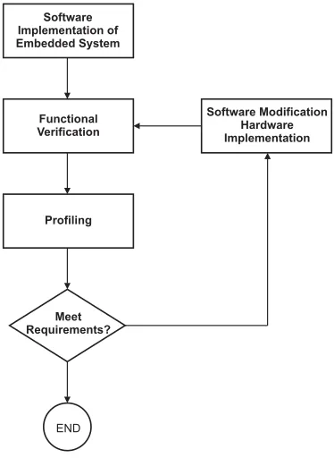
mance of the application code running on the target processor of an embedded system. Embedded designers have two options for the initial implementation of their design. First, the embedded system can be implemented entirely in hardware then moving certain components to the software domain, depending on the execution perfor-mance of those functions [25]. Second, the embedded system design can be implemented entirely in software [26] and then the software code is profiled using a profiler. It is used to detect any computational intensive portions in the code and other performance bottlenecks. The in-formation provided by the profiler is used by designers to help them choose which software functions are more desirable for hardware implementation and acceleration. The goal is to find an optimized partition of the embedded system based on the accurate profiled information such that it creates a proper balance between the hardware and software components in order to attain a speed-up in the overall system performance. This latter approach has led to a proposed Software Profiling Methodology (SPM) as shown in Figure 1 [13].

(3)

Profiling Tools

Software-Based Hardware-Based FPGA-Based

GNU’s gprof Valgrind Vtune Performance Analyzer

Hardware Counters Page Migration Approach

SnoopP Frequent Loop Analysis Tool

WOoDSToCK Airwolf

Figure 2. Classification of Profiling Tools

domain as a hardware accelerator. If necessary, the entire methodology starts again until the designer is satisfied with the performance.

Existing profiling tools offer different types of profiling capabilities and support different programming languages. C/C++ profiling tools are common, but there are also tools available that can profile programs written in Java [28]. Currently, there are many different kinds of profiling tools that are used to retrieve a variety of profiled information about a program. The most common is function-level profiling which measures the amount of time needed for a function to execute on the processor. Another type is memory profiling, provided by Rational Purify [29] and

Valgrind [30]. These memory profiling tools determine

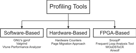
which function, data variable type or instruction is causing memory related problems: excessive memory references, cache misses, heavy pointer dereferencing, branching and looping instructions. Figure 2 shows a proposed classifi-cation of the existing profiling tools [31].

There are three main categories of profiling tools: software-based, hardware-based and FPGA-based. In this paper we discuss these categories.

A. Software-Based Profiling Tools

Software-Based Profiling (SBP) is the most common technique for measuring the performance of application code written in a programming language. There are two approaches to profiling the software code when using these tools: simulation and the insertion of instrumenta-tion code. Simulainstrumenta-tions take place in virtual environments that simulate the behaviour of a microprocessor as the software code is running in a virtual environment. The insertion of instrumentation code allows an SBP tool to attach itself to the binary file and collect performance information during the execution of a program on the processor. In this section, a description of the ISS and GNU’s gprof is given.

Instruction Set Simulators (ISS) are one of the SBP

tools used for profiling software code running in a simu-lated environment. One popular ISS is the SimpleScalar

Toolset which simulates application code running on the SimpleScalar computer architecture [32]. The advantages

of using an ISS for profiling is that the designer is able to view the entire data flow movement inside the micropro-cessor’s registers during the simulation. It keeps track of all of the execution processes, the current instruction in execution, data manipulations, cache accesses and other reportable events. This does not require the software code

to be modified, therefore intrusiveness to the binary file is non-existent.

The use of an ISS may not be feasible for larger software programs or with system-on-a-chip designs since they can be very slow to simulate [33]. This could lead to very inaccurate profiles of the execution times of each function. Simulations can have varying times to complete depending on the complexity of the software code. It may take several hours to run an entire simulation which may only cover a few seconds of real-time, thus misrepre-senting the entire execution time. Due to the increasing complexity of embedded systems designs, constructing complex models of the system’s components and other external environments may not be possible.

gprof [21] is an open-source profiling tool that is used

on Linux [34] and Unix [35] workstations to profile C and C++ application code. It provides two types of profiled outputs: the flat profile and the call graph. The flat profile is a report of how much time the program is spent on each function and the number of times that function was called. The call graph displays each function, its calling function and other functions called within that function. To utilize this profiler, the designer is required to the compile code with the default debug instrumentation setting. This option inserts additional instrumentation code into the binary executable file, as required by gprof.

During program execution, gprof utilizes the inserted instrumentation code to monitor the performance of the program running on the CPU. The instrumentation code allows gprof to count the precise number of function calls and generate the appropriate number of interrupts to sample the program counter (PC) of the CPU. It is capable of generating a profile that accurately counts the number of functions that have been called, however, the reported execution time of each function may be somewhat inaccurate.

gprof collects information on the execution time of a

program by reading the value of the PC at specified in-tervals. The PC value determines which function is being executed on the processor. Based on this value, gprof increments the execution time counter of the function that is currently executing by its sampling period. This can create inaccurate timing results for each function called and the execution time of the entire program [36]. The accuracy of the profiled execution time is entirely dependent on the sampling frequency of the PC.

(4)

unpredictable behaviour of the software code running on the embedded hardware platform. Additionally, the instrumentation code can lead to an increase in code size and may potentially change the behaviour and the performance of the software system.

B. Hardware-Counter Based Profiling (HCBP) Tools

Hardware-Counter Based Profiling (HCBP) tools utilize on-chip hardware counters that are available on advanced processors such as Sun Ultrasparc [37], Intel Pentium

Processors [38] and Advanced Micro Device (AMD)

Processors [39]. These hardware counters are dedicated to monitoring specific events that occur during runtime execution of an application. The types of events which can be monitored are: memory accesses, cache misses, pipeline stalls, types of instructions executed and etc. HCBP tools do not require the use of instrumentation code since these counters are designed to collect performance information of the software program. In addition, very little performance overhead is introduced during runtime execution.

Accessing these counters requires a unique instruc-tion. The Performance Advanced Programming Interface (PAPI) [40] provides users with a high level interface to access these counters and can supports many different processors [41]. Intel’s VTune counter monitor provides an interface for accessing and utilizing the hardware counters to profile application code executing on Pentium-based processors [38].

Itzkowitz et al from Sun Microsystems have described a

software profiling tool that utilizes the hardware counters in an Ultrasparc-III microprocessor [42]. Originally this profiling tool was built as an extension of the Sun One Studio [43] compilers and performance tools, which are used for measuring the performance of software code. These hardware counters are included in the ar-chitecture and contain different types of event counters such as, Instructions Completed, Instruction-cache (I$)

Misses, Data-cache (D$) Read Misses, Data-translation-lookaside-buffer (DTLB) Misses, External-cache (E$) References, E$ Read Misses, E$ Stall Cycles, and many

others.

There are some limitations to using this tool. One such limitation is counter-skidding [42]. The tool uses hardware-counter overflows to obtain profiled informa-tion. When a counter overflow occurs, the tool does not execute a precisely timed trapping mechanism to obtain the correct value of the counter. The second problem is the backtracking mechanism of instructions which was implemented as a solution to solve the trapping mech-anism flaw. The backtracking technique is used to find the instruction address that caused the overflow event to occur, however the instruction immediately preceding the current one in the processor’s PC may not have the correct address value, due to the possibility that the previous instruction was a branch call. Instead of relying on the value of the PC, the profiling tool tries to find the proper values in other registers to calculate the effective address

Sun Fire Link Hardware Counters

Processor #1 Memory

Physical Page

Processor #2 Memory

Physical Page

Processor #4 Memory

Physical Page Processor #3

Memory

Physical Page

Software Application

Page Migration

T

ransaction Sampling

Figure 3. Page Migration Approach

of the instruction that caused the overflow event. It is not guaranteed success in finding the address since the value of the registers may have changed once other overflow signals have been delivered to other hardware counters. Despite with these drawbacks, the tool has managed to find the proper instruction 99% of the time. The MCF benchmark was profiled and the feedback provided enabled a 20% performance improvement.

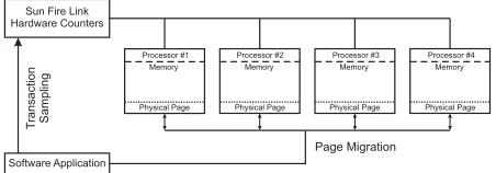
The Page Migration Approach (PMA), developed by

Tikir et al utilizes hardware-counters for profiling memory

with memory page-migrating capabilities [44]. The pro-filer was used on a multi-processor system based on Sun’s

SunFire Server as shown in Figure 3. Each system board

contained several processors and memory. The Sun Fire

Link hardware counters are used to sample the frequency

with which each processor “touches” a page of memory that is remote from the on-board local memory hardware. At a certain number of counts specified by the user for remote touching of memory pages, the profiler halts the execution. It then migrates that particular memory page to the processor that accesses it most frequently for read and write operations. PMA has demonstrated 90% speed improvement when certain memory pages are placed closest to the processor that requires data from that page.

There are consumer desktop processors today that contain hardware counters which monitor the performance of application code in the CPU. AMD Athlon micropro-cessors [39] contain four 48-bit performance hardware counters that can be used as event driven or timing driven counters. These counters can monitor the number of times a certain event occurs or they can measure the duration of an event that is currently taking place on the processor. Intel Pentium microprocessors also contain a set of performance hardware counters [38]. They are also event or timing driven and are accessible through Intel’s

VTune [45] profiling tool.

(5)

the hardware counters which leads back to the problems that were introduced with SBP tools. Thirdly, handling of interrupts affect the gathered data since the interrupt service routines (ISR) used add to the number of events. Lastly, there is a limited number of hardware counters available. The programmer must run the application many times to obtain data for different monitoring events [41].

C. FPGA-Based Profiling Tools

FPGA embedded development kits are a popular re-configurable design platform for synthesizing and rapid-prototyping of embedded systems. This is due to the con-tinuing advancement of FPGAs by providing increased logic capacity and other on-chip resources. FPGA-based embedded systems usually consist of a soft-core processor which is used as the target processor to execute software programs. The two major FPGA vendors, Altera [16] and Xilinx [17], provide embedded system development kits that uses Nios II [23] and MicroBlaze [19] soft-core processors respectively. These processors are instantiated in the embedded system design, in which they are used as basic building blocks for the design of embedded systems [10], [15].

FPGA-based profiling (FPGA-BP) tools also utilize these soft-core processors for profiling. In FPGA-BP tools, the designer executes the software on the soft-core processor and collects the performance data provided by the on-chip profiling hardware. These tools have provided improved results compared to the previous profiling tools described earlier. They keep latency and performance overhead at a minimum, because they are non-intrusive and require negligible instrumentation. They do not use the sampling technique and require very minimal pro-cessor computation. These features are highly desirable for profiling tools used in embedded systems. In this section, a detailed discussion of the proposed FPGA-based profiling tools to date is provided.

SnoopP [13] is an on-chip function level profiler that

was implemented on the Xilinx Virtex-II 2000 FPGA board. This board is used to implement designs based on the Xilinx MicroBlaze soft processor [19]. The on-chip profiler utilizes the MicroBlaze as a target processor.

SnoopP uses a hardware profiling architecture that is

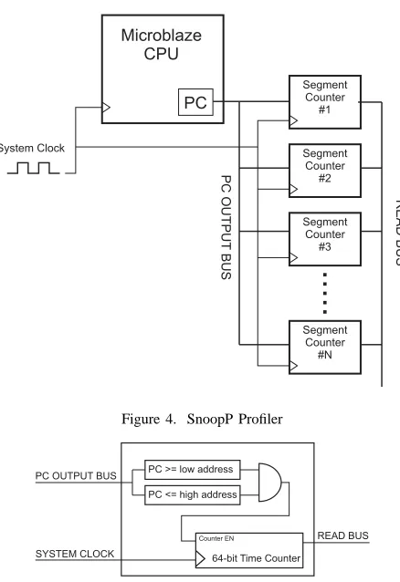
non-intrusive to the code, such that any additional instructions, commands or other flags are not necessary. Figure 4 depicts the hardware architecture for the SnoopP profiler. As shown in Figure 4, SnoopP consists of a variable number of segment counters that are user specified and define the address of instructions to be analyzed. The number of segment counters is dependent on the number of functions the user wishes to profile and the area available on the FPGA.

The comparators inside SnoopP’s profiling counters, shown in Figure 5, determine if the value of the PC address is in the range of memory addresses in which the binary code corresponding to the function resides. This is determined by the comparators inside each segment counter. If this condition is true, the comparator sends an

Microblaze CPU

PC

Segment Counter

#1

Segment Counter

#2

Segment Counter

#3

Segment Counter

#N

...

System Clock

PC

OUTPUT

BUS

READ

BUS

Figure 4. SnoopP Profiler

PC >= low address

PC <= high address

64-bit Time Counter

Counter EN

PC OUTPUT BUS

SYSTEM CLOCK

READ BUS

Figure 5. SnoopP’s Profiling Counter

enable signal to the hardware counter which utilizes the processor’s system clock to count the number of clock cycles the function has used. This gives the designer the precise number of clock cycles that the particular function needs to execute on the processor. SnoopP’s and gprof ’s results were compared, and it was shown that SnoopP was significantly more accurate. Additionally, SnoopP does not slow down the performance of either the software or the profiling process.

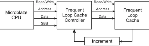
Frequent Loop Analysis Tool (FLAT) is a tool that

detects functions in software that heavily use loops [46]. In most cases, loops use 90% of the execution time while constituting only 10% of the entire software code. FLAT searches for these critical regions and records the execution frequency of each loop-intensive function into a cache-like hardware architecture that is implemented on an FPGA. A block diagram of the FLAT architecture is shown in Figure 6.

Usually a loop instruction is typically denoted as a short backwards branch (SBB), when the program jumps back to the first instruction of that loop. The value of the SBB is a negative address offset. The Frequent Loop

Cache (FLC) stores the execution frequency of each loop

(6)

Microblaze CPU

Frequent Loop Cache

Controller

Read/Write

Address

Data

SBB

Read/Write

Address

Data

Frequent Loop Cache

Increment

Figure 6. Frequent Loop Analysis Toop

WOoDSTOCK [47] (Watches Over Data STreaming

On Computing element linKs), is a profiling tool that

monitors the communication dataflow between Comput-ing Processor Elements (CPEs). It helps determine the components that cause communication bottlenecks in the entire system.

WOoDSToCK monitors the data flow between each CPE by adding monitors to the circuit which run in real time. The data link between each element of the system is created by Fast Simplex Links (FSLs) [48], available in Xilinx’s MicroBlaze [19] soft-core processor. FSLs allow streaming and buffering of data between the hardware components of the system. The profiler utilizes the links to measure the stream of data between each CPE. It measures the number of run-time execution clock cycles to see which CPE is stalled or starved for data.

A stalled CPE occurs when a stream of data is at the input but little or no output data is coming out. A starved computing element occurs when little data is coming in or going out of the CPE, but it is still running. The results obtained showed that the tool was able to detect bottlenecks using a pipelined system and a branching system benchmark.

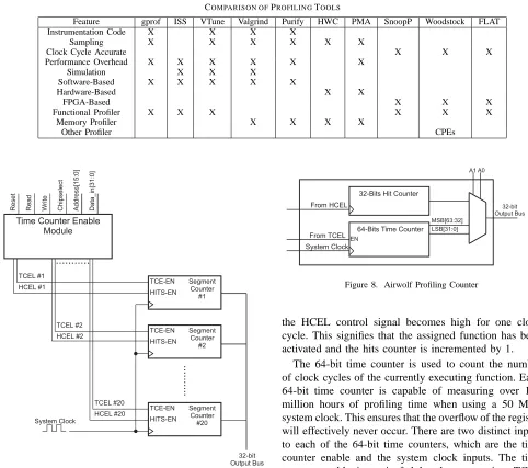
D. Qualitative Comparison of Profiling Tools

There are a variety of profiling tools available today that can measure the performance of software code by col-lecting information about different performance metrics. The majority of these tools have one or more drawbacks related to accuracy, runtime overhead and extended exe-cution time. Table I shows a comparison of the profiling tools discussed in this paper.

The SBP tools have functional and memory profiling capabilities. They do require the insertion of code that is needed to interrupt the processor at specific intervals to sample the data stored in the hardware registers in the system. This can cause inaccurate profiled results reported along with the introduction of performance overhead during execution and an increase in file size. This is not desirable in the design of embedded systems.

One of the advantages of using simulators is that the original program does not require any insertion of code. This is beneficial since this does not modify the behaviour of the software program, although simulating large programs is very slow and is therefore an impractical option for profiling large embedded system designs.

HCBP tools are mostly used for profiling memory systems, however, they do use techniques that are similar to those used by software-based profiling tools, such as

sampling, which can affect the accuracy of the perfor-mance information retrieved. The accuracy of the profiled results is dependent on the frequency of the sampling rate. FPGA-BP tools are clock-cycle accurate and do not introduce overhead during software execution. The soft-ware program may require minimal code disturbance or can be left alone, thus reducing the effect of unpredictable execution behaviour. We can observe from the table that FPGA-BP tools are not as restricted as functional or memory profilers. They also have the ability to detect communication bottlenecks between CPEs.

III. THEAIRWOLFPROFILER

The Airwolf Profiler is an on-chip FPGA-BP tool used to profile software programs running on the Nios II [23] Processor in real-time. This is done by determining the run-time of each software function by accurately counting the number of system clock cycles. The modification of the interface of the Airwolf Profiler can also be instantiated on other embedded soft-core processors such as Tensilica Xtensa Soft-Core Processor [49] and the Xilinx MicroBlaze Soft-Core Processor [19]. Airwolf does not require any instrumentation code added to the binary file. A pair of software drivers needs to be placed in between a software function block in the source code in order to activate and deactivate a particular profiling counter contained in Airwolf. This approach minimally disturbs the program and the software behaviour during execution. The goal of the Airwolf Profiler is to provide accurate results while minimally modifying the software code. Figure 7 depicts the Airwolf Profiler Architecture.

A. Airwolf Profiling Architecture

As shown in the figure, the Airwolf Profiler con-tains the Time Counter Enable (TCE) module and 20 profiling counters. This is sufficient for profiling large programs that consist of a large number of software func-tions. Instantiating the Airwolf Profiler onto the Stratix EP1S40F780C5 FPGA [50] consumes 3,345 logic ele-ments. The maximum operating frequency of this profiler is 120 MHz. Hence, this can be used for high-speed Nios II Processor systems [23].

The TCE module contains 20 Counter Enable (CE) registers which are used to activate the appropriate pro-filing counter. The logic circuit in the TCE module is dependent on the Address and Data In bus inputs that are being fed from the Avalon Interface Bus (AIB) [51]. The AIB contains all of the necessary control logic signals that are used to manipulate the CE registers in the TCE module. The accompanying software drivers of the Airwolf Profiler are programmed to access the appropriate CE register by sending a unique address onto the interfacing bus. The output of each CE register is fed into the input enable of the assigned profiling counter (shown as the Time Counter Enabling Lines (TCELs) in the figure).

(7)

TABLE I.

COMPARISON OFPROFILINGTOOLS

Feature gprof ISS VTune Valgrind Purify HWC PMA SnoopP Woodstock FLAT

Instrumentation Code X X X X

Sampling X X X X X X

Clock Cycle Accurate X X X

Performance Overhead X X X X X X

Simulation X X X

Software-Based X X X X X

Hardware-Based X X

FPGA-Based X X X

Functional Profiler X X X X X X

Memory Profiler X X X X

Other Profiler CPEs

Time Counter Enable Module

Segment Counter

#1 TCE-EN HITS-EN

Segment Counter

#2 TCE-EN HITS-EN

Segment Counter #20 TCE-EN HITS-EN

...

TCEL #1

HCEL #1

TCEL #2 HCEL #2

TCEL #20 HCEL #20 ...

Reset Read Write Chipselect Address[15:0] Data_in[31:0]

System Clock

32-bit Output Bus

Figure 7. The Airwolf Profiler

is to indicate when a function has been called as the program is executing on the processor.

The Data In and Address input buses are also used to extract the profiling data stored in the profiling counters. These data are sent out to a host computer through the

Data Out bus. A set of control signals provided by the

AIB, namely the chipselect, write enable and read enable signals, are used to prevent any illegal input or output accesses of the CE registers and the profiling counters.

B. Airwolf Profiling Counter

The Airwolf Profiler contains 20 profiling counters which allow for up to 20 functions to be profiled at a time. Figure 8 depicts the contents of each profiling counter.

Each profiling counter actually consists of two coun-ters, a 32-bit hits counter and a 64-bit time counter. The hits counter counts the number of positive edges of the input HCEL control signal. When the appropriate profiling software driver activates the profiling counter,

EN From TCEL

From HCEL

MSB[63:32]

LSB[31:0]

SystemClock

A0 A1

32-bit OutputBus

32-Bits HitCounter

64-BitsTimeCounter

Figure 8. Airwolf Profiling Counter

the HCEL control signal becomes high for one clock cycle. This signifies that the assigned function has been activated and the hits counter is incremented by 1.

The 64-bit time counter is used to count the number of clock cycles of the currently executing function. Each 64-bit time counter is capable of measuring over 100 million hours of profiling time when using a 50 MHz system clock. This ensures that the overflow of the register will effectively never occur. There are two distinct inputs to each of the 64-bit time counters, which are the time counter enable and the system clock inputs. The time counter enable input is fed by the appropriate TCEL control line, which controls the counting sequence of the counter. If the TCEL signal becomes high and remains at that state, the counter begins to count the number of positive edges of the system clock. If the TCEL signal becomes low, counting of the clock ticks is disabled. This concept is of great importance since Airwolf accurately counts the number of clock ticks a function has taken. This helps to provide accurate performance feedback which can be beneficial for embedded system designers. A multiplexer component that is controlled by the address bits from the Address input bus exists in every profiling counter. This mandates which data is assigned to the AIB. In the end, the profiled data stored in these counters is extracted by calling the appropriate software driver and displayed for the designer.

IV. PROFILINGENVIRONMENT ANDBENCHMARKS

(8)

TABLE II.

NIOSDEVELOPMENTBOARDCOMPONENTS

Nios Development Board

Stratix Professional Edition 41250 Logic Elements Static RAM (Off-Chip) Module 1MB

Flash Ram (Off-Chip) Module 8MB

UART

Controller

SRAM/Flash

Memory Controller

System Clock Timer

High Resolution

Timer

Airwolf Profiler NiosII/Fast

Processor Core

64KB I-Cache

64KB D-Cache Hardware MUL/DIV

A

valon

Interface

Bus

Inst.

Data

Figure 9. Nios II Profiling Environment

A. Profiling and Design CAD Tools

The two profiling tools, Nios2-gprof and the Airwolf Profiler were utilized in measuring the performance of the software code running on the soft-core processor, Nios II. A Nios II Processor System was built as the target hardware platform that was used for running and profiling software programs. We refer this as the Nios II

Pro-filing Environment (Nios-II-PE). Nios2-gprof is Altera’s

implementation of the GNU’s gprof profiler. The Airwolf Profiler is the FPGA-based profiler that is a component of the Nios-II-PE. The following design tools were used for this experiment: Altera’s Quartus II Version 5.0 SP2 [52], Nios II IDE Version 5.0 [53] and SOPC Builder Version 5.0 [54].

B. FPGA Development Board

The Nios Development Kit [24] was used to implement the Nios-II-PE. This kit contains a Nios Development Board, Stratix Professional Edition, featuring a Stratix EP1S40F780C5 FPGA chip. The chip features 41,250 logic elements, 3,423,744 memory bits and 14 Digital Signal Processing (DSP) blocks, [50]. There are available off-chip memory modules that can be used, which include the 8MB flash memory, the 1MB SRAM and the 16MB SDRAM modules. In this experiment, the 1MB SRAM was used for the program, stack and data memories for each benchmark. All of the components on the develop-ment board utilized the 50MHz clock oscillator as the system clock of the Nios-II-PE.

C. Nios II Profiling Environment

Figure IV-C shows the diagram of the profiling envi-ronment, namely the Nios-II-PE, and Table IV lists the instantiated Intellectual Property (IP) cores. The Nios-II-PE consists of the fast version of the Nios II Processor core, which is a soft-core processor that is optimized

TABLE IV.

NIOSII PROFILINGENVIRONMENTCOMPONENTS

Nios II Profiling Environment

Nios II Fast-Core Processor (with Hardware Multiply/Divide) 1MB SRAM Controller

System Clock and High Resolution Timers UART Controller

The Airwolf Profiler

for high performance in computationally-intensive ap-plications at the expense of consuming more logic ele-ments on an FPGA [23]. This processor is suitable for executing the benchmarks used in this experiment. The core contains multiply and divide hardware accelerators which allow multiplication and division operations to be executed in hardware. In addition, it contains separate instruction and data cache memories, each having 64KB. For the program, stack and data memories, the Nios-II-PE utilizes the 1 MB static Random Access Memory (RAM) module which is located off-chip. Software benchmarks are downloaded onto this memory module. There are two timers in this system, namely the system clock and high performance timers. They are required for Nios2-gprof in order to measure the run-time of the software functions and by some of the software benchmarks as well. An instance of the Airwolf Profiler is used in the Nios-II-PE, consisting of all 20 profiling counters. Each of these counters is assigned a specific software function to profile. The Universal Asynchronous Receiver and Transmitter (UART) controller is used to communicate with the Nios-II-PE and to transfer streaming messages back to the host computer. All of the instantiated components in the Nios-II-PE are connected using the Avalon Interface Bus (AIB) [51] which provides all of the necessary control logic and data signals that are used to communicate between each instantiated component.

D. Software Benchmarks

The profiling software benchmarks used in this ex-periment are listed in Table III, along with a brief description of each. These benchmarks were obtained from MiBench [55], [56] and the UTNiosbenchmarks [57]. Each benchmark was compiled using the Nios II GCC compiler applying the highest optimal compilation (-O3) setting. The compiler generates the executable binary by optimizing the code for fast performance at the expense of a slightly larger file size [58].

Each benchmark was slightly modified for each of the profile runs so that no function calls any other function in the program. The reported execution time is dedicated to the assigned function, and not to any other function that may be called.

(9)

TABLE III. BENCHMARKDESCRIPTIONS

Profiling Software Benchmarks

BitCount Performs several bit manipulations (10,000,000 iterations) Dhrystone Tests the integer performance of a microprocessor (100,000,000 iterations)

Dijkstra Computes the shortest path between 160 distinct nodes

Fibo Matrix Mult First computes the 40th Fibonacci term and then multiplies two 250x250 matrices

inserted in between each function. One driver is used to activate and the other to deactivate the assigned function’s profiling counter.

V. EXPERIMENTALRESULTS

Each benchmark was executed with Nios2-gprof and the Airwolf Profiler with their respective software compi-lation settings. In the subsequent paragraphs, we present an analysis of the profiled results for each of the bench-marks listed in Table III.

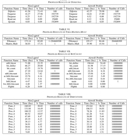
A. Dijkstra

Table V shows the profiled results for the Dijkstra benchmark. The first four columns show the results ob-tained by Nios2-gprof and and the latter four columns show the results obtained with Airwolf profilers. The first column gives the function name. The second column shows the execution time of each function. The third column shows the function’s execution as a percentage of total execution time of the benchmark. The number of function calls is displayed in the fourth column. The same explanation applies for the remaining columns in the table and for all subsequent tables.

Each profiler’s results are alike, having similar exe-cution times and rankings of computationally intensive functions. The Dijkstra function is reported to run for 41.56 seconds by Nios2-gprof whereas the Airwolf Profiler reported 42.27 seconds.

There are very minor differences in the reported ex-ecution times of the remaining software functions. This implies that Nios2-gprof reports results with comparable accuracy to those of the Airwolf profiler for smaller, less computationally intensive benchmarks. Airwolf attained an improvement in accuracy of 1.67%.

B. Fibo Matrix Mult

Table VI depicts the profiled results of the

Fibo Matrix Mult benchmark. Nios2-gprof reported that the Fibonacci function was called only once. The call-graph, however, displays that the function was recursively called 204,668,308 times. This explains the “+” in between the two values. Similarly, Airwolf reported that the number of calls to Fibonacci was 204,668,309. In terms of the run-time, Nios2-gprof and Airwolf reported that the function was running for 172.14 and 195.17 seconds respectively. This implies that the sampling technique used in Nios2-gprof has produced an inaccurate report of the execution time when profiling recursive function calls. In contrast, the

clock-cycle counting method that Airwolf utilizes shows an 11.79% accuracy improvement in the reported time for that function.

The Matrix_Mult function had very minor

differ-ence in the reported time between the two profilers. The percentage difference is 0.36%.

C. BitCount

Table VII shows the profiled results for the BitCount benchmark. There is a significant difference in the ported execution time of each function when the re-sults from each profiler are compared. Not only do the execution times differ, but Nios2-gprof also ranked the most time consuming functions differently than Airwolf.

Nios2-gprof listed the ntbl_bitcnt,bit_shifter

and bit_count as the most time consuming

func-tions, whereas the Airwolf Profiler reported that the

bit_shifter,bit_countandntbl_bitcnt

func-tions contributed the most toward the total execution time of the benchmark.

Nios2-gprof reported that bit_shifter ran for 66.27 seconds whereas Airwolf Profiler has measured that function to take 196.64 seconds on the processor. Once again, due to the sampling technique used by

Nios2-gprof, the profiler provided an inaccurate reporting of the

execution time. Airwolf Profiler provided up to 66.2% improvement in accuracy in some of the functions.

As for thentbl_bitcntfunction, which was called recursively, Nios2-gprof and Airwolf reported that the function was running for 71.88 and 51.34 seconds re-spectively. This shows that Nios2-gprof reports inaccurate execution times when profiling recursive functions.

Nios2-gprof reported that the btbl_bitcnt and

Flipbit functions were called during the execution of

the benchmark. However, the Airwolf Profiler did not detect calls to those functions. The insertion of instru-mentation code not only generates additional function calls and interrupts, but it can also cause unpredictable behaviour of the executing program.

D. Dhrystone

Table VIII shows the profiled results for the Dhrystone benchmark. Both profilers have similarly ranked the most time consuming functions. However, the reported execu-tion times of each funcexecu-tion were quite different.Proc_1 was reported to take 131.84 and 106.53 seconds by

Nios2-gprof and the Airwolf Profiler respectively. This amounts

to a 19.19% improvement in accuracy when using the

Airwolf Profiler. Another observation is with regards to

(10)

TABLE V.

PROFILEDRESULTS OFDIJKSTRA

Nios2-gprof Airwolf Profiler

Function Name Time (Sec) % Time Number of calls Function Name Time (Sec) % Time Number of Calls

Dijkstra 41.56 71.43 160 Dijkstra 42.27 70.98 160

Enqueue 16.27 27.96 192739 Enqueue 16.61 27.89 192739

Dequeue 0.25 0.43 192739 Dequeue 0.52 0.88 192739

Read int 0.05 0.09 25600 Read int 0.12 0.20 25600

Qcount 0.05 0.09 192899 Qcount 0.03 0.05 192899

TABLE VI.

PROFILEDRESULTS OFFIBOMATRIXMULT

Function Name Time (Sec) % Time Number of calls Function Name Time (Sec) % Time Number of Calls Fibonacci 172.14 82.69 1+204668308 Fibonacci 195.17 84.46 204668309

Matrix Mult 36.03 17.31 1 Matrix Mult 35.90 15.54 1

TABLE VII.

PROFILEDRESULTS OFBITCOUNT

Function Name Time (Sec) % Time Number of calls Function Name Time (Sec) % Time Number of Calls ntbl bitcnt 71.88 22.35 80000000 bit shifter 196.64 54.40 10000000

bit shifter 66.27 20.60 10000000 bit count 61.98 17.15 10000000 bit count 63.55 19.76 10000000 ntbl bitcnt 51.34 14.20 80000000

main 47.10 14.64 1 ntbl bitcount 22.26 6.16 10000000

ntbl bitcount 24.51 7.62 10000000 ar btbl bitcount 15.04 4.16 10000000 ar btbl bitcount 19.76 6.14 10000000 bitcount 12.63 3.49 10000000 bitcount 17.41 5.41 10000000 bw btbl bitcount 4.40 0.44 10000000

btbl bitcnt 6.47 2.01 main 0.01 0.00 1

bw btbl bitcount 4.40 1.37 10000000 btbl bitcnt 0.00 0.000

Flipbit 0.28 0.09 Flipbit 0.00 0.00

TABLE VIII.

PROFILEDRESULTS OFDHRYSTONE

Function Name Time (Sec) % Time Number of calls Function Name Time (Sec) % Time Number of Calls

Func 2 240.02 30.02 100000000 Func 2 253.64 38.32 100000000

Proc 1 131.84 16.49 100000000 Proc 1 106.53 16.01 100000000

Proc 8 100.52 12.57 100000000 Proc 8 78.26 11.83 100000000

Proc 6 80.52 10.07 100000000 Proc 6 62.28 9.41 100000000

Func 1 67.69 8.47 300000000 Proc 2 36.00 5.44 100000000

Proc 3 49.19 6.15 100000000 Func 1 34.69 5.24 300000000

Proc 7 38.13 4.77 300000000 Proc 7 30.14 4.55 300000000

Proc 2 36.91 4.62 100000000 Proc 3 22.13 3.34 100000000

Proc 4 30.01 3.75 100000000 Proc 4 18.00 2.72 100000000

Proc 5 15.11 1.89 100000000 Func 3 10.14 1.53 100000000

Func 3 9.69 1.21 100000000 Proc 5 10.00 1.51 100000000

reported that Func_1 took 67.69 seconds to execute

andProc_3ran for 49.19 seconds. However, the results

obtained with the Airwolf Profiler showed that Func_1 had an execution time of 34.69 and thatProc_3executed for 22.13 seconds. Again, a 55% improvement in accuracy was obtained using the Airwolf profiler.

VI. PERFORMANCEOVERHEADANALYSIS

Nios2-gprof requires the C/C++ file to be compiled

with instrumentation code which generates additional software interrupts and counter variables in the original program. This can lead to a large increase in the execution time of the benchmark and can cause an inconvenience to the embedded system designer who has to wait to retrieve the profiled results. This becomes a major impediment as the software code size grows larger.

In this section, an analysis of the performance overhead is presented for the software benchmarks discussed above. Each software program was compiled with the default debug (-g) setting while the same assigned functions were profiled with the Airwolf Profiler. The performance overhead was determined by summing the execution time of each profile run, with and without instrumentation code.

Table IX shows the performance overhead analysis for

Dijkstra. Column 1 lists the function names. Columns

2 and 3 show the execution times when the program was executing with and without instrumentation code respectively. The last column shows the time difference between the two compilation runs.

(11)

TABLE IX.

PERFORMANCEOVERHEADANALYSIS OFDIJKSTRA

Function Name Execution Time (Sec) Execution Time (Sec) with Instrumentation Difference (Sec)

Dijkstra 42.20 43.24 1.04

Enqueue 16.60 17.22 0.62

Dequeue 0.52 0.92 0.4

Read int 0.12 0.12 0

Qcount 0.031 0.031 0

Performance Overhead: 3.35%

TABLE X.

PERFORMANCEOVERHEADANALYSIS OFFIBOMATRIXMULT

Fibonacci 195.17 357.90 162.74

Matrix Mult 35.90 36.00 0.10

TABLE XI.

PERFORMANCEOVERHEADANALYSIS OFBITCOUNT

bit shifter 196.64 197.31 0.67

bit count 61.98 62.18 0.20

ntbl bitcnt 51.34 99.77 48.43

ntbl bitcount 22.26 22.31 0.05

AR btbl bitcount 15.04 15.09 0.05

bitcount 12.63 12.66 0.03

BW btbl bitcount 1.60 1.60 0.00

btbl bitcnt 0.00 0.00 0

TABLE XII.

PERFORMANCEOVERHEADANALYSIS OFDHRYSTONE

Func 2 253.64 361.23 107.59

Proc 1 106.53 106.00 -0.53

Proc 8 78.26 83.00 4.74

Proc 6 62.28 130.00 67.72

Proc 2 36.00 37.59 1.59

Func 1 34.69 33.00 -1.69

Proc 7 30.14 30.00 -0.14

Proc 3 22.13 25.00 2.87

Proc 4 18.00 18.25 0.25

Func 3 10.14 10.00 -0.14

Proc 5 10.00 10.00 0.000

on smaller benchmarks, such as Dijkjstra, contributes minimal performance overhead. In this case, only 3.35% of additional execution time was contributed by the in-strumentation code.

Table X depicts the performance overhead analysis for the Fibo Matrix Mult benchmark. Notice that the

Fibonacci function has taken 162.74 seconds of

ad-ditional execution time. The added instrumentation code changed the behaviour of the software benchmark. Since

the Fibonacci function was called recursively, this

implies that instrumentation code adds significant perfor-mance overhead when profiling recursive functions with

Nios2-gprof. This has caused the entire benchmark to have

a performance overhead of 41.34%

Table XI demonstrates the performance overhead analy-sis for the BitCount benchmark. The instrumentation code added an additional 48.43 seconds in execution time to the recursively called function ntbl_bitcount. This strongly supports the idea that profiling recursive

func-tions with Nios2-gprof can cause a significant increase in run-time execution. The other functions listed in this table show minor differences in the execution time. This has resulted an overall performance overhead of 12.10%.

Table XII depicts the execution time differences of each software function in Dhrystone. Some of the functions showed a slight decrease in execution time, resulting in the negative time differences shown in the table. This is probably caused by the inserted instrumentation code that changes the normal behaviour of those functions during execution. This could potentially give inaccurate reporting from Nios2-gprof. Since those negative values are diminutive however, it minimally affects the en-tire benchmark’s execution time. The software functions

Func_2andProc_6show a significant increase in

(12)

VII. CONCLUSIONS ANDFUTUREWORK In this paper, we presented a detailed discussion and comparison of different profiling tools for FPGA-based embedded systems. We described Airwolf, an FPGA-based profiling tool developed for Altera Nios II [23] based embedded systems. We described an experimen-tal framework, called the Nios II Profiling Environment (Nios-II-PE), that was used for profiling a set of soft-ware benchmarks using softsoft-ware-based and FPGA-based profilers, namely Nios2-gprof and the Airwolf Profiler respectively. Experimental results show that the Airwolf Profiler provides up to a 66.2% accuracy improvement. This is beneficial to embedded system designers since they rely on accurate performance information to imple-ment the appropriate software functions in the hardware domain. Nios2-gprof uses the sample technique which has a tendency to report inaccurate timing of each function in the software code. The Airwolf Profiler counts the number of clock ticks that each function uses which provides an accurate report of the execution time of each function.

The performance overhead analysis has also shown further disadvantages when profiling with SBP tools. Adding instrumentation code at the binary level not only is intrusive but has caused computationally intensive functions to run longer than normal. In some of the soft-ware benchmarks, the instrumentation code has caused a performance overhead of up to 41.3%. This added time and overhead is unnecessary since it causes Nios2-gprof to report inaccurate execution times of each function and longer delays for the designer to retrieve the profiled results.

The Airwolf Profiler was designed for research pur-poses to profile software applications running on an Altera Nios II processor implemented on an Altera FPGA. It can easily be modified to become an instruction address-based profiler that has the capability to monitor the current instruction in execution on the processor. This concept can provide an improvement in the profiled results compared to the current software driver strategy. In future work, the

Airwolf Profiler can be enhanced to cover memory

profil-ing as well, which monitors memory related events such as the number of off-chip memory accesses, cache misses and memory leaks. This can further benefit embedded system designers and help in improving certain portions of the software code that cause memory related performance issues. The Airwolf profiler can also be easily modified to work with other FPGA-based soft core processors such as Xilinx’s MicroBlaze [19].

ACKNOWLEDGMENT

The authors would like to thank the Altera Corpora-tion for their generous equipment and software support. Thanks are also due to Lisa Price and Ian Anderson for their invaluable comments and suggestions.

REFERENCES

[1] W. Wolf, “A Decade of Hardware/Software Co-Design,” in

Proc. of the 5th International Symposium on Multimedia Software Engineering (MSE2003), Dec. 2003, pp. 38–43.

[2] K. Keutzer, S. Malik, A. R. Newton, M. Rabaey, and A. Sangiovanni-Vincentelli, “System-Level Design: Or-thogonalization of Concerns and Platform-Based Design,”

IEEE Transactions on Computer Aided Design for Inte-grated Circuits and Systems, vol. 19, no. 12, pp. 1523–

1542, December 2000.

[3] P. Pop, P. Elese, and Z. Peng, Analysis and Synthesis of

Distributed Real-Time Embedded Systems, 1st ed. The Netherlands: Kluwer Academic Publishers, 2004. [4] G. E. Moore, “Cramming More Components onto

Inte-grated Circuits,” Proceedings of the IEEE, vol. 86, no. 1, pp. 82–85, January 1998.

[5] K. Compton and S. Hauck, “Reconfigurable Computing: A Survey of Systems and Software,” ACM Computing

Surveys, vol. 34, no. 2, pp. 171–210, June 2002.

[6] I. Amer, W. Badawy, and G. Jullien, “A Design Flow for an H.264 Embedded Video Encoder,” in Proc. of the 3rd

International Conference on Information and Communica-tions Technology, November 2005, pp. 178–181.

[7] T. Wiangtong, P. Y. K. Cheung, and W. Luk, “Hard-ware/software Codesign: A Systematic Approach Target-ing Data-intensive Applications,” IEEE Signal ProcessTarget-ing

Magazine, vol. 22, pp. 14–22, May 2005.

[8] S. Ha, C. Lee, Y. Yi, S. Kwon, and Y.-P. Joo, “Hardware-Software Codesign of Multimedia Embedded Systems: the PeaCE Approach,” in Proc. of the 12th IEEE International

Conference on Embedded and Real-Time Computing Sys-tems and Applications, August 2006, pp. 207–214.

[9] P. Schaumont, D. Ching, and I. Verbauwhede, “An in-teractive Codesign Environment for Domain-Specific Co-processors,” ACM Transactions on Design Automation of

Electronic Systems, vol. 11, pp. 70–87, January 2006.

[10] N. Ohba and K. Takano, “An SoC Design Methodology using FPGAs and Embedded Processors,” in Proc. of the

41st Annual Conference on Design Automation, June 2004,

pp. 747–752.

[11] S. A. Edwards, “Experiences Teaching an FPGA-based Embedded System Class,” in Proc. of the 1st Workshop

on Embedded System Education, vol. 2, October 2005, pp.

56–62.

[12] G. Stitt, R. Lysecky, and F. Vahid, “Dynamic Hard-ware/Software Partitioning: A First Approach,” in Proc.

of the 40th Conference on Design Automation, June 2003,

pp. 250–255.

[13] L. Shannon and P. Chow, “Using Reconfigurability to Achieve Real-Time Profiling for Hardware/Software Code-sign,” in Proc. of the 12th International Symposium on

Field Programmable Gate Arrays, February 2004, pp. 190–

199.

[14] R. Lysecky and F. Vahid, “A Study of the Speedups and Competitiveness of FPGA Soft Processor Cores using Dynamic Hardware/Software Partitioning,” in Proc. of the

Conference on Design, Automation and Test in Europe (DATE), March 2005, pp. 18–23.

[15] J. G. Tong, I. D. L. Anderson, and M. A. S. Khalid, “Soft-Core Processors for Embedded Systems,” in Proc.

of the 18th International Conference on Microelectronics,

December 2006, pp. 170–173.

[16] Altera Corporation. [Online]. Available:

http://www.altera.com

[17] Xilinx Incorporated. [Online]. Available:

http://www.xilinx.com

[18] Z. Guo, W. Najjar, F. Vahid, and K. Vissers, “A Quan-titative Analysis of the Speedup Factors of FPGAs over Processors,” in Proc. of the 12th International Symposium

on Field Programmable Gate Arrays, February 2004, pp.

162–170.

(13)

[20] J. G. Tong and M. A. S. Khalid, “A Comparison of Profiling Tools for FPGA-based Embedded Systems,” in

Proc. of the 20th Canadian Conference on Electrical and Computer Engineering, April 2007, pp. 1687–1690.

[21] J. Fenlason and R. Stallman, GNU

gprof, January 1997. [Online]. Available: http://www.gnu.org/software/binutils/manual/gprof-2.9.1/ [22] Performance Counter Peripheral, Altera Corporation,

November 2005.

[23] Nios II Processor Handbook, Altera Corporation, October 2005.

[24] Altera Corporation, Accessed

De-cember 2006. [Online]. Available:

http://www.altera.com/products/devkits/altera/kit-nios 1S40.html

[25] R. K. Gupta and G. DeMicheli, “Hardware-Software Cosynthesis for Digital Systems,” IEEE Transactions on

Design and Test of Computers, vol. 10, pp. 29–41,

Septem-ber 1993.

[26] R. Ernst, J. Henkel, and T. Benner, “Hardware-Sotware Cosynthesis for Microcontrollers,” IEEE Transactions on

Design and Test of Computers, vol. 10, no. 4, pp. 64–75,

December 1993.

[27] C. J. N. Coelho Jr., D. C. DaSilva Jr., and A. O. Fernandes, “Hardware-Software Codesign of Embedded Systems,” in

Proc. of the 11th Brazilian Symposium on Integrated Circuit Design, January 1998, pp. 2–8.

[28] J. Fleishmann and K. Buchenrieder, “Codesign of Embed-ded Systems Based on Java and Reconfigurable Hardware Components,” in Proc. of the Design, Automation and Test

in Europe Conference and Exhibition, March 1999, pp.

768–769.

[29] Rational PurifyPlus, Rational Purify, Rational Pure

Cov-erage, Rational Quantify. Installing and Getting Started. Version 2003.06.00, Technical White Paper.

[30] Valgrind, Accessed October 2006. [Online]. Available: http://www.valgrind.org

[31] J. G. Tong and M. A. S. Khalid, “Profiling CAD Tools: A Proposed Classification,” in Proc. of the 19th International

Conference on Microelectronics, December 2007, pp. 253–

256.

[32] D. Burger and T. M. Austin, “The SimpleScalar Tool Set Version 2.0,” ACM SIGARCH Computer Architecture

News, vol. 25, no. 3, pp. 13–25, June 1997.

[33] R. Lysecky, S. Cotterell, and F. Vahid, “A Fast On-Chip Profiler Memory,” in Proc. of the 39th Conference on

Design Automation, June 2002, pp. 28–33.

[34] The Linux Homepage. [Online]. Available:

http://www.linux.org

[35] The Unix System. [Online]. Available: http://www.unix.org [36] D. A. Varley, “Practical Experience of the Limitations of gprof,” in Software Practice and Experience, 1993, pp. 461–463.

[37] Sun Microsystems, Using UltraSPARC-IIICu Performance

Counters to Improve Application Performance,

Accessed February 2006. [Online]. Available:

http://developers.sun.com/prodtech/cc/articles/pcounters.html

[38] Intel Corporation, IA-32 Intel Architecture

Software Developer’s Manual, Accessed

February 2006. [Online]. Available:

http://developers.sun.com/prodtech/cc/articles/pcounters.html [39] AMD Athlon Processor, x86 Code Optimization Guide,

2002.

[40] S. Brown, S. Browne, J. Dongarra, N. Garner, K. London, and P. Mucci, “A scalable cross-platform-infrastructure for application performance tuning using hardware-counters,” in Proc. of the 2000 ACM/IEEE conference on

Supercom-puting, 2000.

[41] B. Sprunt, “The Basics of Performance-Monitoring

Hard-ware,” IEEE Micro, vol. 22, no. 4, pp. 64–71, July-August 2002.

[42] M. Itzkowitz, J. N. W. Brian, C. Aoki, and N. Kosche, “Memory profiling using hardware counters,” in Proc. of

the 2003 ACM/IEEE conference on Supercomputing, July

2003, pp. 17–30.

[43] Sun One Studio 5, Standard Edition, Sun Microsystems, Accessed September 2005. [Online]. Available:

http://www.sun.com/download/products.xml?id=3edd36bd [44] M. M. Tikir and J. K. Hollingsworth, “Using hardware counters to automatically improve memory performance,” in Proc. of the 2004 ACM/IEEE conference on

Supercom-puting, July 2003, pp. 46–58.

[45] Intel Corporation, Using Intel VTune’s Counter Monitor, January 2005.

[46] A. Gordon-Ross and F. Vahid, “Frequent Loop Detec-tion Using Efficient Non-Intrusive On-Chip Hardware,” in

Proc. of the 2003 International Conference on Compilers, Architecture and Synthesis for Embedded Systems,

Novem-ber 2003, pp. 117–124.

[47] L. Shannon and P. Chow, “Maximizing System Perfor-mance: Using Reconfigurability to Monitor System Com-munications,” in Proc. of the 2004 International

Confer-ence on Field Programmable Technology (ICFPT),

Decem-ber 2004, pp. 231–238.

[48] Connecting Customized IP to the MicroBlaze Soft

Proces-sor Using the Fast Simplex Channel (FSL) Link, Xilinx

Incorporated, May 2004.

[49] The Xtensa 7 Processor for SOC Design, Tensilica

Incorporated, Accessed September 2006. [Online].

Available: http://www.tensilica.com/products/xtensa 7.htm [50] Stratix Device Handbook - Volume 1, Altera Corporation,

July 2005.

[51] Avalon Interface Specification, Altera Corporation, April 2005.

[52] Introduction to Quartus II Version 5.0, Altera Corporation, April 2005.

[53] Nios II IDE Help System Version 5.0, Altera Corporation, October 2005.

[54] System On Programmable Chip Builder Version 5.0, Altera Corporation, October 2005.

[55] M. R. Guthaus, J. S. Ringenberg, D. Ernst, T. M. Austin, T. Mudge, and R. D. Brown, “MiBench: A Free, Commer-cial Representative Embedded Benchmark Suite,” in Proc.

in the 4th Annual Workshop on Workload Characterization,

December 2001, pp. 3–14.

[56] MiBench Version 1.0, Accessed September 2006. [Online]. Available: http://www.eecs.umich.edu/mibench/

[57] F. Plavec, B. Fort, and Z. Vranesic, “Experiences with Soft-Core Processor Design,” in Proc. of the 19th IEEE

Conference on International Parallel and Distributed Pro-cessing Symposium, April 2005, pp. 167b–167b.

[58] GNU GCC Document, Accessed September 2006.

[Online]. Available:

http://gcc.gnu.org/onlinedocs/gcc-3.2.3/gcc

[59] Nios II Software Developer’s Handbook, Altera Corpora-tion, October 2005.

Jason G. Tong received his M.A.Sc. and B.A.Sc. (Computer

(14)

Mohammed A. S. Khalid received the Ph.D. degree in