e-ISSN: 2278-067X, p-ISSN: 2278-800X, www.ijerd.com
Volume 10, Issue 3 (March 2014), PP.35-41
Hardware Algorithm for Variable Precision Multiplication
on FPGA
S.Yazhinian
1, R.Marxim Garki
21,2
Assistant Professor,Electronic and Communication Engineering, Shri Krishnaa College of Engineering and Technology
Abstract:- A hardwired algorithm for computing the variableprecision multiplication is presented in this paper. The computation method is based on the use of a parallel multiplier of size m to compute the multiplication of two numbers of n×m bits. These numbers are represented in the variable precision floating point format, but in this work only the mantissas are considered; the exponents are easily obtained by adding the exponents of the two operands to be multiplied. In this computing method of multiplication, the partial products are added as soon as they are computed, resulting in the use of the lowest memory for intermediate results storage, (i.e. the size of the result is of 2n×m bits). The Xilinx FPGA circuits, of Vertex-II families and bigger ones, have interesting resources such as embedded multipliers 18×18 bits, memory blocks (Select Ram) and carry chain paths for the carry propagation acceleration and DCM blocks (Digital Clock Manager) to generate and control clocks. These resources have been advantageously used, in the implementation, to reduce the computation delay compared to the solution that uses only FPGA CLBs (Configurable Logic Blocks).
Our architecture has been tailored to use these efficient resources and the resulting architecture is dedicated to compute the multiplication of operands of sizes ranging from 1×64 bits to 64× 64 bits with a cycle time of 33 ns.
Keywords:- digital block manager, FPGA circuits, model sim PE, Intellectual Propriety, configurable logic block.
I.
INTRODUCTION
core of our variable precision multiplier. The architecture of our multiplier isdetailed in section 6. Section 7 summarizes the implementation results and finally a conclusion is given in section 8.
II.
MULTIPLE PRECISION
Although the term “multiple precision” brings to mind applications such as determining π to billions of digits, most applications of high-precision arithmetic require only a few tens of digits, rather than hundreds or thousands. As an example, consider the Bessel function J1(x) for large |x| (up to 200 to 300). Of course, many subroutine libraries include J1(x), but for many functions represented by similar formulas, no such libraries are available. For small values of x, we can use the convergent series (1) directly. This series is easy to understand and compute, but it becomes unstable for large |x|. For well-studied functions, such as J1(x), algorithms suited for different ranges of arguments abound in the literature. For J1(x), for example, there is a well-known asymptotic series in |x|–1 that is stable for large x, as well as a backward recurrence relation that bridges the gap between the formulas for different ranges. A library routine for J1(x) would include several different formulas and would select the best according to |x|. To do the same for less-commonplace functions might require mathematical research and extensive testing. But if we merely require a few (or a few thousand) values for small and moderate |x|, it might be more cost-effective to code just the power series, using multiple-precision arithmetic to control the instability. This brute-force method is often used to check library routines. In this article, we evaluate J1(x) at x = 35.3 by summing the power series. Figure 1 uses Fortran 90 and 53-bit double precision on a 32-bit computer to sum the series. I have left the program in somewhat inefficient form so that it resembles the power series. Obviously, tuning the code for speed would entail replacing (–1)**K * X**(2*K+1) with TERM = –TERM * XSQ / (K*(K+1)). The program prints out the partial sums every few steps to exhibit the growing instability. Because the final result is about 15 orders of magnitude less than some of the partial sums, we can’t have much confidence in any of that result’s digits.
III.
VARIABLE PRECISION REPRESENTATION OF NUMBERS IN FLOATING
POINT ARITHMETIC
In variable precision arithmetic, two representation formats of numbers are used: the fixed-point representation and the floating point representation. This later was chosen to be used in our application as it allows representing more numbers and has larger dynamic than the fixed-point representation. This format is shown on figure 1. It consists of an exponent (E), a bit sign (S), a type (T), a length of the mantissa (L) and a mantissa (M) which includes (L+1) words (M(0) to M(L)). The exponent has a fixed length and is represented in 2’complement format. The sign bit is equal to zero if the number is positive and equal to one if the number is negative. The type indicates whether the number is infinite, zero or not a number. The length specifies the number of m bits words in the mantissa. The words of the mantissa are stored from least significant word M (0) to the most significant word M (L). The mantissa is normalized between 1/2 and 1.
IV.
THE CLASSICAL MULTIPLICATION
The simplest multiplication algorithm is the one used when we do a multiplication “by hand”: multiply each digit of one operand by every digit of the other operand then do the appropriate shifts and finally add all the partial products.
In this method, the operands size is supposed equal to n digits of m bits and the computation of a partial product, which is the multiplication of one operand by a digit of the other operand, requires n multiplications of (m×m) bits and (n-1) additions of m bits. Hence the total number of operations, to carry out a multiplication of two operands of (n×m) bits is equal to n2 multiplications of (m×m) bits and [n×(n-1)+2n] additions of m bits.
Nevertheless, this multiplication method, which consists in computing the partial products then storing them in a memory and after do the final addition, is very costly in terms of memory, since all the partial products must be stored. For a multiplication of two numbers of n digits of m bits, the memory required to store all the partial products is n2×(m+1) bits. For numbers represented on 512×64 bits length, the memory required to store all the partial products is about 17 Mega bits.
V.
KARATSUBA MULTIPLICATION
The Karatsuba algorithm is a recursive algorithm introduced by two Russian mathematicians Karatsuba and of man in 1962. This algorithm is based on the splitting of the multiplier and the multiplicand into two parts: the least significant AL and BL and the most significant AH and BH.
A = AL + 2n/2 AH, B = BL+2n/2BH, Then the product is as follows:
A×B=AHBH2n+(AHBL+ALBH)2n/2+A LBL
(1)
1
As we can see this method needs 4×n/2-bit multiplications and 3×n-bit additions.
In 1963 A. Karatsuba and Y. Ofman described a divide and conquer multiplication algorithm [9]. Using their algorithm, n-bit multiplications are divided into n/2-bit multiplications by the following equation:
(ASIC, FPGA, etc.).For an FPGA implementation, the Karatsuba multiplication presents a complex routing which increases with the operand’s size, due to the successive divisions of operands to obtain sub words whose size is equal to the multiplier size used in the architecture. This routing complexity is more important if the ratio: operand’s size/multiplier size is larger.
VI.
THE PROPOSED METHOD
The proposed method presented in this section is simply based on the classical multiplication method with solution to the drawback of using large memory. In this method, a memory of only (n×2m) bits is used instead of (n2x2m) bits memory. This reduction is more important when the operands size is bigger. A particular interest was granted to adapt this method to the Xilinx FPGA circuits, which contain interesting resources for the multiplication implementation of large numbers.
Consider the multiplication R=A×B where:
As shown on figure 3, operands A, B and the result R are split into m-bits words that correspond to the size of both the multiplier and the memory cells used in this method.
In the previous section, we talked about the routing complexity generated in the implementation of the Karatsuba method and the importance of the routing delay in the implementation of complex functions on FPGA circuits.
To reduce this routing complexity, which sometimes cause additional delays more important than those of the logic? Our method is based on the accumulation of products AiB j as soon as they are computed. The
An example for computing this multiplication of two numbers of 3m bits is illustrated on the figure 4
VII.
ARCHITECTURE
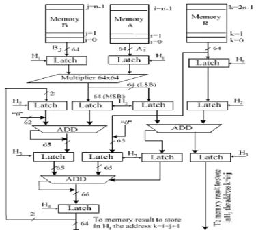
The architecture implementing the method described in the previous section is presented on the figure 5. In this architecture, the operands A and B are first stored in two memories MA and MB of n words of m bits. Each word Ai, Bj of operands A and B is addressed by its weight respectively i and j, which represents their position in the MA and MB memories.
Figure 5. Architecture computing the multi precision multiplication
VIII.
IMPLEMENTATION RESULTS
Our architecture has been implemented using Foundation series 7.1 of Xilinx environment. All modules constituting the architecture have been generated by using the CORE generator system. To guarantee the correct behaviour of our architecture; this last has been simulated using Model Sim PE 6.0, then synthesized employing the XST tool of Xilinx. It has been mapped placed and routed on the Xilinx FPGA circuit of virtex-2 family, the XC2V1000 (-5) bg575.The implementation results of this architecture are presented in the table 1.
IX.
CONCLUSION
REFERENCES
[1]. M.Daumas, F.Dinechin, A, Tisserand, “L’arithmétique des ordinateurs”, <Réseaux et systèmes répartis>- Calculateurs parallèles, Volume 13 n°4-5/2001.
[2]. Douglas N. Arnold, “The Explosion of the Ariane 5”, http://www.ima.umn.edu/~arnold/disasters/ariane.html, 2000. [3]. Douglas N. Arnold, “The Patriot Missile Failure”,
http://www.ima.umn.edu/~arnold/disasters/patriot.html , 2000. [4]. WISE News Communique “Radiological accident in Panama”,
http://www10.antenna.nl/wise/index.html?http://www10.antenna.nl/wise/549 /5278.html, June 2001. [5]. J.-C Bajard. ; L. Imbert; F. Rico, “Evaluation rapide des fonctions élémentaires en multi précision”,
TSI : Technique et Science Informatiques, , Vol. 20, n° 2, pp. 267-286, 2001.
[6]. M.Quercia, “Calcul multi précision”, http://pauillac.inria.fr/~quercia/papers/multiprecision.ps.gz, 2004. [7]. D.M.Smith, “Using Multiple Precision Arithmetic”, Computing in Science &Engineering IEEE