Selective Crossover
as an
Adaptive Strategy for Genetic Algorithms
K anta Prem ji Vekaria
UCL
A dissertation submitted in partial fulfilment of the requirements for the degree of
Doctor of Philosophy
of the
University of London
Department of Computer Science University College London
ProQuest Number: 10011159
All rights reserved
INFORMATION TO ALL USERS
The quality of this reproduction is dependent upon the quality of the copy submitted.
In the unlikely event that the author did not send a complete manuscript and there are missing pages, these will be noted. Also, if material had to be removed,
a note will indicate the deletion.
uest.
ProQuest 10011159
Published by ProQuest LLC(2016). Copyright of the Dissertation is held by the Author.
All rights reserved.
This work is protected against unauthorized copying under Title 17, United States Code. Microform Edition © ProQuest LLC.
ProQuest LLC
789 East Eisenhower Parkway P.O. Box 1346
Abstract
Since the proposal of the first genetic algorithm (GA) many recombination operators have been proposed. Some are problem specific and require a great deal of knowledge about the problem being solved, resulting in good but highly speciahsed operators. Other recombination operators have been proposed for more general use. One advantage for such operators is the httle knowledge required about the problem being solved; however, the synergy of these operators, the problem being solved and other GA parameters does not always yield optimum performance fi-om the GA. More recently, adaptive recombination operators have been proposed to bridge the gap between general and speciahsed recombination operators.
This thesis presents a novel adaptive recombination operator, namely “Selective Crossover”, for use with a genetic algorithm. Selective crossover was designed with three properties that make it a viable strategy to use when Httle or no knowledge is available about the problem being optimised.
The first property is the identification of aUele changes made to the candidate solution during recombination. The second property is the use of correlations between parental and offspring fitnesses to discover beneficial alleles. The third property is the preservation of aUeles at each locus, during recombination, according to their previous contributions to beneficial changes in fitness.
To my brother Lalji, and sisters Bhanu and Damyanti with gratitude and love.
Time passes, There is no way
We can hold it back —
Why, then, do thoughts linger on. Long after everything else is gone?
Acknowledgements
I would like to thank my supervisor Chris Clack for his constant support, encouragement, guidance, constructive criticisms, and for reading multiple drafts of this thesis.
This work was partially funded by EPRSC and the UCL Computer Science Department who never refused me any conference funds. Endless thanks to BBC News Online for allowing me to work on the project at unusual part-time hours, which in turn allowed me to finance my PhD in the first two years. Special thanks to Matthew Karas who made that possible. To Richard Chandler for the many debates about the theory of selective crossover and for answering my endless statistical questions. To Bill Langdon for thoroughly reading and constructively criticising the draft of this thesis. To David Goldberg, Wilham Spears, Lee Altenberg and Richard Watson for their helpful comments and suggestions as well as showing a great deal of enthusiasm and interest in my work. Additional thanks to Wilham Spears for the use of his GA code (GAC) and Mitchell Potter for use of his code on NK landscapes. My gratitude to Kwok Wong for his creative skills in constructing some figures in this thesis.
Contents
1 Introduction...16
1.1 Motivation...17
1.2 Thesis Objective...19
1.3 Contributions... 20
1.4 A Road Map for this Thesis... 21
2 Background Work... 24
2.1 What is a Genetic Algorithm?... 24
2.2 Terminology... 25
2.3 Components of the Genetic Algorithm...26
2.3.1 Population... 26
2.3.2 Evaluation... 28
2.3.3 Selection...29
2.3.4 Recombination...30
2.3.5 Mutation...30
2.4 Choosing Operators and Parameters... 31
2.5 Schema Theorem and Building Block Hypothesis... 33
2.6 Epistasis and Deception...36
2.7 Summary...37
3 Related Work... 38
3.2 Static Recombination Operators...39
3.2.1 One-point Crossover... 39
3.2.2 N-point Crossover...40
3.2.3 Uniform Crossover...40
3.2.4 Bit-Based Simulated Crossover... 41
3.3 Adaptive Recombination Operators... 42
3.3.1 Schaffer and Morishima (1987)... 42
3.3.2 Louis and Rawlins (1991)...43
3.3.3 White and Oppacher (1994)...43
3.3.4 Eshelman and Schaffer (1995)... 44
3.3.5 Spears (1995)...44
3.4 Biases in Static Recombination Operators...45
3.4.1 Positional Bias... 45
3.4.2 Distributional B ias... 45
3.4.3 Exploration and Exploitation...46
3.5 Theoretical Static Recombination Analysis... 47
3.5.1 Framework...47
3.5.2 Schema Survival Probabihty for Uniform Crossover... 47
3.6 Encoding and Linkage in Genetic Algorithms... 49
3.6.1 Holland (1992)...50
3.6.2 Goldberg, Korb and Deb (1989)... 50
3.6.3 Kargupta (1996)... 51
3.6.4 Harik (1997)... 51
3.6.5 Smith (1998)... 51
3.7 Classification of Parameter Adaptation in Genetic Algorithms...52
3.8 Summary... 54
4
Selective Crossover...56
4.1 Inspiration... 56
4.2 Terminology... 58
4.4 Implementation...59
4.5 Mathematical Representation...62
4.6 Review of Properties...65
4.7 Examples of Recombination... 66
4.8 Review of Strategies Used... 70
4.9 Summary and Conclusions... 71
5
Performance Evaluation of Selective Crossover...73
5.1 Experimental M ethod... 73
5.2 GA Parameters... 76
5.3 Test Suite of Benchmark Problems...76
5.3.1 One Max Problem... 77
5.3.2 Royal Road Function... 77
5.3.3 Random L-MaxSAT Problems...79
5.3.4 NK Landscape Problems...81
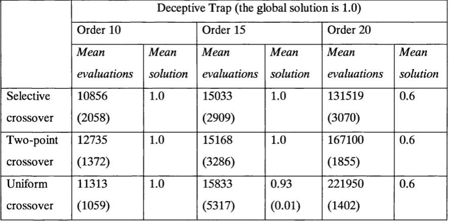
5.3.5 Deceptive Trap Functions... 83
5.4 Experimental Results... 85
5.4.1 One Max Problem...85
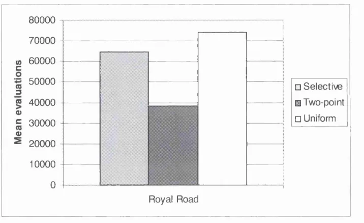
5.4.2 Royal Road Function... 87
5.4.3 Random L-MaxSAT Problems...88
5.4.4 NK Landscape Problems...90
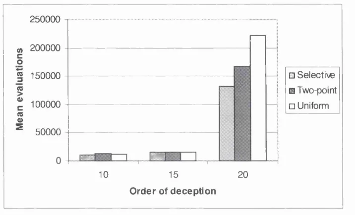
5.4.5 Deceptive Trap Functions...91
5.5 Analysis and Discussion of Results... 93
5.6 Summary and Conclusions...94
6
Features of Adaptation in Selective Crossover... 96
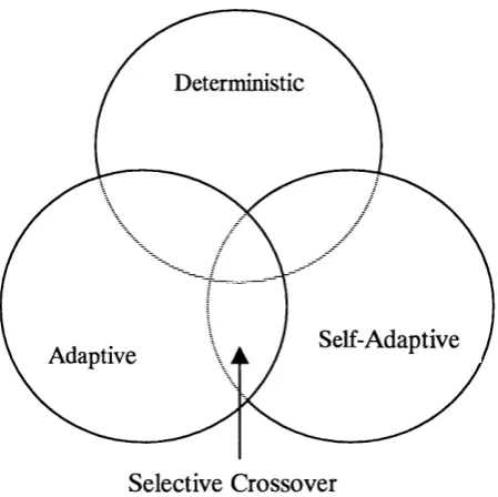
6.1 Classification of Selective Crossover... 96
6.1.1 Deterministic Features...97
6.1.2 Adaptive Features... 98
6.1.4 A New Taxonomy for Type of Change... 99
6.2 Analysis of the Adaptive and Self-Adaptive Features...102
6.2.1 Experiments... 102
6.2.2 Results and Analysis...103
6.3 Analysis of the Dominance Values in the Population...105
6.3.1 Experiments...105
6.3.2 Results and Analysis...106
6.4 Summary and Conclusions...110
7 Biases in Adaptive Recombination Operators... 112
7.1 Existing AUele-Based Adaptive Recombination Operators... 113
7.1.1 Masked Crossover... 113
7.1.2 Adaptive Uniform Crossover...116
7.2 Analysis of Biases in Allele-Based Adaptive Recombination Operators...119
7.2.1 Directional Bias...119
7.2.2 Credit Bias...119
7.2.3 Initiahsation B ias...120
7.2.4 Hitchhiker Bias...122
7.2.5 Interdependencies Between Biases... 123
7.3 More Hitchhiking and Selective Crossover... 125
7.4 Analysis of the Effect of Biases on Selective Crossover... 127
7.4.1 Selective Crossover with Less Credit Bias...129
7.4.2 Selective Crossover without the Initiahsation Bias... 131
7.4.3 Results... 132
7.5 Analysis... 134
7.6 Summary and Conclusions...136
8
Schema Propagation in Selective Crossover...138
8.1 Alternative Royal Road Encodings... 139
8.2 Analysis of Schema Propagation...142
8.2.2 Results on Performance...144
8.2.3 Results on Schema Propagation...145
8.2.4 Analysis... 147
8.3 Schema Survival Probability for Selective Crossover... 151
8.4 Summary and Conclusions...157
9
Conclusions... 160
9.1 Discussion of Results... 160
9.2 Contributions of this Thesis...163
9.3 Limitations of this Thesis... 164
9.4 Future Work...165
Bibliography...168
List of Figures
Figure 2.1: Generational cycle of a conventional genetic algorithm... 27
Figure 3.1: One-point crossover... 40
Figure 3.2: Two-point crossover... 40
Figure 3.3: Uniform crossover... 41
Figure 3.4: An example of hyperplane survival - Parent 1 is a member of the third-order hyperplane H3 = “* * m ” and Parent2 is an arbitrary string. Recombination is performed to produce two offspring... 48
Figure 4.1: A Generational Cycle of a Genetic Algorithm using Selective Crossover 59 Figure 4.2: An individual in selective crossover consists of an additional dominance vector...60
Figure 4.3: Recombination with Selective Crossover... 61
Figure 4.4: Updating Dominance Values...61
Figure 5.1: Simple Royal Road Function...79
Figure 5.2: An example of epistatic interactions for an NK landscape where N=4 and K=2... 82
Figure 5.3: A Deceptive Trap function where a bit string of aU Is is the global optimum and a bit string of all Os is the local optimum... 84
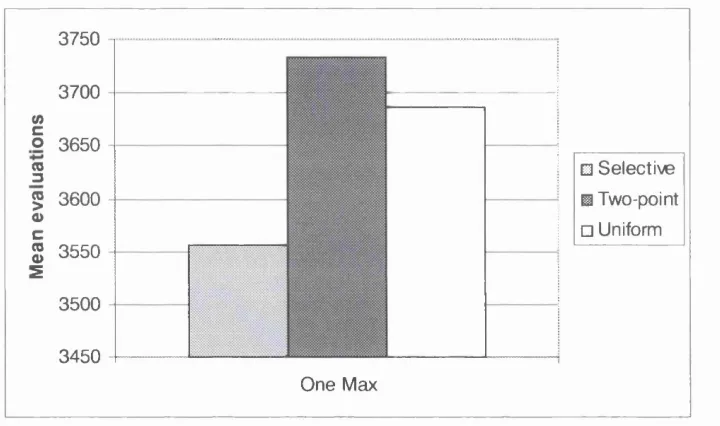
Figure 5.4: Results for the One Max problem - performance comparison of selective, two-point and uniform crossover... 86
Figure 5.5: Results for the Royal Road function - performance comparison of selective, two-point and uniform crossover... 87
selective, two-point and uniform crossover... 90 Figure 5.8: Results for the Deceptive Trap problems - performance comparison of
selective, two-point and uniform crossover... 92 Figure 6.1: Taxonomy of parameter control by Eiben et al. (1999)...97 Figure 6.2: New taxonomy for type of parameter control... 100 Figure 6.3: Classification of other adaptive recombination operators using this new
taxonomy... 101 Figure 6.4: GA Cycle of selective crossover that does not change the dominance
values... 103 Figure 6.5: The evolution of the distribution of dominance values in the population, for
the One Max problem... 107 Figure 6.6: The evolution of the distribution of dominance values in the population, for
the Royal Road function...108 Figure 6.7: The evolution of the distribution of dominance values in the population, for
the NK Landscape N=32 K=8... 109 Figure 7.1: Recombination using masked crossover...114 Figure 7.2: Masked crossover - creation of new binary masks if both children are
‘good’. (? Denotes randomly generated)... 114 Figure 7.3: Masked crossover - creation of new binary masks if both children are
‘bad’. Assume fitness of Parent2 > Parent 1. (? Denotes randomly generated) 114 Figure 7.4: Recombination using adaptive uniform crossover (AUX). The automata
belonging to the offspring are updated here given that the fitness of Child 1 > Parent 1, Parent2 and fitness of Child2 < Parent 1, Parent2...117 Figure 7.5: Population of 4 individuals, which demonstrates that the dominance values
are not uniformly distributed at each locus due to the small population size. As the population size increases the distribution of the dominance values at each locus is more likely to be uniform... 121 Figure 7.6: Example of hitchhiker bias in selective crossover when apphed to the One
Max problem... 123 Figure 7.7: Interdependencies amongst biases in allele-based adaptive recombination
operators...124 Figure 7.8: Reducing the magnitude of the credit bias by sharing the fitness increase
Since two alleles were exchanged their dominance values get increased by 0.05 (0.1/2)... 130 Figure 7.9: Selective crossover without the initiahsation bias... 131 Figure 8.1: Encoding A -the original encoding of a Royal Road function. In this
encoding the defining length of level 0 schemata, ô(level 0), is 7... 140 Figure 8.2: Encoding B - A new encoding of a Royal Road fimction. In this encoding
the defining length of level 0 schemata, ô(level 0), is 14... 141 Figure 8.3: Encoding C - A new encoding of a Royal Road function. In this encoding
the defining length of level 0 schemata, 0(level 0), is 28... 141 Figure 8.4: Encoding D - A new encoding of a Royal Road function. In this encoding
the defining length of level 0 schemata, ô(level 0), is 56... 142 Figure 8.5: Example of schema propagation in a single recombination event. Parent 1
contains schemata SI, S3 and S7. Parent2 contains schemata SI, S4, S8. Schemata SI and S3 were propagated fi"om Parent 1 and schemata SI, S4 and S5 were propagated from Parent2... 143 Figure 8.6: Schema propagation in two-point crossover with different Royal Road
encodings. DL# is the defining length of level 0 schemata. The results show the number of level 0 schemata propagated per individual at each generation...146 Figure 8.7: Schema propagation in uniform crossover with different Royal Road
encodings. DL# is the defining length of level 0 schemata. The results show the number of level 0 schemata propagated per individual at each generation...146 Figure 8.8: Schema propagation in selective crossover with different Royal Road
encodings. DL# is the defining length of level 0 schemata. The results show the number of level 0 schemata propagated per individual at each generation...147 Figure 8.9: Encoding A - the original Royal Road encoding where the defining length
of level-0 schemata ô(level-O) =7. A comparison of schema propagation between two-point, uniform and selective crossover... 148 Figure 8.10: Encoding B - a Royal Road encoding where the defining length of level-0
schemata ô(level-O) =14. A comparison of schema propagation between two-point, uniform and selective crossover...149 Figure 8.11: Encoding C - a Royal Road encoding where the defining length of level-0
two-point, uniform and selective crossover... 149 Figure 8.12: Encoding D - a Royal Road encoding where the defining length of level-0
List of Tables
Table 2.1: An example collection of operators and parameters associated with a genetic algorithm...31 Table 5.1: A table of fitness contributions for the NK landscape given in Figure 5.2...82 Table 5.2: Results for the One Max problem. Mean number of evaluations taken to
solve the One Max problem. The standard deviation is shown in brackets... 86 Table 5.3: Results for the Royal Road function. Mean number of evaluations taken to
solve the Royal Road function. The standard deviation is shown in brackets... 87 Table 5.4: Results for the Random L-MaxSAT problems. Mean number of evaluations
to find the best solution for low, medium and high epistasis. The standard deviation is shown in brackets... 88 Table 5.5: Results for the NK Landscape problems. Mean number of evaluations to
find the best solution for K=4, 20 and 31. The standard deviation is shown in brackets...90 Table 5.6: Results for the Deceptive Trap problems. Mean number of evaluations
completed for order 10, 15 and 20 partially deceptive trap functions. The standard deviation is shown in brackets. The solution quality is given in square brackets 91 Table 5.7: A summary of relative performance of selective, two-point and uniform
crossover. A 1* represents best performance... 93 Table 6.1: Results of applying selective crossover without its adaptive feature to the
One Max, Royal Road and NK landscapes. Previous results with adaptive feature are also recalled in this table...104 Table 7.1: Updating rules for adaptive uniform crossover (AUX). +?superiorReward is the
to the previous state... 116 Table 7.2: Relative strength of biases present in masked crossover, adaptive uniform
crossover and selective crossover... 124 Table 7.3: Mean fitness of best solution found when analysing the biases in selective
crossover without mutation in the GA. Results are from 50 independent runs for the Royal Road and NK Landscape problems. The standard deviation is shown in brackets... 132 Table 7.4: Mean solution found and mean evaluations taken when analysing the biases
in selective crossover with mutation in the GA. These are results from 50 independent runs for the Royal Road function. On all runs the global solution was found. The standard deviation is shown in parentheses... 133 Table 7.5: Mean solution found and mean evaluations taken when analysing the biases
in selective crossover with mutation in the GA. Results from 50 independent runs for NK landscapes N=32 K= {4,20,31}. The standard deviation is shown in parentheses...133 Table 8.1: Mean number of evaluations taken to find the solution for different Royal
Chapter 1
Introduction
The fundamental problem of optimisation is to arrive at the best possible decision in any given set of circumstances. There are many situations where the ‘best’ is unattainable for one reason or another; often we may not be sure what is meant by the ‘best’. The first step therefore in an optimisation problem is to choose some quantity, typically a function of several variables, to be maximised or minimised, subject possibly to one or more constraints. The commonest types of constraint are equahties and inequalities, which must be satisfied by the variables of the problem. The next step is to choose a method to solve the optimisation problem; such methods are usually called optimisation techniques, or optimisation algorithms. One such algorithm is the genetic algorithm.
First pioneered by John Holland in the 1960s (Holland 1992), genetic algorithms have been demonstrated to be a successful optimisation algorithm. They were inspired by, and mimic, some of the processes observed in natural evolution. Based on the Darwinian principle of ‘survival of the fittest’, genetic algorithms manipulate a population of candidate solutions using selection, recombination and mutation processes. These processes allow good solutions to survive in preference of weaker ones.
The genetic algorithms that have been proposed for optimisation problems in recent years have tended to become more and more elaborate (Goldberg 1989a; Michalewicz 1994, Back 1996; Mitchell 1996); the result being a large parameter space for a genetic algorithm. Thus, choosing the appropriate parameters for a genetic algorithm has become a more difficult task and is in itself an optimisation problem.
of genetic algorithms and is thought to be responsible for the generation and propagation of solutions (Holland, 1992; Schaffer and Eshelman, 1991; Spears, 1993). Since the proposal of the first genetic algorithm many recombination operators have been developed. Some are problem specific and require a great deal of knowledge about the problem being solved, resulting in good but highly speciahsed operators. For example, on ordering problems a number of recombination operators have been proposed that respect the ordering of alleles (Goldberg and Lingle, 1985; Starkweather et al., 1991; Falkenauer, 1994). Other recombination operators have been proposed for more general use (De Jong, 1975; Syswerda, 1989; Spears and De Jong, 1991b). One advantage for general operators is the httle knowledge required about the problem being solved; however, the synergy of these operators and the problem being solved and other parameters does not always yield best performance from the genetic algorithm. More recently, adaptive recombination operators have been proposed to bridge the gap between general and speciahsed recombination operators (Schaffer and Morishima, 1987; Louis and Rawhns, 1991; White and Oppacher, 1994; Eshelman and Schaffer, 1995; Spears, 1995). The aim of these adaptive methods is to adapt dynamicaUy to problem characteristics in the hope of creating a more robust optimisation strategy. We know from “No Free Lunch” theorems (Wolpert, and Macready 1997) that an algorithm that is suited for ah problems cannot exist, since for fixed parameter/operator sets there wih be problems for which they are optimal and other problems for which their performance is poor. However, is it possible to devise an adaptive recombination operator that is a suitable strategy to use for a wide range of problems in which httle is known about the problem space being searched?
1.1 Motivation
genes and a subset of these genes last for many more generations because it is the genes that are passed onto the offspring not the entire chromosome. Thus natural selection favours the gene.
Dominance in nature is associated with genetic material within diploid chromosomes (two sets of chromosomes) where the alleles contained in one set can be regarded as a direct alternative to the alleles in the other set. When building the organism the alleles in one set compete with those in the other set. Alleles that are dominant are expressed in the phenotype of an organism and those that are less likely to be expressed are recessive. The relationship between a dominant and recessive gene is complex: some genes that have been known to be dominant have become more recessive in successive generations and vice versa. Merrell (1984) suggests that these shifts in dominance are in response to changes in the environment. Thus, those genes that increased an individual’s fitness have become more dominant by evolving over generations; however, a precise model to show this is not available.
Selective crossover, our new adaptive recombination operator, uses both the analogy of dominance, where alleles in one chromosome compete with those on the other chromosome, and the analogy of evolution of dominance. The purpose is to see if recombination at each allele in a haploid (single chromosome) genetic algorithm can be evolved such that alleles in one parent compete with those on the other parent chosen for crossover. Here the alleles are competing to be retained in a fitter individual and the use of correlations between parental and offspring fitnesses would allow the means of discovering beneficial alleles. This in turn allows recombination in the genetic algorithm to adapt to the problem space being searched.
1.2 Thesis Objective
This thesis examines the following hypothesis:
Hypothesis:
When little or no knowledge is available about the problem being optimised by a genetic algorithm, a viable strategy is to use an adaptive recombination operator with the following three properties:
1. Detection - It detects alleles that were changed during recombination to identify modifications made to the candidate solution.
2. Correlation - It uses correlations between parental and offspring fitnesses as a means o f discovering beneficial alleles.
3. Preservation - It preferentially preserves alleles at each locus, during recombination, according to their previous contributions to beneficial changes in fitness.
There are two main aims of this thesis. First, to design and implement a new adaptive recombination operator, “selective crossover'' with the above three properties. Second, to undertake an extensive evaluation of selective crossover using four different criteria. As we shall see, both aims have been achieved.
Selective crossover was designed with three key properties. Firstly, selective crossover detects alleles that were changed during crossover to identify actual modifications made to the candidate solution during recombination. Secondly, this acquired knowledge is then combined with parental and offspring fitness correlations to discover potentially beneficial alleles. Finally, alleles are preferentially preserved, during recombination, according to their previous beneficial fitness contributions.
operators, two-point and uniform crossover, on a set of five different and well-studied benchmark problems. Given our performance measure selective crossover was demonstrated to be better or comparable to two-point and uniform crossover on most problems.
The second evaluation in terms of adaptive features within selective crossover allowed us to observe empirically the dynamics of selective crossover on different problems. This confirmed the internal adaptive behaviour of selective crossover and also demonstrated that selective crossover adapts to each problem in a different manner.
The third evaluation was completed by a critical analysis of the biases that selective crossover imposes on search. This identified some limitations and possible enhancements to selective crossover.
The final evaluation, in terms of schema propagation, was undertaken using different encodings of a problem and tracking schema, in the population, before and after recombination. The alternative encodings positioned genes at different locations on the chromosome and were used to analyse the affect they have on the performance of selective crossover, two-point crossover and uniform crossover. The schema propagation of all three recombination operators was compared, allowing three conclusions to be drawn. Firstly, the performance of selective crossover is consistent regardless of the encoding used. Secondly, the survival rate of a schema in selective crossover is not affected by the encoding. Thirdly, selective crossover provides a better balance between exploration and exploitation than the two other traditional recombination operators.
1.3 Contributions
This thesis makes six main contributions.
1. The design and implementation of “selective crossover”, a new adaptive recombination operator that incorporates correlations between parents and offspring as a means of discovering and preserving beneficial alleles at each locus during recombination to produce fitter offspring.
3. An empirical analysis that demonstrates adaptive behaviour in selective crossover.
4. An identification of four key biases inherent in selective crossover, a demonstration of the existence of these biases in two other similar operators and an empirical analysis to study the effects of these biases on selective crossover.
5. An analysis and comparison of schema propagation in selective crossover and two traditional recombination operators.
6. A construction of a schema survival probabihty for selective crossover; this demonstrates that schema survival in selective crossover is problem dependent.
This thesis also makes a secondary contribution; a description of a new taxonomy to classify selective crossover and other adaptive strategies in evolutionary computation, which overcomes the limitations in the existing taxonomy provided by Eiben et al.
(1999)(described in Chapter 3).
1.4 A Road Map for this Thesis
After this introduction Chapter 2 presents a traditional genetic algorithm. It highhghts both the vast parameter space associated with genetic algorithms and the issues surrounding the choice of parameters that have led to the development of adaptive strategies. Additionally, Chapter 2 presents the original theoretical explanation of genetic algorithms, due to Holland (1992) and discusses the concepts of epistasis and deception.
Chapter 3 focuses on the recombination operator and provides a survey of work on static recombination operators, adaptive recombination operators and strategies proposed to learn linkage. It also presents theoretical work on schema survival in static recombination operators. The increase in adaptive strategies has led to many classifications of adaptation that are also presented here.
Chapter 5 provides an empirical evaluation in terms of performance. Selective crossover is compared with two static recombination operators, two-point and uniform crossover (described in Chapter 3), on a set of five different and well-studied benchmark problems. This evaluation shows that the performance of selective crossover is either superior or comparable to two-point and uniform crossover.
Chapter 6 identifies the limitations of the taxonomy to classify adaptive strategies provided by Eiben et a l (described in Chapter 3). A new taxonomy is presented which accommodates strategies that use one or more methods of change. This new taxonomy is also used to classify and identify the methods of change in selective crossover. An empirical analysis demonstrates that without the three key properties (see hypothesis), the performance of selective crossover is worse than two-point and uniform crossover. This chapter also provides an empirical analysis of the adaptive behaviour in selective crossover. The experiments to track the population dynamics conclude by demonstrating that selective crossover adapts recombination and also suggests that selective crossover adapts to the problems being optimised, in contrast to static behaviour.
Chapter 7 presents a critical analysis of selective crossover and two other similar adaptive recombination operators. Four key biases were identified to be inherent in selective crossover; directional, credit, hitchhiker and initialisation bias. Experiments show that some of these biases are detrimental to the performance of selective crossover; however they can be reduced and thus further enhance selective crossover.
Chapter 8 describes a series of experiments to investigate schema propagation in selective crossover. Two conclusions result from these experiments: firstly, selective crossover is insensitive to the encoding of gene positions in the chromosome, unlike other recombination operators. Selective crossover shows consistent behaviour even when the encoding is altered so that related genes are located at the extremes of the chromosome. Secondly, when the schema propagation of selective crossover is observed and compared with two-point and uniform crossover, selective crossover appears to provide more exploration in early generations and more exploitation in later generations in comparison to the other two operators.
Chapter 2
Background Work
The aim of this chapter is to set the scene for this thesis by providing an introduction to the conventional genetic algorithm. We first provide (in Section 2.1) an introductory paragraph to set genetic algorithms in context with other evolutionary algorithms. This is followed by an introduction to the terminology drawn from natural genetics that is used in genetic algorithms. Section 2.3 then provides a description of each component in a conventional genetic algorithm and Section 2.4 highlights the many operators and parameters associated to the genetic algorithm and how difficult it is to choose appropriate settings that give best performance. A brief explanation of the schema theorem and building block hypothesis is provided in Section 2.5. Finally, Section 2.6 introduces two concepts, epistasis and deception, which are used in GA research to characterise problems in terms of difficulty and are used in this thesis to choose problems that serve as a good test-bed to evaluate selective crossover.
2.1 What is a Genetic Algorithm?
Genetic Programming (Koza 1992), However, G As have four elements that together differentiate them from these other evolutionary algorithms:
1. A population of chromosomes. 2. Selection according to fitness.
3. Recombination to produce new offspring. 4. Random mutation of new offspring.
Many of the terms used in G As are drawn from biology hence we first introduce the terminology in the next section.
2.2 Terminology
All hving organisms consist of ceUs, and each cell contains the same set of one or more
chromosomes. A chromosome is comprised of numerous genes that encode for a particular trait, such as eye colour. The set of possible values taken up by each trait are called alleles (e.g. blue, green, brown). The position of a gene is defined by its locus and is identified separately from the gene’s function.
Many organisms have multiple chromosomes in each cell. Those organisms with a pair of chromosomes are called diploid and organisms with a single set of chromosomes are called haploid. In nature, most sexually reproducing organisms are diploid.
Sexual reproduction in diploid and haploid organisms occurs in different ways. During diploid sexual reproduction, recombination (or crossover) takes place. In each parent a gamete (new single chromosome) is formed by combining genes between each pair of chromosomes. The gametes from the two parents combine to create a complete set of diploid chromosomes. In haploid sexual reproduction, genes are exchanged between two parents’ single-strand chromosomes to form the new haploid chromosome. Mutation
takes place due to recombining errors and is usually an allele change in offspring. The
fitness of an organism is defined as the probabihty that the organism will survive to reproduce.
Most GA appHcations use haploid (single-chromosome) individuals. The term
called loci. Each gene encodes to a particular element, trait, of the candidate solution. The values taken up by a gene are alleles and are defined by the alphabet used to make up the candidate solution. Given a bit string representation the alphabet is the set {0,1} and thus an allele is either 0 or 1. The set of parameters presented by a particular chromosome is referred to as a genotype. The genotype contains the information to construct the solution (as in genetic terms to construct the organism), which is referred to as the phenotype.
2.3 Components of the Genetic Algorithm
In this section we describe a conventional genetic algorithm (GA), which is just one of the many ways of implementing a GA. For an extensive review of current strategies and alternative implementations of the GA the reader is referred to Goldberg (1989a), Michalewicz (1994) and Mitchell (1996).
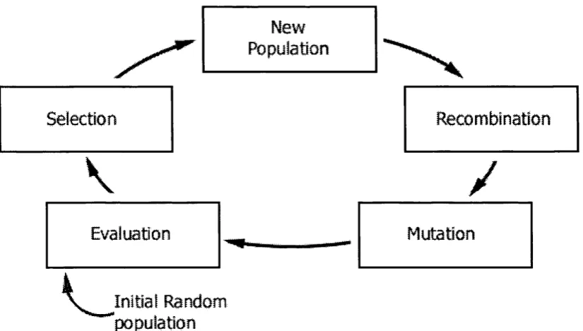
The conventional GA is comprised of five components: population, evaluation, selection, recombination and mutation. The use and issues surrounding each component are highhghted in the successive sub-sections. Each cycle of a GA is called a generation
and is represented as shown in Figure 2.1 and Algorithm 2.1. In each generation the GA manipulates a population of chromosomes or individuals using evaluation, selection, recombination and mutation processes. The GA continues to run through many generations until either a solution is found or once a fixed number of generations have elapsed; this termination criterion is pre-determined by the GA practitioner.
2.3.1 Population
The GA maintains a population of chromosomes, candidate solutions, with associated fitness values. Therefore, before a GA can be run a suitable encoding or representation of the problem must be estabhshed. An encoding consists of a string of parameters related to the problem. For example, consider a parameter optimisation problem where a set of variables need to be optimised; to minimise or maximise some function F(xi, X 2 , . . . . , X n ) .
Population
Evaluation Mutation
population
Figure 2.1: Generational cycle of a conventional genetic algorithm.
Procedure Genetic_Algorithm;
T=0; /* starting generation */ Initialise_population(P); E v a l u a t i o n ( P ) ;
WHILE NOT finished DO {
T=T+1; /* Next generation */ Se lection(P);
R e c o m b i n a t i o n (P ); M u t a t i o n (P ); Eval u a t i o n ( P ) ;
}
Algorithm 2.1: Pseudo code for a conventional genetic algorithm.
suggested that there are more theoretical advantages in using a binary encoding. However, Antonisse (1989) and Radcliffe (1992) have questioned these arguments. Additionally, empirical comparisons between binary encodings and multiple character encodings have shown better performance for the latter Michalewicz (1994). At present there are no conclusive findings that suggest the use of a particular encoding.
Other issues related to the encoding is the loci at which genes should be placed on the chromosome. Goldberg (1989a) suggests that genes should be strategically placed on the chromosome so that their positions can be exploited by the recombination operator. This is further discussed in the next chapter (Section 3.4).
Having estabhshed the encoding for the problem a population of candidate solutions must be created and the question is how many (the population size)? In most G As a fixed sized population is used and is a fundamental decision faced by GA practitioners. If too smaU a population size is chosen, the GA wih converge too quickly with insufficient processing of possible solutions. On the other hand, a population with too many members consumes a great deal of processing power with very httle payoff in terms of better solutions. Several researchers have investigated the size of the population using binary encodings. Goldberg (1989b) suggests that the optimal population size grows exponentiaUy with the length of the chromosome, which in a practical sense are extremely large populations. Grefenstette (1986) suggests the use of a small population size of 30 individuals. More recently. Reeves (1993) provides a theoretical justification for the use of smaller population sizes. Most usually optimum population sizes are constrained by the available machine resources and thus a strong preference is for small populations.
Having decided the population size p, the starting population is initiahsed by randomly generating p chromosomes. For the GA cycle to begin the chromosomes must first be evaluated and this is discussed in the next section.
2.3.2 Evaluation
proportionate to the performance of the phenotype. The fitness function is usually given as part of the problem; in our previous example on function optimisation the fitness function is just the value returned by the function. However, it is not always so straightforward.
2.3.3 Selection
GA search is directed by selection with a bias towards areas in the search space that contain better solutions. The purpose of selection is to choose candidate parents for the process of recombination such that prominence is given to fitter individuals. There are many strategies to use for selection. Strong selection can lead to premature convergence, where a large proportion of the population consists of identical chromosomes that represent sub-optimal solutions. Weak selection on the other hand can make the search ineffective, where search makes very httle progress in comparison to the resources being used. Numerous selection schemes have been proposed and compared in GA hterature (Goldberg and Deb 1991; Thierens and Goldberg 1994; BHckle and Thiele 1995; Back
1996). A description of the most popular methods is given below.
2.3.3.1 Fitness Proportionate Selection
In fitness proportionate selection the expected number of offspring of an individual is equal to the fitness of that individual divided by the average fitness of the population. The most common method to implement this is the ‘roulette wheel’: each individual in the population is assigned a slot sized in proportion to its fitness. The wheel is spun N times (where N is the population size). The individual pointed by the wheel marker is selected.
Given a large enough population, this roulette wheel selection method will theoretically result in the expected number of offspring for each individual. However, the actual number of offspring allocated is far from the expected values. Baker (1987) proposed a different sampling method namely ‘stochastic universal sampling’ (SUS). This algorithm is analogous to roulette wheel but in this case the wheel is not spun N times but once using N equally spaced pointers. The number of copies an individual receives is then given by the number of pointers that fall in its slot.
2.3.3.2 Tournament selection
Tournament selection chooses some number t (tournament size) of individuals randomly from the population and copies the best individual from this group into the intermediate population. This is repeated N times to make up the N individuals in the population. In most cases the tournament size is two, but larger tournament sizes can be used in order to increase the selection pressure.
2.3.3.3 Ranking Selection
Baker (1985) introduced ranking selection as a way of relaxing the selection pressure to prevent premature convergence. The population is first sorted from best to worst. The expected value of offspring for each individual is a function of its rank. This selection method avoids giving the largest share of offspring to a small group of highly fit individuals and thus reduces the selection pressure.
2.3.3A Elitism
Ehtism or an ehtist strategy, first introduced by De Jong (1975), is a form of selection that is used together with the other selection methods like those described above. This strategy ensures that highly fit individuals in the population are passed onto the next generation without being altered by the recombination or mutation operators. This guarantees that the maximum fitness of the population can never reduce from one generation to the next.
2.3.4 Recombination
Recombination or crossover takes two individuals, and combines their chromosomes to create two offspring. Associated with recombination is the crossover rate - the probabihty that any individual will experience crossover, and unless it is set to 1, there is a chance some members in the current generation do not undergo crossover. The three most popular types of crossover are one-point crossover, two-point crossover and uniform crossover; these are further discussed in Section 3.2.
2.3.5 M utation
fixation on the search space. For example, without mutation, every string in the population may hold a one at the first bit position, and there would be no way of obtaining a zero at the first position. Therefore mutation is what helps provide diversity at a given bit position.
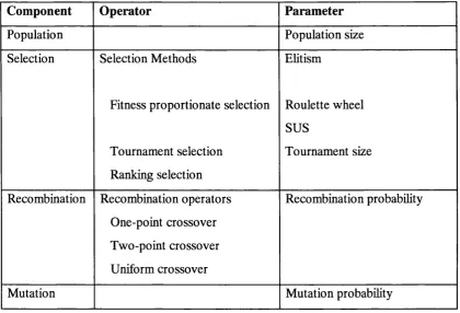
2.4 Choosing Operators and Parameters
In Section 2.3, a description of the components was provided and all but one component (evaluation) has associated with it a choice of operators and/or parameters. An example of possible choices that can be made is given in Table 2.1. There are many more GA operators and parameters; a comprehensive survey can be found in Michalewicz (1994) and Mitchell (1996).
Component O perator Param eter
Population Population size
Selection Selection Methods
Fitness proportionate selection
Tournament selection Ranking selection
Ehtism
Roulette wheel SUS
Tournament size
Recombination Recombination operators One-point crossover Two-point crossover Uniform crossover
Recombination probabihty
Mutation Mutation probabihty
Table 2.1: An example collection of operators and parameters associated with a genetic algorithm.
Earlier work has been done on trying to find suitable choices of operators and parameters that will work well on a wide range of problems. De Jong (1975) put considerable effort into finding ideal parameter values, for a traditional GA, that were good for a suite of test problems also proposed in his work. He used an experimental approach and concluded that the following parameters gave reasonable performance:
Population size 50 - 100
One-point crossover rate 0.6 Mutation probability 0.001
Selection strategy ehtist + roulette wheel
In a further study, Grefenstette (1986) used a ‘meta-GA’ to optimise values for the parameters. He also used De Jong’s test suite and evolved a population of 50 GA parameter sets (the same set used by De Jong). His study found parameters:
Population size 30
One-point crossover rate 0.95 Mutation probabihty 0.01
Selection strategy ehtist + roulette wheel
Note how the parameter settings differ in both studies. An exhaustive study by Schaffer et al. (1989) on a smah set of numerical optimisation problems and on some functions from De Jong’s test suite also arrived at different conclusions.
differ over the course of a single run as was demonstrated by approaches that adapt recombination and mutation probabilities concurrently with ongoing search (Davis 1989; Back 1992a and 1992b; Tuson and Ross 1998). Other adaptive techniques such as adaptive recombination operators have been proposed and are further discussed in Section 3.3.
2.5
Schema Theorem and Building Block Hypothesis
The first theoretical foundation of genetic algorithms was presented by Holland (1992); this is known as the Schema Theorem and assumes a binary encoding of chromosomes. Holland (1992) introduced the concepts of schemata and building blocks, which have now dominated much of the theoretical analysis and thinking about G As.
A schema is built by introducing a "don’t care’ symbol (*) into the alphabet of genes. For example, in a binary encoding a schema is a string of characters from the alphabet {0, 1, *}. A schema represents all strings, or “hyperplanes” (subsets of the search space), which match it on all positions other than For example, a schema H I = “*0000” is a hyperplane defined by having zeros in its last four positions. All strings with zeros in their last four positions are examples or instances of this schema. Thus schema HI matches 2 strings and for example:
H2 = “1*1*0” matches 4 strings H3 = “0***0” matches 8 strings H4 = “***1*” matches 16 strings
H5 = “*****” matches 32 Q! where I is the length of the string) strings
There are two properties used to describe schemata, the order and defining length. The Schema Theorem is formulated using these two properties and this terminology is also used throughout this thesis. The order of a schema H, denoted by o(H) is the number of non-* symbols in the schema. For example, the following 3 schemata, each of length 5,
have the following orders:
o(H l) = 2, o(H2) = 3 and o(H3) = 5.
The defining length of a schema H, denoted by ^ H ), is the distance between the first and last non-* symbol. For example,
Ô (HI) = 1 ,0 (H2) = 3 and (5 (H3) = 4.
Holland (1992) showed that the analysis of GA behaviour was far simpler if carried out in terms of schemata. He showed that a string of length I is an instance of 2^ schemata. In theory a population of P individuals could contain P 2^ schemata but in general not aU schemata will be represented, as there will be some overlap. Holland was able to demonstrate, using the Ar-armed bandit analogy, the result known as “implicit parallelism". This suggests that the main factor in the success of G As is their ability to
test a large number of possibilities such that a population will usefully process O(P^) schemata. However the vahdity of this argument has attracted many criticisms. Firstly the notion of imphcit parallehsm assumes a uniformly distributed population and in a GA that is true only in the initial population. Grefenstette (1991) states that in order to accurately assess how many hyperplanes are processed it is necessary to consider the dynamic distribution of samples within the population which means taking into account the fitness function and selection algorithm as part of the analysis. Secondly, the assumption that hyperplane competitions can be isolated and solved independently is incorrect owing to high fitness variances (Grefenstette and Baker 1989) and gene interactions (Reeves and Wright 1999). Thus, the fitness of a hyperplane cannot be estimated independently of those with which it interacts. Macready and Wolpert (1996) have also argued, using the 2-armed bandit analogy, that the strategy described by Holland is not an optimal one. Furthermore they also believe there is a fatal flaw in Holland’s analysis and its supposed justification for G As.
Schema Theorem provides a lower bound on the expected number of instances of schema
H at time t + 1, denoted as E\m {H ,t + l)\, as being a function of the number of instances
of schema H at time t (denoted as w(H, t)), the probability of selecting schema H, and the probabihty of disrupting H via recombination and mutation (as given below):
E\m{H ,t +1)] ^ m(H, t) * probabihty of selection * (1 - probabihty of disruption)
The Schema Theorem provides a lower bound because recombination and mutation may
also create instances of a schema H. E\m {H ,t +1)] is given as:
Where:
f ( H , t ) represents the mean fitness of individuals that are instances of schema H
at time t,
f ( t ) represents the mean fitness of the population at time t,
is the recombination rate,
is the mutation rate.
The Building Block Hypothesis (Goldberg 1989a) is related to the Schema Theorem. This states that G As work by discovering low-order schemata of high fitness {building blocks)
and then combining them via recombination to form higher-order fitter schemata. However this still remains unproven and is an article of faith, which for some problems is easily violated. Consider the following a problem that has a global optimum (the fittest individual in the search space) HG = “11111” and a local optimum (a false peak) HL = “00000”. Now consider the following schemata that have above average fitness:
The combining of these schemata produces a schema H3 = which might be less fit than H I and H2 and furthermore might be less fit than schemata:
H4 = “00***” H5 = “***00” H6 = “00*00”
In these cases the GA may have difficulty in converging to HG since it may tend to converge to strings leading to HL. This phenomenon is called deception and is described in more detail in the next section.
2.6 £pistasis and Deception
A central problem in the theory of G As is the characterisation of problems that are difficult for G As to optimise. Many attempts to characterise such problems have focused on the notion of epistasis and deception.
Epistasis is the interaction of genes in a chromosome. That is, the influence of a gene on the fitness of the chromosome may depend on the values (alleles) of other genes present on the chromosome. This interaction does not just apply to genes that are grouped together on the chromosome. Interaction can occur between genes at opposite ends of the chromosome or between adjacent genes. Moreover each gene can have different interactions with each other; some genes may not interact with others on the chromosome whilst some may interact with many. Most problems contain epistasis; however, it is difficult to know a priori exactly how much epistasis exists in a problem.
single schema that is not the global optimum. A partially deceptive problem of order k
exists when the maximum order of any schema is greater than k and all relevant hyperplanes of order less than k lead toward a single schema that is not the global optimum.
In our test-suite of benchmark problems (Section 5.3) we use L-MaxSAT problems (Mitchell, Sehnan and Levesque 1992; De Jong, Potter and Spears 1997) and NK landscapes (Kauf&nan, 1993) with tuneable epistasis and deceptive trap functions (Deb and Goldberg 1993) with tuneable deception which allows us to evaluate performance of recombination operators under a wide range of conditions.
2.7 Summary
The genetic algorithm is a type of evolutionary algorithm that uses a genetic/evolutionary metaphor. Implementations typically use fixed-length bit chromosomes to represent the genetic information, together with a population of individuals that undergo recombination and mutation in order to find optimal solutions.
The conventional GA has many components each associated with operators and parameters. The number of parameters available to use today are far greater than that of the original GA proposed by Holland (1992) and as the search capabilities of the GA are sensitive to the combination of the parameters chosen, the choice of parameters to use is difficult to decide a priori.
Chapter 3
Related Work
This chapter is focussed on recombination and begins with a survey of previous work on recombination operators by dividing these operators into two sets: static and adaptive.
3.1 Introduction to Recombination
Recombination, also known as crossover, has been considered as the primary operator of a GA (Holland 1992; Goldberg 1989a) and is thought to be responsible for the generation and propagation of good solutions. More recently, there have been many studies on the role played by traditional static recombination operators compared with the role of mutation in a GA (Schaffer and Eshelman 1991, Spears 1993 and Wu, Lindsay and Riolo 1997). Recombination operators have also been classified by their usefiilness in terms of generating and propagating solutions (Eshelman and Schaffer 1995). There are now many different ways of implementing recombination (Spears 1997). Some recombination operators incorporate adaptive methods and are classed as adaptive recombination operators: those that do not incorporate adaptive methods are classed as static recombination operators.
3.2 Static Recombination Operators
In this section we describe static recombination operators that have been considered for use as general operators. The three most popular recombination operators are one-point, two-point and uniform crossover. The popularity of one-point crossover is due to the foundations of genetic algorithms constructed by Holland (1992). Two-point crossover (De Jong 1975) and uniform crossover (Syswerda 1989) are also popular, as they have been shown to perform better than one-point crossover (Syswerda 1989; Eshelman, Caruana and Schaffer 1989). These three operators have been generally accepted as the test bed for comparing other recombination operators. In this thesis we use two-point and uniform crossover as a comparison with selective crossover.
3.2.1 One-point Crossover
Parent 1: 1
;
1'%w
Childl:Parent2: 0 0 0 0 0 0 0 Child2: 0 0 0 1 W\ % 1
Figure 3.1: One-point crossover.
3.2.2 N-point Crossover
N-point crossover (De Jong 1975) is similar to one-point crossover, except that n points (rt ^ / - 1) are randomly selected and the genetic material between the n points is exchanged. Figure 3.2 shows an example of two-point crossover. Two-point crossover is very commonly used because it has been shown to be less disruptive of schemata than one-point crossover and has shown to perform better than one-point crossover (Spears and De Jong 1991a; Eshelman, Caruana and Schaffer 1989).
Parent 1: 1 1 1 1 1 1 1 1 1 1 1 T ;;
Parent2: 0 0 0 0 0 0 0 0 0 0 0 0
Childl: Child2
T: : 1 0 0 0 0
Wr-, Ml
T,:|Mr,
0 0 0 1 1
1
:a--M r 0 0 0 0 0Figure 3.2: Two-point crossover.
3.2.3 Uniform Crossover
Uniform crossover (Syswerda 1989) differs greatly from one-point and two-point crossover. In uniform crossover we decide, with probabihty ? o , for each gene, which parent contributes its aUele to which child as shown in Figure 3.3. A mask is generated for each child using Pq. In each mask (Maskl and Mask2) a ‘1’ indicates that the aUele is
each allele and for this reason uniform crossover is considered as an “allele-based’’
recombination operator. This term is used throughout the thesis to differentiate between operators where crossover occurs at each allele and operators that exchange a block of sequential alleles as done in n-point recombination.
Parent 1: PI
1 , 1: % . i & M
Parent!: 0 0 0 0 0 0 0
Maskl: 1 ! 1 1 ! ! 1
Mask!: ! 1 ! ! 1 1 !
Childl 1 0 1 X 0 0 1 '
Child! 0 1 0 0 1 1 0
Figure 3.3: Uniform crossover.
When Syswerda originally proposed this crossover, Po was set to 0.5. Uniform crossover has since been extended to parameterised uniform crossover (Spears and De Jong 1991b) where ?o can take alternative values, such as 0.1. Once the value of ?o has been decided it remains unchanged throughout the algorithm. Spears and De Jong (1991b) showed that uniform crossover (when ?o is set to 0.5) is more disruptive of schemata and performed better than one-point and two-point crossover in some problems but worse on others (Syswerda 1989; Eshelman, Caruana and Schaffer 1989). The theoretical analysis by Spears and De Jong (1991b) showed that lowering values of ?o could reduce this disruptive quahty. However, these results were limited to a theoretical analysis and no empirical evidence was given to indicate the best setting for Pq.
3.2.4 Bit-Based Simulated Crossover
uniform crossover because in uniform crossover both children are guaranteed to inherit the common bits and each remaining bit has a 50% chance of coming from one parent or the other. Since the bits in each parent are different, it is the same as randomly assigning a 0 or 1 to the bit position.
From this idea Syswerda (1993) introduced bit-based simulated crossover (BSC), which produces a single child by using statistics of individual bits across the entire population. For example, a single bit position in a population (a bit column) will contain some ratio of ones and zeros. The individuals that contain these bits have some probabihty of being selected and these probabihties can be used to create a weighted average for the ones and zeros in each bit column. This produces a probabihty for each bit as to whether is should be a zero or a one in the offspring. These probabihties are then used to generate new individuals.
BSC was apphed to a set of test problems and compared with one-point, two- point, uniform crossover and mutation only. The results show that BSC was found to be competitive with other operators. A study by Eshehnan and Schaffer (1993) on BSC also confirmed these results.
3.3 Adaptive Recombination Operators
In this section we provide a survey of adaptive recombination operators that have been proposed for use as general operators. A thorough description of masked crossover (Louis and Rawlins 1991) and adaptive uniform crossover (White and Oppacher 1994) is provided in Chapter 7 which analyses the similarities and differences to selective crossover.
3.3.1 Schaffer and M orishima (1987)
positions. Inferior children were discarded, through selection, along with their crossover bitmaps. Their evaluation of punctuated crossover was limited to a small set of problems and a comparison to one-point crossover, which showed that punctuated crossover performed better than or as well as one-point crossover. Their analysis of punctuated crossover was limited to observing the population distribution of number of crossover points, which demonstrated that the crossover points increased in line with the number of generations.
3.3.2 Louis and Rawlins (1991)
Louis and Rawlins (1991) proposed masked crossover, which is an allele-based recombination operator. It uses an extra binary mask that accompanies each chromosome to direct crossover. The parental binary masks are compared at each bit position; the differing bit values in the masks define the crossover positions. Using parental and fitness correlations, relative fitness information was translated into the binary mask to guide crossover towards local fitness increases. This operator is described in detail in Chapter 7 owing to its close relation to selective crossover. Their evaluation of masked crossover was limited to two problems of circuit design, which are not well studied. A comparison of masked crossover was made with one-point crossover and performed better than one- point crossover on most problems except those that are deceptive.
3.3.3 W hite and O ppacher (1994)
3.3.4 Eshelman and Schaffer (1995)
Eshelman and Schaffer use a switching mechanism to decide between two recombination operators based on how they perform. The two operators in question are half-uniform crossover (HUX) - a variant of uniform crossover which randomly swaps half of the differing bits) and shuffle crossover (SHX) - which is like one-point crossover without positional bias (see Section 3.4.1). The switching mechanism is incorporated before a GA is run, so if HUX was used initially and no global solution was found owing to premature convergence, the GA is re-started using SHX. The same process is then also apphed to SHX. One drawback to this mechanism is that a global solution is not always known in which case when should we switch to the other operator? Their analysis demonstrated that the switching mechanism was better than using HUX on its own however worse than using SHX on its own.
3.3.5 Spears (1995)
3.4 Biases in Static Recombination Operators
The search procedures of a GA make use of biases to help direct the search. A bias is a mechanism used to push search towards particular regions in the search space; the general bias of a GA is implemented by selection according to fitness. The study of biases in recombination operators allows us to understand the behaviour of recombination operators on problems with specific characteristics.
Eshelman, Caruana and Schaffer (1989) studied biases in static recombination operators (later refined in Eshelman and Schaffer, 1995). Their motivation was to understand the explorative and exploitative behaviour of different recombination operators, and categorise them in terms of their positional bias, distributional bias and explorative power. An explanation of each is given in the following sections.
A study of biases in adaptive recombination operators is provided in Chapter 7 to identify any deleterious biases in these operators and to understand the search behaviour of these operators.
3.4.1 Positional Bias
A recombination operator has a positional bias when the creation of a new individual is dependent upon the location of the alleles in the chromosome. In other words the recombination operator is more likely to propagate adjacent genes together rather than disjoint ones. Booker (1992) showed that, of the «-point recombination operators, one- point crossover has the highest positional bias. Booker showed that for « < / / 2 (where n
is the number of crossover points and I is the length of the chromosome) the positional bias tends to decrease as n increases for «-point recombination. Uniform crossover or uniform parameterised crossover (Spears 1998) has no positional bias.
3.4.2 Distributional Bias
extended the work by Eshelman et al. to include population homogeneity (similarities between individuals in the population). Rana (1999) empirically analysed the distributional biases of static recombination operators using Hamming distance. Both Spears and Rana confirmed the results of Booker and Eshelman et al., that one-point and two-point crossover do not have distributional bias, whereas uniform crossover has high distributional bias. The bias increases as Pq decreases from 0.5 to 0.0.
Eshelman, Caruana and Schaffer (1989) showed that crossover operators that have high distributional bias (uniform crossover) outperformed those that had high positional bias (one-point crossover). However, their study was limited to a small set of problems.
3.4.3 Exploration and Exploitation
An issue that is of great concern in the GA community is the balance between exploration and exploitation. An efficient optimisation algorithm is one that uses two strategies: exploration to investigate new and unknown areas in a search space and exploitation to make use of knowledge acquired by exploration to reach better positions on the search space. Pure random search is good at exploration, but has no exploitation. Hill climbing is good at exploitation but has httle exploration. Genetic algorithms combine both strategies, but recombination operators have varying degrees of exploration and exploitation (Eshelman, Caruana and Schaffer, 1989).
3.5 Theoretical Static Recombination Analysis
Spears (1998) constructed a schema survival probability for n-point and uniform crossover. In this section we provide an overview of the schema survival probability for uniform crossover, as this wül be used to construct a schema survival probability for selective crossover in Chapter 8. For the schema survival probability for n-point crossover the reader is referred to Spears and De Jong (1991a) and Spears (1998).
3.5.1 Fram ew ork
Spears (1998) constructed a schema survival probabihty for uniform crossover assuming that individuals are of a fixed length /. A schema or hyperplane of order k can be denoted by Hjt. Given a binary encoding, H/t represents 2^'^ possible strings where the strings match on the k defining positions. For example, H2 = “**00” is second-order hyperplane that represents the four strings that contain zeros in their two positions.
3.5.2 Schema Survival Probability for Uniform Crossover
In uniform crossover alleles are exchanged between two parents with probabihty Pq. Spears (1998) identified that a schema can survive in either offspring, under uniform crossover, if ah A: defining positions of are exchanged or if ah A: defining positions of Hit are not exchanged. This can be described in terms of a bit mask with k ones or k zeros. Thus schema survival under uniform crossover can be represented as:
+ ( l - ^ J (3.1)
Note for traditional uniform crossover (Syswerda 1989) where ?o = 0.5 the schema survival probabihty is simply (1/2)* ' \