Abstract—In this paper, a new modeling technique of a seawater reverse osmosis (RO) desalination plant fed by hybrid renewable energy sources is provided. The proposed model consists of five sub-systems including RO plant model, photovoltaic (PV) model, horizontal wind turbine (HWT) model, battery model and the control room unit. In the RO model, the process is optimized to have the lowest specific energy consumption under different operating conditions and variable productivity ranging from 100 to 10000 m3 per day. However, in the PV and HWT models, various manufacturing datasheets for PV panels and wind turbines are stored at different power ratings. The model allows the selection of appropriate design specifications based on average solar radiation and average wind speed at the site. In addition, the total battery storage, Ampere-hour capacity and other specifications are calculated in the battery model. The control room unit is responsible for calculating the total annual costs and the cost of fresh water production according to the plant productivity, lifetime and interest rate. It has a splitter control ratio to regulate the load distribution between PV and wind turbines relative to changes in climatic conditions. The model is simulated using Matlab/Simulink and provides good results for model validation.
Index Terms—Optimization, photovoltaic, reverse osmosis desalination, system modeling, wind turbine.
I. INTRODUCTION
The Middle East and North Africa (MENA) regions have the lowest per capita resources in the world in terms of water resources, but also the highest decline in these resources [1]. Fortunately, all countries in the MENA region have ample renewable energy potential that promotes the application of solar and/or wind technologies to supply desalination units. Fresh water production using desalination technologies driven by renewable energy systems is believed to be a vital solution to water scarcity in remote areas characterized by lack of drinking water and traditional energy sources such as heat and electricity networks [2].
Reverse osmosis (RO) has been developed in direct competition with distillation processes. Its main advantage is that it does not require heat energy, but mechanical energy is required in the form of a high-pressure pump (HPP). In the
Manuscript received March 28, 2019; revised May 23, 2019.
Ahmed A. Hossam-Eldin, Karim H. Youssef, and Hossam Kotb are with the Department of Electrical Engineering, Alexandria University, Alexandria, Egypt (e-mail: [email protected], [email protected], [email protected]).
Kamal A. Abed is with the Department of Mechanical Engineering, National Research Centre, Cairo, Egypt (e-mail: [email protected]).
past few years, RO water desalination technology has undergone remarkable transformation. The number and capacity of large RO plants have increased significantly. Systems with a capacity of up to 300,000 m3/d are currently under construction [3]. At the same time, renewable energy technologies have been widely distributed over the past few decades, particularly with desalination processes. Photovoltaic and/or wind energy are promising methods when dealing with desalination processes.
Kyriakarakos et al. [4] addressed the variable load energy management system based on fuzzy cognitive maps on reverse osmosis desalination. In order to evaluate the variable loading process, two case studies were studied through simulations. In both cases, the size of the PV system is initially determined by optimization for a desalination unit that operates only at full load. A renewable hybrid system has been introduced to produce domestic water consisting of a PV module, a wind turbine, a mechanical vapor compression desalination plant and a storage unit [5].
One of the main reasons for using RO instead of thermal distillation is the reliability and ease of combining directly with renewable energy resources such as solar and wind energies. Hossam-Eldin et al. [6] investigated the coupling of hybrid PV/wind energy sources with a reverse osmosis desalination plant to produce 1200 m3/d. The water production unit cost was about 1.25 $/m3 for power consumption of 280 kW. The operation of reverse osmosis units was widely studied by Laissaoui et al. [7] in combination with various solar power plants, Concentrating Solar Power (CSP) and photovoltaic panels. Different configurations were assessed under variable loading conditions.
For small applications, Mohamed et al. [8] investigated technically and economically a photovoltaic system with a brackish water reverse osmosis desalination plant. The system was designed to produce an amount of 0.35 m3/d with a specific energy consumption of about 4.6 kWh/m3. Helal et al.
[9] studied the economic feasibility of driving RO/PV under low power consumption. Three alternative formulations of an independent PV-RO unit were tested for remote areas in the UAE. It studied the possibility of using diesel generators for day-off periods. The PV-RO system was designed for not more than 20 m3/day, but the work doesn’t investigate the effect of diesel emissions on the environment. Manolakos et al. [10] presented some technical characteristics as well as an economic comparison of PV-RO desalination systems. The PV system consisted of 18 PV panels with a total capacity of 846 W. The system had a capacity of 0.1 m3/h and the specific
Techno-Economic Optimization and New Modeling
Technique of PV-Wind-Reverse Osmosis Desalination
Plant at Variable Load Conditions
energy consumption was in the range of 3.8-6 kWh/m3. However, the work doesn’t investigate the large-scale production based on the PV power. Ahmed et al. [11], [12] designed a reverse osmosis desalination system with a small photovoltaic power scale. The cost of producing 1 m3 of fresh water using small-scale photovoltaic desalination systems was estimated at about 3.73$.
Wind power is also used for this type of operation. Some of the literature in this section is provided for wind powered RO systems. Liu et al. [13] presented a wind-driven reverse osmosis system for aquaculture wastewater treatment. However, the economic analysis is not investigated. The operation of an experimental RO plant directly connected to the wind system was studied without energy storage by Pestana et al. [14]. The system was built to produce a quantity of 3.6 m3/h based on 21 kW power. Dehmas et al. [15] studied the availability of using the wind power for seawater reverse osmosis desalination plant.
Actually, different wind/RO plants capacities are ranged from 4-200 kW of nominal power for about a range of 12-2500 m3/d of desalted water [16], [17]. It is clear from the literature that the coupling of reverse osmosis plants with hybrid wind and PV energy sources is considered a promising solution to the energy crises.
The objective of this work is to provide a new technique for modeling a seawater RO system, which is fed by both PV and wind energy sources under variable load conditions ranging from 100 to 10,000 m3/day. The RO model has been optimized under different operating conditions such as changing feed salinity and recovery ratio to minimize the total power consumption and the cost of water production. The model is provided with various manufacturing manuals for PV panels and horizontal wind turbines for simple and accurate simulation of renewable desalination systems. A control room unit is built in the model for cost analysis, overall system sizing and power switching between PV and HWT energy sources. The PV-HWT-RO model is validated by comparing the simulation results with the actual data of the desalination plant in Matrouh, Egypt [6] as a case study. The comparison show good results for power consumption, SEC and unit product cost.
II. SYSTEM DESCRIPTION AND MODELING
Pretreatment
High-pressure pump
Membrane elements
Permeate (fresh) water
Brine (concentrate) Feed
(seawater)
HRES
Fig. 1. A schematic diagram of the reverse osmosis process fed from the HRES.
The schematic diagram of the reverse osmosis process is shown in Fig. 1. The system consists of pre-treatment filters that remove all suspended solids from the feed water stream to correspond to membrane conditions. The most important
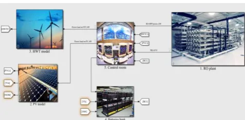
phase in this process is the pressure stage. At this stage, the feed pressure is increased to the appropriate level of membranes using the high-pressure pump (HPP), which ranges from 30 to 80 bar in the case of high feed salinity. Since the power consumption by the HPP is relatively high, an optimization model will be introduced in the next section to reduce the specific energy consumption (SEC). The HPP is fed from a hybrid renewable energy source (HRES) which is described in Fig. 2. Based on productivity, the plant is designed with a certain number of pressure vessels containing membrane elements. The hybrid energy source consists of PV panels, horizontal wind turbines (HWT), battery bank and converter. The size of PV panels, wind turbines and batteries is calculated using the PV-HWT-RO model as well as the total annual costs of the plant and the cost of producing fresh water with different plant capacities from 100 to 10000 m3 per day. As shown in Fig. 3, the PV-HWT-RO model consists of five major sub-systems with the following characteristics:
PV panel
Battery bank Wind turbine
Converter
AC DC
RO plant
Fig. 2. A schematic diagram of the hybrid renewable energy source supplying the RO plant.
Fig. 3. PV-HWT-RO simulation model using Matlab/Simulink.
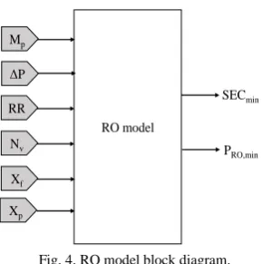
RO plant model: In this model, the productivity ranges from 100 to 10000 m3/day. The operating conditions, salinity, membrane type, recovery ratio, HPP efficiency, number of pressure vessels, number of membrane elements per vessel and other design criteria are determined. The model determines the power consumption by the HPP, the specific energy consumption and the required applied pressure across the membranes. PV model: In this model, various manufacturing manuals
(over 500 datasheets) are stored with different PV power ratings of 50 W to 320 W. The model allows the selection of appropriate PV panels and gives the main specifications based on the average solar radiation such as open circuit voltage, short circuit current, voltage at maximum power, current at maximum power, module efficiency and cost. HWT model: The horizontal wind turbine model design is
power from 1 kW to 50 kW and the average wind speed, then the model determines the main specifications of the selected wind turbine. These specifications include cut-in wind speed, rated speed, rotor diameter, rotor speed, hub height, rated voltage and unit cost.
Batteries bank: This model calculates the battery Wh storage, the battery Ah capacity and the number of batteries according to the battery voltage, efficiency, depth of discharge and battery cost.
Control room unit: This unit is responsible for calculating the total annual costs of RO plant, PV panels, wind turbines and batteries according to the productivity, plant life time and interest rate. It also calculates the unit product cost in $/m3 of fresh water and regulates the load distribution between PV and wind turbines. It has a splitter ratio from 0 to 1 while 0 means full loaded on PV and 1 means full loaded on WT. The splitter ratio can be controlled to show the load power fluctuations on both PV and WT relative to weather conditions variation. The PV-HWT-RO model is built and simulated using Matlab/Simulink.
A. Reverse Osmosis Mathematical Model [2], [7]
The feed flow rate to reverse osmosis membranes can be expressed by the following equation
. /RR M
Mf p (1)
where Mf, Mp and RR are the feed flow rate, permeate flow rate and recovery ratio, respectively. The fresh water (permeate) salinity is expressed by
. / )
( s t av p
p K A X M
X (2) where Xp, ks, At and Xav are the permeate salinity, salt permeability, total membrane area and average salinity, respectively. The salt permeability is given by
))). 273 ( 10 3 . 5 ( 062 . 0 ( 10 72 .
4 7 5
sea s T TCF FF
K (3)
where ks, FF, TCF, Tsea are the salt permeability, the membrane fouling factor, the temperature correction factor and seawater temperature, respectively. The temperature correction factor TCF is calculated by
)). 298 / 1 ) 273 /( 1 ( 3020
exp(
Tsea
TCF (4)
The concentrate (brine) flow rate can be calculated as .
p f
c M M
M (5) where Mc is the brine flow rate. The rejected salt concentration can be determined by
. / )
( f f p p c
c M X M X M
X (6)
where Xc, Xf are the concentrate and feed salt concentration, respectively. The membrane water permeability kw is calculated by )). 273 ( / ) 177 . 0 ( 685 . 18 ( 10 84 . 6 8 sea c w T X
K (7)
The net pressure difference across the membrane ∆P is expressed by
. )
/(
P Mp TCF Kw FF Ae Ne Nv (8) where Ae, Ne, Nv and ∆π are the membrane element area, number of membrane elements per vessel, number of pressure vessels and the net osmotic pressure across the membrane, respectively. The required power input for the RO high-pressure pump PRO is given by
). /( ) 2777 . 0
( f hpp
RO M P
P
(9)where ρ and ηhpp are the feed water density and the high-pressure pump efficiency, respectively. Finally, the specific energy consumption of the RO plant is calculated by
. / ) 24 (PRO Mp
SEC (10)
B. RO Optimization Model Formula
The objective of the RO optimization model shown in Fig. 4 is to minimize the total power consumption by the RO high-pressure pump and the specific energy consumption of the plant which in turn will reduce the overall costs and fresh water production cost.
). , , , , , , , , , , , ( hpp sea e p f e v p RO T FF A X X N N RR P M function SEC and P Minimize (11) Subject to 10000
100Mp (12) 45000
30000 Xf (13)
5 . 0 15
.
0 RR (14) 300
1Nv (15) 300
50Xp (16) 60
30P (17) The following design variables are supposed to be fixed as following C T and m kg FF mm A N sea hpp e e 20 / 1030 , 85 . 0 , 85 . 0 , 35 , 6 3 2
(18)
C. Proposed PV-HWT Model
The proposed PV model is provided through various manufacturing manuals (over 500 datasheets) with a different module power rating of 50 W to 320 W. As shown in Fig. 5, the user can assign the required PV power rating Pm and the average solar irradiance ∅S, then the model will determine the main characteristics of the specified panel such as open circuit voltage VOC, short circuit current Isc, voltage at maximum power Vmp, current at maximum power Imp, module efficiency
ηm and cost Cm. In addition, the total number of PV modules
Nm can be calculated as
. / m PV
m P P
respectively.
RO model p
M
SECmin ΔP
RR
v N
f X
p X
PRO,min
Fig. 4. RO model block diagram.
Moreover, the wind turbine model design is similar to the PV model design. The model is stored with more than 400 datasheets from different manufactures worldwide. The user can adjust the unit power Pu from 1 kW to 50 kW and the average wind speed in the site vav as shown in Fig. 6, then the model sets the main specifications of the selected wind turbine. These specifications include cut-in wind speed, rated wind speed, rotor diameter, rotor speed, hub height, rated voltage and unit cost. The total number of wind turbines Nu can be calculated from
. / u
WT P
P
Nu (20) where PWT and Pu are the total wind power and turbine unit power, respectively. Regarding the battery design, the total battery storage BSt can be calculated by
). /(
)
( t a b
t P OH N DOD
BS (21) where Pt, OH, Na, DOD and ηb are the total power consumption, operating hours per day, number of autonomy days and battery efficiency, respectively. The total batteries Ampere-hour Aht can be calculated by
. / b
t
t BS V
Ah (22) where Vb is the battery voltage. Then, the total number of batteries Nb can be calculated by
.
/ b
t
b Ah Ah
N (23) where Ahb is the battery Ampere-hour capacity. Finally, the power distribution on PV and WT can be expressed as
. ) 1
( t
PV spl P
P (24) .
t
WT spl P
P (25) where spl is the splitter ratio which ranges from 0 to 1. When (spl=0), this means that the RO plant is fully supplied by PV and when (spl=1), this means that full wind power is provided. The splitter ratio can be controlled to show the load variation on both PV and WT relative to weather conditions variation.
D. Cost Analysis of the PV-HWT-RO System [18]
The direct capital cost of the RO plant CDcan be estimated by the following equation
. ) 1000 500
( p
D M
C (26)
The cost of membrane elements purchase CM can be estimated by
. %) 60 % 50
( D
M C
C (27) The annual replacement cost of membrane elements CMR can be estimated by
PV model
m
P
VOC
ISC
Vmp
Imp
Cm ∅
Fig. 5. PV model block diagram.
WT model
u
P
Cut-in wind speed
Rotor speed
Unit cost Rated wind speed
Rotor diameter
Rated voltage Hub height
av
v
Fig. 6. Wind turbine model block diagram.
. %) 30 % 10
( M
MR C
C (28) The amortization factor AF is calculated by
). 1 ) 1 /(( ) ) 1 (
(
i i n i n
AF (29)
where i and n are the interest rate and the plant life time, respectively. The annual fixed charges CF can be estimated by
.
D
F AF C
C (30) The annual PV costs CPV can be calculated by
.
AF N C
CPV m m (31) where Cmand Nm are the PV module cost and the number of PV modules, respectively. The annual WT costs CWT can be calculated by
.
AF N C
CWT u u (32) where Cu and Nu are the cost of wind turbine unit and the number of wind turbines, respectively. The annual total batteries cost CTB is calculated by
.
AF N C
CTB b b (33) where Cb and Nb are the battery unit cost and number of batteries, respectively. The annual total costs of the plant Ct
. &M O TB WT PV F MR
t C C C C C C
C (34)
where CO&Mis the annual operation and maintenance cost of the plant. Finally, the unit water product cost Cw can be calculated by
). 365
/(
C M LF
CW t p (35) where LF is the load factor of the plant. All the above cost equations can be simulated in the control room subsystem at different plant capacities from 100 to 10000 m3/day. The system is designed and simulated using Matlab/Simulink assuming LF=0.85, i=0.05 and n=20 years.
III. SIMULATION RESULTS AND DISCUSSIONS
A. Effect of Varying the Recovery Ratio
By increasing the recovery ratio from 0.15 to 0.5, the SEC decreases from 7.6 to 3.2 kWh/m3 as shown in Fig. 7(a) and the power consumed by RO-HPP is reduced from 32 to 14 kW as shown in Fig. 7(b) at Mp = 100 m3/d, Nv = 2 and feed salinity of 30000 ppm. While the net pressure across membranes increases from 36 to 51 bar as described in Fig. 7(c), and the fresh water salinity also increases from 220 to 265 ppm. Therefore, the recovery ratio should not be significantly increased to keep ΔP and Xpwithin limits.
(a) (b)
(c) (d)
Fig. 7. Effect of varying RR on (a) SEC (b) PRO (c) ΔP and (d) Xp at Mp =100 m3/d, N
v= 2 and Xf = 30000 ppm.
(a) (b)
(c) (d)
Fig. 8. Effect of varying Nvon (a) SEC (b) PRO (c) ΔP and (d) Xp at Mp =500 m3/d, RR = 0.4 and X
f= 30000 ppm.
(a) (b)
(c) (d)
Fig. 9. Effect of varying Xfon (a) SEC (b) PRO (c) ΔP and (d) Xp at Mp =100 m3/d, Nv = 2 and RR = 0.4.
B. Effect of Varying the Number of Pressure Vessels
By increasing the number of pressure vessels, both SEC and power consumption are reduced to 3.5 kWh/m3 and 70 kW, respectively as shown in Fig. 8(a) and Fig. 8(b). This is due to the reduction in feed pressure with the increase of vessels as shown in Fig. 8(c). However, it can be observed that the permeate salinity Xp increases by increasing Nv as shown in Fig. 8(d). So, the optimum number of vessels will be obtained from the optimization model design of the RO at different plant capacities in order to maintain salinity within the limits (less than 300 ppm) and have the lowest SEC.
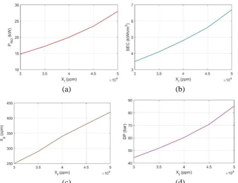
C. Effect of Varying the Feed Salinity
Fig. 9(a) and 9(b) show the effect of increasing seawater salinity from 30,000 ppm to 50,000 ppm on SEC and HPP power consumption at 100 m3/d productivity. The SEC increases from 3.5 kWh/m3 at Xf= 30000 ppm to 6.7 kwh/m3 at 50000 ppm of feed salinity. The power consumption also increases from 15 kW to 30 kW, where HPP requires high pressure to drive the highest salt water through membranes.
Fig. 9(c) and 9(d) illustrate that feed pressure and permeate salinity have a significant increase at higher feed salinity. Moreover, the SEC can be reduced by increasing Nv or decreasing RR. So, optimum values for Nv and RR are calculated at different feed salinities.
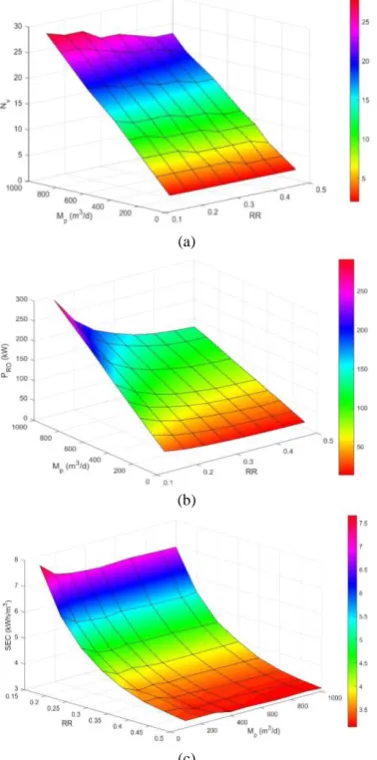
D. Optimization Results of RO Model
The results of the optimum values of number of pressure vessels Nv, power consumption by RO-HPP and SEC are shown in Fig. 10 based on the constraints of 100 ≤ Mp ≤ 1000 m3/d, 0.15 ≤ RR≤ 0.5 and Xf = 30000 ppm. The optimum number of pressure vessels ranges from 2 to 28 as shown in Fig. 10(a) of a plant capacity ranging from 100 to 1000 m3/day. It can be observed that by increasing the recovery ratio at a certain productivity, the number of vessels will be reduced to maintain pressure and permeate salinity within the required limits. With the increase in RR, a slight decrease in both power consumption and SEC occurs at small capacity, while a relative decrease occurs at high capacity as shown in Fig. 10(b) and Fig. 10(c). Finally, PRO ranges from 13 to 300
to 45000 ppm. The results of optimum values for Nv, PRO and
the SEC are illustrated in Fig. 11 at RR = 0.3 and variable productivity up to 10000 m3/d. Fig. 11(a) shows that Nv ranges from 2 to 230 and from 2 to 160 when salinity is 30000 and 45000 ppm, respectively. This means that high salt concentration plants require less number of vessels to produce the same amount of fresh water. However, both PRO and SEC
are relatively increased by increasing feed salinity due to increased pressure. As shown in Fig. 11(b), the power ranges from 18 to 1490 kW and 25 to 2480 kW at 30000 and 45000 ppm of feed salinity, respectively. While, the SEC is between 4 and 6.7 kWh/m3 at 30000 and 45000 ppm, respectively, as shown in Fig. 12(c).
(a)
(b)
(c)
Fig. 10. Results of the optimum values for (a) Nv (b) PRO and (c) SEC at Xf= 30000 ppm, 0.15 ≤ RR≤ 0.5 and 100 ≤ Mp≤ 1000 m3/d.
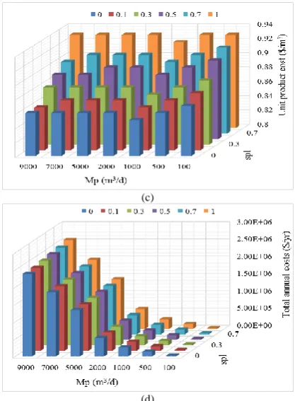
E. PV-HWT Model Results
The results of PV panel, wind turbine and battery specifications are summarized in Table I.
Based on the 250 W PV panel and 1000 W/m2 solar irradiance, the model gives the main characteristics of the panel, its life time and cost. With respect to average wind speed of 11 m/s in the site and 10 kW wind turbine power rating, the model provides the most suitable unit, its specifications, life time and cost. By simulating the model using these specified units under variable load conditions, it can calculate number of PV modules, number of wind
turbines, total annual costs and the unit cost of fresh water.
(a)
(b)
(c)
Fig. 11. Results of the optimum values for (a) Nv (b) PRO and (c) SEC at RR =
0.3, 30000 ≤ Xf≤ 45000 ppm and Mp≤ 10000 m3/d.
(a)
(c)
(d)
Fig. 12. Results of (a) number of wind turbines, (b) number of PV modules,
(c) unit product cost and (d) total annual costs at variable load conditions and splitter ratio ranging from 0 to 1 when Xf= 30000 ppm and RR = 0.5.
TABLEI:SPECIFICATION RESULTS OF THE PV-WTMODEL
PV module specifications
Modul e power
(W) Open circuit voltag
e (V) Short circuit current (A)
Voltage at maximum power (V)
Current at maximu m power
(A)
Module efficien
cy (%) Unit cost ($)
Life time (yr)
250 37.7 8.85 30.5 8.2 15.3 250 20
WT unit specifications
Unit power
(kW) Cut-in
wind speed (m/s)
Max. wind speed (m/s)
Rated AC voltage (V)
Hub height
(m)
Rotor speed (rpm)
Unit cost ($)
Life time (yr)
10 3 11 220 9 0 - 400 3000
0 20
Battery unit specifications
Battery voltage (V)
Battery capacit
y (Ah) Depth of discharg
e (%)
Battery efficiency
(%)
Battery
cost ($) Life time (yr)
12 100 80 75 110 5
By varying the splitter control ratio (spl) from 0 to 1, the load power fluctuates between the PV panels and the wind turbines. The economic results are shown in Fig. 12 under variable load capacity ranging from 100 to 10000 m3/d. When spl = 0 (full PV loaded), the number of PV modules ranges from 55 to 4600 panels with total annual costs ranging from 2.7e+04 to 2.4e+06 $/yr, and the unit product cost is about 0.86 $/m3. However, at spl = 1 (full WT loaded), the number of wind turbines ranges from 2 to 120 unit with total annual costs ranging from 3e+04 to 2.5e+06 $/yr, and the unit product cost is about 0.93 $/m3. It can be seen from Fig. 12(c), that the unit product cost is very close to 0.86 and 0.93 $/m3 for any amount of water production and different loading percentage. Also, the total annual costs are almost constant at constant capacity whether the load fluctuates between PV panels and wind turbines as shown in Fig. 12(d). For a reliable
design, the splitter ratio should be chosen between 0 and 1 (hybrid PV and WT source) according to the weather conditions in the site and the land area available for PV modules and wind turbines.
IV. MODEL VALIDATION
The developed model is validated by comparing the simulation results with the actual data of the desalination plant [6] in Matrouh, Egypt as a case study. The comparison show good results for power consumption, SEC and unit product cost as shown in Table II.
TABLEII:COMPARISON RESULTS OF THE DEVELOPED MODEL WITH
MATROUH PLANT
Variable Matrouh plant Developed
model
Plant capacity, m3/day 1200
Feed salinity, ppm 34000
Recovery ratio 0.45
Number of pressure vessels 5 6
Number of elements/vessel 4 5
Pressure, bar 35 37
Power consumption, kW 280 284
Specific energy consumption,
kWh/m3 4.7 4.65
Unit product cost, $/m3 1.25 1.13
V. CONCLUSIONS
A techno-economic study of a seawater reverse osmosis desalination plant fed by hybrid renewable PV and wind energy sources is presented. The main conclusions of this work are
Studying the effect of different operating conditions such as feed salinity, recovery ratio and the number of pressure vessels on the specific energy consumption of the plant. Designing an optimization model which gives the
optimum SEC based on the number of vessels and recovery ratio for a wide range of productivity from 100 to 10000 m3/day and different feed salts concentration. Designing a new model for PV panels and wind turbines
based on the storage of various manufacturing datasheets of different PV panels and WT power ratings. The model calculates the total annual costs under variable load conditions and the cost of fresh water production. Regulating the power distribution between PV and WT
sources using the splitter control ratio.
Validating the model by comparing the simulation results with the actual data of Matrouh desalination plant.
CONFLICT OF INTEREST
The authors declare no conflict of interest. AUTHOR CONTRIBUTIONS
approved the final version.
REFERENCES
[1] A. Lamei, P. Zaag, and E. Münch, “Basic cost equations to estimate unit production costs for RO desalination and long-distance piping to supply water to tourism-dominated arid coastal regions of Egypt,”
Desalination, vol. 225, pp. 1-12, 2008.
[2] A. Nafey and M. Sharaf, “Combined solar organic Rankine cycle with reverse osmosis desalination process: Energy, exergy, and cost evaluations,” Renewable Energy, vol. 35, pp. 2571-2580, 2010. [3] M. Wilf and C. Bartels, “Optimization of seawater RO systems
design,” Desalination, vol. 173, pp. 1-12, 2005.
[4] G. Kyriakarakos, A. Dounis, K. Arvanitis, and G. Papadakis, “Design of a fuzzy cognitive maps variable-load energy management system for autonomous PV-Reverse osmosis desalination systems: A simulation survey,” Applied Energy, vol. 187, pp. 575-584, 2017.
[5] D. Zejli, A. Ouammi, R. Sacile, H. Dagdougui, and A. Elmidaoui, “An optimization model for a mechanical vapor compression desalination plant driven by a wind/PV hybrid system,” Applied Energy, vol. 88, pp. 4042–4054, 2011.
[6] A. Hossam-Eldin, A. Elnashar, and A. Ismaiel, “Investigation into economical desalination using optimized hybrid renewable energy system,” Elec. Power and Energy, vol. 43, pp.1393-1400, 2012. [7] M. Laissaoui, P. Palenzuela, M. Sharaf, D. Nehari and D.
Alacron-Padilla, “Techno-economic analysis of a stand-alone solar desalination plant at variable load conditions,” Applied Thermal
Engineering, vol. 133, pp. 659–670, 2018.
[8] E. Mohamed, G. Papadakis, E. Mathioulakis, and V. Belessiotis, “A direct coupled photovoltaic seawater reverse osmosis desalination system toward battery-based systems-a technical and economical experimental comparative study,” Desalination, vol. 221, pp. 17-22, 2008.
[9] A. Helal, S. Al-Malek, and E. Al-Katheeri, “Economic feasibility of alternative designs of a PV-RO desalination unit for remote areas in the United Arab Emirates,” Desalination, vol. 221, pp. 1-16, 2008. [10] D. Manolakos, E. Mohamed, I. Karagiannis, and G. Papadakis,
“Technical and economic comparison between PV-RO system and RO-Solar Rankine system. Case study: Thirasia island,” Desalination, vol. 221, pp. 37-46, 2008.
[11] G. Ahmad, and J. Schmid, “Feasibility study of brackish water desalination in the Egyptian deserts and rural regions using PV systems,” Energy Conversion and Management, vol. 43, pp. 2641–2649, 2002.
[12] E. Tzen, K. Perrakis, and P. Baltas, “Design of a standalone PV-desalination system for rural areas,” Desalination, vol. 119, pp. 327-334, 1998.
[13] C. Liu, W. Xia, and J. Park, “A wind-driven reverse osmosis system for aquaculture wastewater reuse and nutrient recovery,” Desalination, vol. 202, pp. 24-30, 2017.
[14] I. Pestana, F. Latorre, C. Espinoza, and A. Gotor, “Optimization of RO desalination systems powered by renewable energies. Part I: Wind energy,” Desalination, vol. 160, pp. 293-299, 2014.
[15] D. Dehmas, N. Kherba, F. Hacene, N. Merzouk, M. Merzouk, H. Mahmoudia, and M. Goosen, “On the use of wind energy to power reverse osmosis desalination plant: A case study from Ténès (Algeria),” Ren. and Sust. Energy, vol. 15, pp. 956–963, 2011. [16] L. Rodríguez, V. Ternero, and C. Camacho, “Economic analysis of
wind-powered desalination,” Desalination, vol. 137, pp. 259–265, 2011.
[17] V. Romero, L. García, and C. Gómez, “Thermoeconomic analysis of wind powered seawater reverse osmosis desalination in the Canary Islands,” Desalination, vol. 186, pp. 291–298, 2005.
[18] A. Nafey, M. Sharaf, and L. Rodríguez, “Thermo-economic analysis of a combined solar organic rankine cycle-reverse osmosis desalination
process with different energy recovery Configurations,” Desalination, vol. 261, pp. 138-147, 2010.
Copyright © 2019 by the authors. This is an open access article distributed under the Creative Commons Attribution License which permits unrestricted use, distribution, and reproduction in any medium, provided the original work is properly cited (CC BY 4.0).
Ahmed A. Hossam-Eldin got his B.Sc (EE) distinction with honors, the M.Sc from Alexandria University on 1965 and 1969 respectively and the Ph.D from Heriot-Watt University, Edinburgh, U.K on 1972, where he worked as a staff member. He was promoted to Professor of Electrical Materials and Power Engineering in Alexandria University. His fields of interest are: electromagnetic interference, cryogenic & superconducting cables, partial discharges, and breakdown in dielectrics, distribution systems, renewable energy, biomass and biodiesel, utilization of renewable energy in desalination, cathodic protection and lightning protection. He published more than 300 articles in top refereed journals and published 5 books. He patented some of his work. He received top national and international awards for his contribution to his society and the achievement to the world. He supervised 135 Postgraduate students for Ph.D and M.Sc. He is the PI for 30 research projects. He was a visiting professor to Universities in France, Southampton, Edinburgh, Zimbabwe, King Abdelaziz (S.A), Kuwait and Philips Dodge Cable co. USA.
Kamal A. Abed was born in Giza, Egypt, on January 14, 1955. He received the B.Sc. degree from Suez Canal University, Egypt, the M.Sc. degree from Cairo University, Egypt, and the Ph.D. degree from Warsaw University of Technology, Poland, in mechanical power engineering in 1978, 1986, and 1991, respectively. He is a professor of power and energy in 2002. From 2003 to 2010, He was the head of Mechanical Engineering Department, National Research Centre (NRC), Cairo, Egypt. He was the chair of Energy Resources and Environmental Engineering Department, Egypt-Japan University of Science and Technology (E-JUST), Alexandria, Egypt in 2010. He was the head of Scientific Instruments Centre, Cairo, from 2010 to 2015. From 2012 to 2015, He was the head of Engineering Research Division, National Research Centre (NRC), Cairo, Egypt. He is currently an Emeritus Professor of Power and Energy, in the Mechanical Engineering Department, NRC, Cairo, Egypt.
Karim H. Youssef received the B.Sc., M.Sc., and Ph.D. degrees in electrical engineering from Alexandria University, Alexandria, in 2003, 2005, and 2009, respectively. He is an associate professor in the Electrical Engineering Department, Faculty of Engineering, Alexandria University. His current research interests include power system design, control and automation, power electronics applications, renewable energy, and smart grid. Dr. Youssef was the recipient of the Egyptian Government Award for his Ph.D. dissertation.