An inventory model for deteriorating items with time dependent demand using triangular trident fuzzy numbers

(1)

AN INVENTORY MODEL FOR DETERIORATING ITEMS WITH TIME DEPENDENT

DEMAND USING TRIANGULAR TRIDENT FUZZY NUMBERS

1_{Department of Mathematics, Avinashilingam Institute for Home Science and Higher Education for Women,}

2_{Department of Mathematics Jayaraj Annapackiam College for Women,} A R T I C L E I N F O

INTRODUCTION

Inventory is very essential in business such as manufacturing goods, selling goods etc. The inventory level should be maintained to avoid loss and increase the business profit. Uncertainties and imprecision is inherent in real inventory problems. This can be approached by probabilistic methods. But there are uncertainties that cannot be appropriately treated by usual probabilistic models. To define inventory optimization tasks in such environment and to interpre optimal solution, fuzzy set theory is considered as more convenient than probability theory. Many researchers have done their research work in fuzzy inventory models by considering the parameters as fuzzy number and defined various methods to get optimum cost. In this research work we get better optimum solution when compared to previous available methods.

The structure of this paper is as follows: Section 2 gives preliminaries that are essential for our work. Section 3 discusses an inventory model in crisp and fuzzy sense. Section 4 compares crisp model and fuzzy model (triangular trident fuzzy number) using a numerical example. Section 5 gives sensitivity analysis. Finally section 6 concludes this research paper.

International Journal of Current Advanced Research

ISSN: O: 2319-6475, ISSN: P: 2319-6505,

Available Online at www.journalijcar.org

Volume 8; Issue 07 (B); July 2019; Page No.

DOI: http://dx.doi.org/10.24327/ijcar.2019

which permits unrestricted use, distribution, and reproduction in any medium, provided the original work is properly cited. Article History:

Received 12th April, 2019

Received in revised form 23rd May, 2019 Accepted 7th_{June, 2019}

Published online 28th July, 2019

Key words:

Triangular trident fuzzy numbers, deteriorating items, fuzzy inventory, Defuzzification

*Corresponding author: Rama B

Department of Mathematics, Avinashilingam Institute for Home Science and Higher Education for Women,

Coimbatore

AN INVENTORY MODEL FOR DETERIORATING ITEMS WITH TIME DEPENDENT

DEMAND USING TRIANGULAR TRIDENT FUZZY NUMBERS

Rama B

1

_{and Michael Rosario G}

2

Avinashilingam Institute for Home Science and Higher Education for Women, Coimbatore

Jayaraj Annapackiam College for Women, Periyakulam, Tamil Nadu, India

A B S T R A C T

The aim of this research work is to find minimum cost and optimum time period in fuzzy inventory models. For this objective, the parameters in the inventory models are considered as triangular trident fuzzy numbers. Numerical example is worked out to explain the concept. Sensitivity analysis is also provided in this paper.

Inventory is very essential in business such as manufacturing goods, selling goods etc. The inventory level should be maintained to avoid loss and increase the business profit. inherent in real inventory problems. This can be approached by probabilistic methods. But there are uncertainties that cannot be appropriately treated by usual probabilistic models. To define inventory optimization tasks in such environment and to interpret optimal solution, fuzzy set theory is considered as more convenient than probability theory. Many researchers have done their research work in fuzzy inventory models by considering the parameters as fuzzy number and defined cost. In this research work we get better optimum solution when compared to previous

structure of this paper is as follows: Section 2 gives preliminaries that are essential for our work. Section 3 discusses crisp and fuzzy sense. Section 4 compares triangular trident fuzzy number) using a numerical example. Section 5 gives sensitivity analysis. Finally section 6 concludes this research paper.

Preliminaries

Definition

Let X be a nonempty set. Then a fuzzy set A in X (ie., a fuzzy subset A of X) is characterized by a function of

X



[0,1]. Such a function µ function and for each xϵX ,

membership of x (membership grade of x) in the fuzzy set A. In other words, A fuzzy set

A

~

µA: X



[0,1]. Ғ(X) denotes the collection of all fuzzy sets in

X, called the fuzzy power set of X. Definition

A fuzzy set is a fuzzy number if it satisfies the following four conditions

1. It is a convex set 2. It is normalised

3. It is defined on the real number R 4. It is piecewise continuous

Definition (Triangular trident Fuzzy Number )

A fuzzy number A =(a1q, a2q, a

fuzzy number if its membership function is given by

International Journal of Current Advanced Research

6505, Impact Factor: 6.614

www.journalijcar.org

; Page No.19451-19456

//dx.doi.org/10.24327/ijcar.2019.19456.3755

Rama B and Michael Rosario G. This is an open access article distributed under the Creative Commons Attribution License, which permits unrestricted use, distribution, and reproduction in any medium, provided the original work is properly cited.

Department of Mathematics, Avinashilingam Institute for Home Science and Higher Education for Women,

AN INVENTORY MODEL FOR DETERIORATING ITEMS WITH TIME DEPENDENT

DEMAND USING TRIANGULAR TRIDENT FUZZY NUMBERS

Avinashilingam Institute for Home Science and Higher Education for Women,

Periyakulam, Tamil Nadu, India

The aim of this research work is to find minimum cost and optimum time period in fuzzy models. For this objective, the parameters in the inventory models are considered as triangular trident fuzzy numbers. Numerical example is worked out to explain the concept. Sensitivity analysis is also provided in this paper.

Let X be a nonempty set. Then a fuzzy set A in X (ie., a fuzzy subset A of X) is characterized by a function of the form µA :

[0,1]. Such a function µA is called the membership

ϵX ,



_A~

 

x

is the degree of membership of x (membership grade of x) in the fuzzy set A.

A

~

=





x

,



_A

 

x



/

x



X



where Ғ(X) denotes the collection of all fuzzy sets in X, called the fuzzy power set of X.

A fuzzy set is a fuzzy number if it satisfies the following four

It is defined on the real number R It is piecewise continuous

Definition (Triangular trident Fuzzy Number )

, a3q) is called triangular trident

fuzzy number if its membership function is given by

Research Article

(2)

An Inventory Model for Deteriorating Items with Time Dependent Demand using Triangular Trident Fuzzy Numbers



















































q

q q

q

q q

q

A

a

x

a

x

a

x

a

x

a

x

a

x

a

x

q

3 3

1

3 2

3 1

2 3

2

2 1

3 1

1 2

2

1 3

1

,

1 ,

,

0 ,

,

1 )

(



Definition 2.4.( α-cut for triangular trident Fuzzy number)

The α-cut of triangular trident fuzzy number Aq is the closed

interval



 q

A











a

q

a

q

a

q

a

q

a

3q

a

2q



3 2 1 2 3

2







,







, α



[

0 ,

1 ]

.

Definition 2.5 (Signed distance method)

The formula for defuzzifying triangular trident fuzzy number using signed distance method is

R=

_

















1

0

2 3 3 2 1 2 3 2

2

1 



a

d

a

=

1

0 2 3 4 2

1 2 4 2

4 )

(

4 )

(

2

1 













_





a



=

8

2

₂ ₃

1

a



Definition (Graded Mean Integration Representation method)

The formula for defuzzifying using gradient mean integration representation method is

R=

_

















1

0

2 3 3 2 1 2 3

2

)

(

2

1 



a

d

a

=









1

0 2 3 5 2 2 1 2 5 2 2

5

2

5

2

1 



















a



=

10

3

₂ ₃

1

a



Inventory model in crisp and fuzzy sense

Assumptions

1. The inventory system involves production of single item.

2. Lead time is zero and shortages are not allowed. 3. Demand is time dependent.

4. Replenishment is instantaneous. Notations

A - set up cost per cycle

A

~

- fuzzy set up cost

θ - deterioration rate independent of time



~

- fuzzy deterioration rate independent of time T - cycle length

P - production rate

P

~

- fuzzy production rate

h - holding cost per unit per unit time

h

~

- fuzzy holding cost per unit per unit time d - ` deterioration cost per unit per unit time

d

~

- fuzzy deterioration cost per unit per unit time D - demand rate which depends exponentialy over time

D

~

- fuzzy demand rate t1 - duration of production

I1(t) - inventory level at time t, 0≤t≤t1

I2(t) - inventory level at time t, t1 ≤ t ≤ T

C - total cost for the period [0,T]

C

~

- fuzzy total cost for the period [0,T]

C

d

_F

~

- defuzzified value of

C

~

Description of Inventory model in crisp sense

At t = 0, the inventory level is zero and it increases in [0,t1]

due to the production at the constant rate P.

At t = T again it reaches the inventory level zero. This is due to demand and deterioration of the item. This can be represented by the following figure 1

(3)

For 0 ≤ t ≤ t1

The differential equation governing the situation is

) ( )

( ₁

1 t P D I t

I dt d



    

 I t P

t I dt d ) ( ) ( ₁

1  Ke

-λt

, where K is the initial demand

and λ is the decreasing rate of demand. K > 0 and 0 < λ < θ t Ke P t I t I dt

d _ 

   () ) ( 1 1

Now apply the initial condition I1(t) =0 when t = 0 we get





(1 )

) ( 1 t t t e P e e K t

I   







       

For t1 ≤ t ≤ T

The differential equation governing the above condition is

 

 ()

)

( 2

2 t I t

I dt

d

 Ke-λt , where K is the initial demand and λ is the decreasing rate of demand. K > 0 and 0 < λ < θ. The solution of the linear equation after applying the condition I2 (t)= 0 at t = T is

Holding cost can be calculated by using the formula

















_

1 2 0 0 2 1

(

)

(

)

.

t t

dt

t

I

dt

t

I

h

C

H

we get





                 1 1 1 1 t P e K h T      

The deteriorating cost can be found out by the formula

















_

1 1 0 2

1

(

)

(

)

t T t

dt

t

I

dt

t

I

d

DC







_































d

K

1

1 e

T

Pt

₁









Total cost can be defined as



A

HC

DC



T

C



1 







_             P T K d h KT d h A T C t Total 2 2 2 1 2 2 1

cos   ---(1)

[9] The optimum value of T can be found out by differentiating with respect to T





0 2 1

2 2 3

2

2  

               T A T C and P K K d h T A T C  .

Now equate the first derivative to zero to obtain optimum time period T*





0

1

2





















P

K

d

h

T

A





















P

K

d

h

A

T

1

2 )

(

*



---(2)

Description of Inventory model in fuzzy sense Triangular trident fuzzy number

It is not always possible to define certain parameters with certainty for which we fuzzify some parameters A , h, d , θ , P , D , K.

We consider triangular trident fuzzy numbers for the above parameters as



₁

,

₂

,

₃



~

a

A



,



1

,

2

,

3



~

h





1

,

2

,

3



~

d



,



1

,

2

,

3



~





,



₁

,

₂

,

₃



~

p

P



,



1

,

2

,

3



~

d

D



,



1

,

2

,

3



~

k

K



Therefore, (1) becomes

Ci=





_



















i i i i i i i i i i

P

T

K

d

h

T

K

d

h

A

T

₄ 2 2 2

2

1

2

1 



, i =

1, 2, 3

To find the optimum value , we have to differentiate the above equation with respect to T









i i i i i i i i i i i

P

K

d

h

K

d

h

T

A

C

dt

d













4 2 2

2

1

2

1 )

(



, i

= 1,2,3 and ₂ ₃

2

2 )

(

T

A

C

dt

d

i



, i = 1,2,3

Now defuzzifying using signed distance method



1

2

2 3



8

1 ~

c

C

d

_F

























dt

dc

dt

dc

dt

dc

C

d

dt

d

F 1

2

2 3

8

1 ~





















2 3 2 2 2 2 2 1 2 2

2

8

1 ~

dt

c

d

dt

c

d

dt

c

d

C

d

dt

d

F

















3 3 3 2 3

1

2 ₂

2

8

1 T

a

T

a

T

a

3 3 2 1

4

2 T

a





_{which is greater than zero .}

Therefore we get the minimum total cost.

Now let us find optimum solution of total cost by putting



d

C



dt

d

F

~

=0

























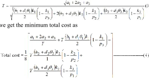
1 ₂2 3

1 2 3 3 3 3 2 2 2 2 2 2 3 2 1 1 1 1 3 3 3 3 2 2 2 2 1 1 1 1 2 2 1 2 2 2 1 2 1 2 2 2 1 T a a a p k d h p k d h p k d h k d h k d h k d h                    



T T t t



e

K

t

I

   

(4)

we get the minimum total cost as

Similarly defuzzifying using graded mean integration method, we get the optimum time period and minimum total cost as

Numerical Example

Crisp Model

Suppose A = 54, h = 8, θ = 0.010, P = 550, d = 1.5, K = 500 By using the formula (1) and (2), we get T* = 0.54

And total cost C = 198.37 Fuzzy Model

Signed Distance method

A = (20,26,32), h = (4,6,8), θ=(0.002,0.006,0.010), P =(500,550,600), d =(1,1.3,1.6) K=(450,500,550)

Using (3) and (4) we get T*= 0.6 and total cost = 42.495 Graded mean Integration method

A = (20,26,32), h = (4,6,8), θ=(0.002,0.006,0.010), P =(500,550,600), d =(1,1.3,1.6) K=(450,500,550)

Using (5) and (6) we get the optimum solution as T*= 0.56 and total cost = 46.41

Sensitivity Analysis

The following table shows the effect of change of each parameter in (3),(4), (5) & (6)

From the Table 1, we observe that increase in setup cost increases the time period and the total cost. Table 2 shows that if the deterioration cost increases then there is no rapid change in the time period and total cost.

(20,26,32) (30,34,38) (50,52,54) (60,70,80) Graded mean method

T(years) 0.56 0.6406 0.7922 0.9191 Signed distance method

T(years) 0.6 0.6997 0.8654 1.004 0

0.2 0.4 0.6 0.8 1 1.2

TI

M

E

P

ERI

OD

OPTIMUM TIME PERIOD FOR DIFFERENT VALUES OF FUZZY SETUP COST

Table 1

A

~

Graded mean method

Signed distance method T(years) Total

cost T(years)

Total cost

(20,26,32) 0.56 46.41 0.6 42.50

(30,34,38) 0.6406 53.08 0.6997 48.59

(50,52,54) 0.7922 65.64 0.8654 60.09

(60,70,80) 0.9191 70.25 1.004 69.72

Table 2

d

~

Graded mean method Signed distance method T(years) Total

cost T(years)

Total cost

(1,1.6,2.2) 0.6406 53.08 0.6999 48.58

(1,1.3,1.6) 0.6406 53.08 0.6997 48.59

(1.3,1.7,2.1) 0.6405 53.08 0.6997 48.59

(2,2.5,3) 0.6404 53.09 0.6997 48.59

Table 3



~

Graded mean method

Signed distance method T(years) Total

cost T(years) Total

cost

(0.002,0.006,0.010) 0.6406 53.08 0.6997 48.59

(0.003,0.006,0.009) 0.6405 53.09 0.6996 48.6

(0.005,0,010,0.015) 0.6403 53.10 0.6995 48.61

(0.008,0.015,0.022) 0.6401 53.12 0.6993 48.62

Table 4

K

~

_T(years)Graded mean method _{Total cost} Signed distance method _T(years) _{Total cost}

(450,500,550) 0.6406 53.08 0.6997 48.59

(400,425,450) 0.3592 94.66 0.3638 93.45

(350,410,470) 0.3554 95.65 0.3630 93.65

(200,230,260) 0.2935 115.83 0.2942 115.56

Table 5

h

~

_T(years)Graded mean method _{Total cost} Signed distance method _T(years) _{Total cost}

(2,7,12) 0.8086 42.05 1.16 29.26

(4,6,8) 0.6406 53.08 0.6997 48.59

(3,9,15) 0.6777 50.17 0.9069 37.49

(10,14,18) 0.4077 83.38 0.4396 77.35

Table 6

P

~

T(years) Graded mean method Total cost Signed distance method T(years) Total cost

(500,550,600) 0.6406 53.08 0.6997 48.59

(550,575,600) 0.4573 74.35 0.4695 72.41

(600,700,800) 0.3019 112.62 0.3078 110.48

(5)

Graphical representation of Table 1

Since the deterioration rate is very minimum in our example problem, there is not much change in the time period and total cost if the deterioration rate of material increases which is depicted in Table 3. If the production is l

demand is less then there is huge rise in total cost and the time period of one cycle is very minimum which is shown in Table 4 and Table 6. Table 5 shows that if the holding cost of material for placing in the inventory increases then the c incurred for the cycle also increases.

(20,26,32) (30,34,38) (50,52,54)

Graded mean

method Total cost 46.41 53.08 Signed distance

method Total cost 42.5 48.59 20

30 40 50 60 70 80

To

tal Co

st

OPTIMUM TOTAL COST FOR DIFFERENT VALUES OF FUZZY SETUP COST

(1,1.6 ,2.2)

(1,1.3 ,1.6)

Graded mean method

T(years) 0.6406 0.6406 0.61

0.63 0.65 0.67 0.69 0.71

Ti

me

P

erio

d

OPTIMUM TIME PERIOD FOR DIFFERENT VALUES OF

(1,1.6,2. 2)

(1,1.3,1. 6)

(1.3,1.7,

Graded mean method

Total cost 53.08 53.08 53.08

Signed distance method

Total cost 48.58 48.59 48.59 46

47 48 49 50 51 52 53 54

TOT

AL COST

OPTIMUM TOTAL COST FOR DIFFERENT VALUES OF

Table 1

Since the deterioration rate is very minimum in our example problem, there is not much change in the time period and total cost if the deterioration rate of material increases which is depicted in Table 3. If the production is large while the demand is less then there is huge rise in total cost and the time period of one cycle is very minimum which is shown in Table 4 and Table 6. Table 5 shows that if the holding cost of material for placing in the inventory increases then the cost

Table 2

Graphical representation of

(50,52,54) (60,70,80)

65.64 70.25

60.09 69.72

OPTIMUM TOTAL COST FOR DIFFERENT VALUES OF FUZZY SETUP COST

(1.3,1 .7,2.1 )

(2,2.5 ,3)

0.6405 0.6404

OPTIMUM TIME PERIOD FOR DIFFERENT

(1.3,1.7,

2.1) (2,2.5,3)

53.08 53.09

48.59 48.59

OPTIMUM TOTAL COST FOR DIFFERENT

(0.00 2,0.0 06,0. 010)

Graded mean method

T(years) 0.6406 0.6

0.62 0.64 0.66 0.68 0.7 0.72

TI

M

E

P

ERI

OD

(0.002,0 .006,0.0 10) Graded mean method

Total cost 53.08 Signed distance method

Total cost 48.59 46

48 50 52 54

TOT

AL

COST

0.6406

0.3592 _0.3554

0.2935

T(years)

Graded mean method

53.08 94.66 95.65

115.83

Total cost

Graded mean method

OPTIMUM TOTAL COST FOR DIFFERENT VALUES OF Graphical representation of Table 3

Graphical representation of Table 4 (0.00

3,0.0 06,0. 009)

(0.00 5,0,0 10,0. 015)

(0.00 8,0.0 15,0. 022)

0.6405 0.6403 0.6401

(0.002,0 .006,0.0

(0.003,0 .006,0.0 09)

(0.005,0 ,010,0.0 15)

(0.008,0 .015,0.0 22)

53.08 53.09 53.1 53.12

48.59 48.6 48.61 48.62

0.6997

0.3638 0.363 0.2942

T(years)

48.59 93.45 93.65

115.56

Total cost

(6)

(2,7,12) (4,6,8) (3,9,15)

Graded mean method T(years)

0.8086 0.6406 0.6777

Signed distance method T(years)

1.16 0.6997 0.9069

0 0.2 0.4 0.6 0.81 1.2 1.4

Ti

m

e Perio

d

OPTIMUM TIME PERIOD FOR DIFFERENT VALUES OF

(2,7,12) (4,6,8) (3,9,15)

Graded mean

method Total cost 42.05 53.08 50.17

Signed distance

method Total cost 29.26 48.59 37.49 20

30 40 50 60 70 80 90

To

tal Co

st

0.6406 0.6997

0.4573 0.4695

0.30190.2946 0.3078

T(years) T(years)

Graded mean method Signed distance method

53.08 74.35

112.62 115.42

Total cost

Graded mean method Signed distance method

ing Items with Time Dependent Demand using Triangular Trident Fuzzy Numbers

Table 5

Table 6

CONCLUSION

In this paper an inventory model is considered. The description for the model is given in crisp and fuzzy environment. The crisp model of the problem was already discussed in [9] . In Paper [9], the fuzzy numbers we

trapezoidal fuzzy numbers. In our present paper, we used triangular trident fuzzy number. Signed distance method and graded mean integration method are used for defuzzification. We observe that, we obtain minimum total cost and opt time period while using Triangular trident fuzzy number.

References

1. Dutta D and PavanKumar., Fuzzy inventory model without shortages using trapezoidal fuzzy number with sensitivity analysis, IOSR

2012, 32- 37.

2. Hadely G, Whitin T M ., Analysis of inventory systems, Prentice hall,1963.

3. Harris F., Operations and Cost, AW Shaw co. Chicago 1915.

4. Jaggi C K, Pareek S, Khanna A and Nidhi ., Optimal Replenishment policy for fuzzy Inventory model with Deteriorating items and under

under Inflationary conditions. Yugoslav

Operations Research,10,2016, 2298/YJOR150202002Y 5. Jain R., Decision making in the presence of fuzzy

variables, IIIE Transactions on systems, Man and Cybernetics, 6, 1976, 698

6. Kacpryzk J and Staniewski P., Long term inventory policy-making through fuzzy

Fuzzy sets and systems, 8 , 1982, 117

7. Kumar S and Rajput U S., Fuzzy Inventory model for Deteriorating items with Time dependent demand and partial backlogging, Applied Mathematics, 6,2015, 496 509.

8. Nanbendusen, BimanKantiNath, SumitSaha., A fuzzy Inventory model for deteriorating items based on different defuzzification techniques

of Mathematics and statistics, 6(3), 2016, 128

9. Rama B and Michael Rosario G ., An inventory model for deteriorating items with time dependent demand in both fuzzy and crisp sense,

International Research Journal

2018, 160-170.

10. Saha S and Chakraborty T. time dependent demand and shortages, IOSR Journal of Mathematics

54.

11. Trailokyanath Singh, HadibandhuPattanayak., An EOQ model for a Deteriorating item with time dependent demand exponentially declinin

permissible delay in payment, IOSR

Mathematics, 2, 7,2012, 30

12. Wilson R.,A scientific routine for stock control. Harvard Business review,13,1934,116

13. Zadeh,L.A., Fuzzy sets, Information control, 8, 338-353.

14. Zimmermann,H J., Using fuzzy sets in Operational Research, European Journal of Operations Research

13, 1983, 201-206.

(3,9,15) (10,14,1

8)

0.6777 0.4077

0.9069 0.4396

OPTIMUM TIME PERIOD FOR DIFFERENT VALUES OF

(3,9,15) (10,14, 18)

50.17 83.38

37.49 77.35

0.2989

OPTIMUM TIME PERIOD FOR DIFFERENT

48.59 72.41

110.48113.75

Total cost

ing Items with Time Dependent Demand using Triangular Trident Fuzzy Numbers

In this paper an inventory model is considered. The description for the model is given in crisp and fuzzy environment. The crisp model of the problem was already discussed in [9] . In Paper [9], the fuzzy numbers we used are triangular and trapezoidal fuzzy numbers. In our present paper, we used triangular trident fuzzy number. Signed distance method and graded mean integration method are used for defuzzification. We observe that, we obtain minimum total cost and optimum time period while using Triangular trident fuzzy number.

Dutta D and PavanKumar., Fuzzy inventory model without shortages using trapezoidal fuzzy number with sensitivity analysis, IOSR Journal of Mathematics, 4,

Whitin T M ., Analysis of inventory systems,

Harris F., Operations and Cost, AW Shaw co. Chicago

Jaggi C K, Pareek S, Khanna A and Nidhi ., Optimal Replenishment policy for fuzzy Inventory model with Deteriorating items and under allowable shortages under Inflationary conditions. Yugoslav Journal of

,10,2016, 2298/YJOR150202002Y Jain R., Decision making in the presence of fuzzy IIIE Transactions on systems, Man and

1976, 698-703.

Kacpryzk J and Staniewski P., Long term inventory making through fuzzy-decision making models., Fuzzy sets and systems, 8 , 1982, 117-132.

Kumar S and Rajput U S., Fuzzy Inventory model for Deteriorating items with Time dependent demand and ial backlogging, Applied Mathematics, 6,2015, 496-

Nanbendusen, BimanKantiNath, SumitSaha., A fuzzy Inventory model for deteriorating items based on different defuzzification techniques, American Journal

Mathematics and statistics, 6(3), 2016, 128-137. Rama B and Michael Rosario G ., An inventory model for deteriorating items with time dependent demand in both fuzzy and crisp sense, Mathematical Sciences, International Research Journal, 7, special issue 1,

Saha S and Chakraborty T., Fuzzy EOQ model with time dependent demand and deterioration with

Journal of Mathematics, 2, 2012,

46-Trailokyanath Singh, HadibandhuPattanayak., An EOQ model for a Deteriorating item with time dependent demand exponentially declining demand under permissible delay in payment, IOSR Journal of

, 2, 7,2012, 30-37.

Wilson R.,A scientific routine for stock control. Harvard Business review,13,1934,116-128.

Zadeh,L.A., Fuzzy sets, Information control, 8, 1965,

,H J., Using fuzzy sets in Operational