Robustness of Lord’s Formulas for Item Difficulty and Discrimination Conversions Between Classical and Item Response Theory Models

Teresa Dawber

W. Todd Rogers

and

Michael Carbonaro

Robustness of Lord’s Formulas for Item

Difficulty and Discrimination Conversions

Between Classical and Item Response

Theory Models

Lord (1980) proposed formulas that provide direct relationships between IRT

discrimination and difficulty parameters and conventional item statistics. The purpose of the present study was to determine the robustness of the formulas beyond the initial and restrictive conditions identified by Lord. Simulation and real achievement data were employed. Results from the simulation study indicate that the item discrimination parameters were recovered quite well for low to moderately discriminating items regardless of ability distribution, and the difficulty parameters were recovered quite well for the range typically found for achievement tests. Results of the real data were consistent with those found for the simulation study.

Lord (1980) a proposé des formules qui fournissent des rapports directs entre la

discrimination et les paramètres de difficulté de la théorie de la réponse d’item d’une part, et les modèles classiques portant sur les items d’autre part. L’objectif de la présente étude était de déterminer la robustesse des formules au-delà des conditions initiales et restrictives identifiées par Lord. Nous avons utilisé des données de rendement d’une étude en

simulation et d’une analyse de données réelles. Les résultats provenant de l’étude en simulation indiquent que les paramètres de discrimination d’item étaient assez bien recouvrés pour les items dont le pouvoir de discrimination était bas ou moyen,

indépendamment de la distribution des capacités, et que les paramètres de difficulté étaient assez bien recouvrés pour l’écart commun aux tests de rendement. Les résultats provenant des données réelles étaient compatibles avec celles de l’étude en simulation.

The field of psychometrics encompasses alternative models for performing test and item analyses. The classical test score theory (CTST) model, the foundation of which was provided by Spearman (1904), is the traditional means of con-ducting item and test analyses. The family of item response theory (IRT)

Teresa Dawber works as a psychometrician in the United States. Her primary responsibilities include operational work on state contracts for several K12 testing programs.

Todd Rogers is a professor and faculty member in the Centre for Research in Applied Measurement and Evaluation. His research interests are in psychometrics, large-scale assessments, and ethics in testing.

models, first introduced by Lord in 1952 for dichotomously scored items, was developed to circumvent the limitations of CTST. However, Lord (1980; Lord & Novick, 1968) proposed formulas that link the item difficulty and item dis-crimination indices of the CTST and the two-parameter IRT model under the conditions that ability is normally distributed and there is no guessing (Lord). One example in which these formulas can be profitably used is in the area of computer adaptive testing. The cost associated with obtaining large enough samples to use IRT to screen items for the needed item banks, Lord’s formulas, which can be used with smaller sized samples, could provide the information needed to screen items. Another is in the field testing of items that have been embedded in operational test forms in such a way as to have a multiple matrix sample design. The samples of students per item may not be sufficient to conduct IRT analyses. In this case, the Lord’s estimates may be sufficient to complete an item analysis of the embedded field test items to determine which of these items should be selected for a future operational form.

Lord’s Formulas

For item discrimination, to the extent that number correct score x is a measure of ability (θ), the biserial correlation between the item and test score (ρ′ix) is an approximation of the correlation between the item score and ability estimate (ρiθ). This association yields a relationship between the CTST biserial item-test correlation and the IRT discrimination index (ai) (Lord, 1980, p. 33):

ai =

_{√⎯⎯⎯⎯⎯⎯}

1 −ρ′ix2

The IRT item discrimination parameter and the CTST biserial correlation are approximately monotonic increasing nonlinear functions of each other. How-ever, Lord cautioned that the approximation is crude and may fall short be-cause (a) test score x contains errors of measurement whereas θ does not, and (b) x and θ may have differently shaped distributions.

Lord also proposed a monotonic relation between the IRT difficulty index (bi) and the CTST difficulty index (πi) when all items are equally discriminating (Lord, 1980, p. 33):

bi ≈ _ρ′γi ix

The difficult parameter bi is proportional to γi, the cut-point in the continuous normal distribution underlying the binary item that separates the proportion of incorrect answers (1 – πi) and the proportion of correct answers (πi). Both bi and

γi decrease as πi increases.

Using the formulas proposed by Lord and Novick (1968), Urry (1974) devel-oped a graphical method. He devised graphs that consisted of mapping a grid system to model the a- and b-parameters onto a coordinate system where the population point-biserial correlation, rather than the biserial correlation, was the ordinate and the population proportion passing an item was the abscissa. By plotting the data points for a given item using the conventional indices, the estimates of ai and bi may be interpolated. When there is no guessing, the graph is symmetric. When there is guessing, the graph is displaced to reflect inflation in the proportion passing the item and attenuation in the point-biserials through error due to guessing.

Urry (1974) proposed that the following four conditions needed to be met for effective application of the graphical method: (a) the latent trait is normally distributed; (b) the CTST indices are based on large samples (n=2,000) in order to approximate the set of parameters; (c) the items in the test must be homogenous (KR20≥ 0.90); and (d) the items in the test must be of sufficient number (k=80) for the point-biserial correlation between item and total test score to bear a close relationship to the correlation between the item score and the latent ability measured by the test. He then examined the graphical approx-imations using data from 4,950 examinee responses to 98 unscreened mathe-matics items from the Washington Pre-College Test Battery, a highly reliable test (KR20=0.93). Correlations between the estimated a- and b-parameters derived from the graphs and their corresponding maximum likelihood (ML) estimates were 0.89 and 0.97 respectively. Urry concluded that the correlation coefficients indicated a strong degree of accord between the graphical approx-imations and the ML estimates.

Subsequently, Schmidt (1977), in a theoretical paper, suggested that Urry’s (1974) graphical procedure tended to systematically underestimate ai and over-estimate ⏐bi⏐and the variance of bi because the point-biserial correlation be-tween the item score and the estimated latent trait (i.e., total test score), riθ^, was taken as an estimate of the point-biserial correlation between the binary item and the perfectly reliable latent trait, ρ^_iθ. Values of r_i‘θ^ are attenuated because of guessing on item i, and the unreliability of θ^. Schmidt pointed out that increased values of the biserial correlation imply larger a^i and smaller |b^i|. He argued that Urry’s four criteria would minimize rather than eliminate the bias noted.

-and b-values respectively. Jensema concluded that the graphical estimates were “surprisingly accurate” (p. 713). The correlations revealed that the agree-ment between the true parameters and the corresponding graphical estimates increased with increasing sample size and a greater number of test items, as initially suggested by Urry (1974). Jensema concluded that the graphical meth-od could be used as a convenient technique for examining the worth of an item pool for tailored testing.

Ree (1979) also conducted a simulation study to assess the effectiveness of the graphical method. The a- and b-values derived from the graphical method and the a- and b-values derived from three common computer programs (i.e., ANCILLES, LOGIST, OGIVIA) were correlated with true item parameters. Using the 3PL model, data were generated for an 80-item test for normally distributed, positively skewed, and uniformly distributed groups of 2,000 ex-aminees. The true item parameters represented real examination data and were normally distributed (Ma=0.95, SDa=0.28; Mb=0.16, SDb=0.93; Mc=0.20,

SDc=0.05). The correlations between estimated and true parameters revealed that the estimated b-values were more closely aligned to the true parameters than the estimated a-values. The correlations were equal to or higher than 0.90 for the b-parameters. Correlations of a-parameters and the values obtained from the graphical method were 0.32, 0.35, and 0.59 for the skewed, normal, and uniform ability distributions respectively. Correlations of a-parameters and the values obtained from the three computer programs also were variable across ability distributions. The lowest correlations, ranging from 0.44 to 0.57, were observed for the skewed data, whereas high correlations were found for the normal distribution (range of 0.83 to 0.84), and the uniform distribution (range of 0.87 to 0.90).

Although Lord’s formulas were used in the context of the three-parameter model, the studies suggest that the transformation procedures from the CTST item indices to the corresponding IRT item indices may have some promise under certain conditions. Taken together, the findings of these early studies indicated that the estimated b-parameters derived from the graphical method were highly correlated with true or ML estimates of b-values regardless of the shape of the ability distribution, whereas the correlations for the a-parameters were moderately to highly correlated.

Correlations were presented as evidence of the accuracy of the graphical method in the studies reviewed above. However, high correlations indicate only that sets of values are strongly linearly related; they provide no evidence of actual parameter recovery.

present study was to investigate the robustness of the formulas beyond the initial, restrictive conditions identified by Lord using fit statistics that assess degree of agreement.

Method

The robustness of Lord’s formulas was investigated using simulated data and actual achievement data. The simulated data were used to examine the be-haviors of the formulas under different experimental conditions where the population parameters were known. The achievement data were used to ex-amine the extent to which the simulation results were generalizable to real data.

Simulation Study

The research design for the simulation was a 3 x 3 x 2 x 3 (ability distribution-by-test length-by-item discrimination-by-sample size) fully crossed design. The levels of these factors were selected to represent realistic response data. Ability Distribution

Given that ability is probably not normally distributed for most groups of examinees (Lord, 1980), two skewed distributions were modeled as well the normal distribution. The skewed ability distributions were generated using the beta probability density function. The positively skewed distribution, defined as beta (2.9, 5.7), achieved an expected skewness of 0.40 and an expected kurtosis of –0.30; the negatively skewed distribution, defined as beta (5.7, 2.9), achieved an expected skewness of –0.40 and an expected kurtosis of –0.30. The beta distributions were linearly rescaled so that the mean and standard devia-tion of the distribudevia-tion of θs were 0 and 1 respectively.

Test Length

Three test lengths were employed: a short exam of 20 items, a moderate exam of 40 items, and a long exam of 80 items. The short and moderate exam lengths are consistent with lengths frequently found in psychological and educational applications (Seong, 1990; Yen, 1987). The longest exam is consistent with Urry’s (1974) requirement for the item-test point-biserial correlation to be a close approximation to the item-latent trait correlation.

Item Discrimination

Sample Size

Samples of 250, 500, and 1,000 examinees were randomly selected from the population of simulated examinees. The selection of these sample sizes is consistent with the selection of sample sizes considered in the previous studies in which the graphical procedure was used (see above).

Item Difficulty

Item difficulty, a random factor, was not considered in the present study. Instead, wanting to observe the effect of extreme values outside the normal range of –2 to 2, b-values were randomly selected from a normal distribution

(μ=0, σ=1) for all simulations. This procedure is consistent with the simulation

work conducted at ETS (D.L. Henderson-Montero, personal communication, May 2, 2003).

Data Generation

The four-step item response generation technique described by Harwell, Stone, Hsu, and Kirisci (1996) was used to create the data. Step 1 involved the genera-tion of true ability scores (θ). In Step 2, tests were created according to the test specifications (test length, a-parameters, and b-parameters). For each cell in the experimental design, a unique test was created by deriving new sets of a- and b-parameters consistent with the specifications for that cell. In Step 3, response probabilities of a population of 10,000 examinees to the k (20, 40, and 80) items based on the two-parameter IRT model were determined, producing a 10,000 x k matrix. The matrix of response probabilities was translated into a 10,000 x k data matrix of 0/1 responses in Step 4. Each response probability was com-pared with a random number drawn from a uniform distribution of values in the closed interval (0, 1). A 1 was assigned for that item if the response prob-ability was equal to or greater than the random number; otherwise 0 was assigned for that item.

Mathematica for Students (Version 4, Wolfram, 2000) was used to generate the response data matrices. LERTAP (Version 5, Nelson, 2000), an Excel applica-tion, was employed to obtain the classical item analyses and Lord’s estimation of the a- and b-parameters. Random sampling from the 10,000 examinees was performed with an Excel (Version 5) macro program.

Replications

The benefits of replicated over nonreplicated IRT simulation studies are the same as those observed in empirical studies; aggregating results over replica-tions produces more stable and reliable findings. The number of replicareplica-tions influences the precision of the estimated parameters. Therefore, increasing the number of replications is an attractive technique for reducing the variance error of estimated parameters (Harwell et al., 1996). In the present study, 100 random samples of 250, 500, and 1,000 examinees were drawn from the popu-lation for each experimental condition.

Achievement Data

1999a, 1999b). These examinations are high school graduation examinations, which contribute 50% toward students’ final course grades. Only the multiple-choice components of the exams were used, which comprised 48 items for the Biology exam and 70 items for the English exam.

The assumptions underlying the two-parameter IRT model were assessed. The shape of the Scree plot yielded by a principal component analysis showed a dominant first component and a difference between successive pairs of components that was small in comparison to the difference between the first and second components (Hambleton, Swaminathan, & Rogers, 1991), suggest-ing that each examination was essentially unidimensional (Nandakumar, 1994). Speed was not a factor; 24 (0.18%) English examinees and one (0.01%) biology examinee did not respond to the last three items.

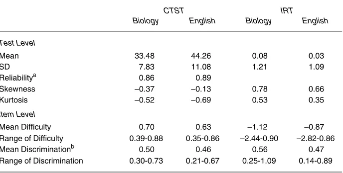
The psychometric properties of the biology and English examinations are provided in Table 1. The total test mean and CTST mean p-values reveal that the items were of moderate difficulty in both examinations. The observed score distributions for both exams were somewhat negatively skewed and playtykurtic. Item requirements for the exams include minimum and maxi-mum acceptable difficulty levels 0.30 and 0.85 respectively and a minimaxi-mum acceptable point-biserial correlation of 0.20 (Alberta Education, 1999). The mean biserial correlations met the criterion of 0.40 and above to be considered high (Nelson, 2001).

Examination of the IRT information revealed that the ability distributions for both exams were positively skewed and leptokurtic.1 _{The mean IRT item}

difficulty and discrimination parameters for the achievement data were lower than that modeled in the simulation study.

Statistical Analyses

The estimated item parameters derived from Lord’s formulas were compared to the item parameters used to generate the data matrices for the simulated data. Because the true item parameters for the achievement exams were not known, the item parameters derived from BILOG using the two-parameter model were used to evaluate the formulas for the diploma examination study.

Dependent Variables Standard Errors

Empirical standard errors were calculated to determine how variable the es-timates were over replications for each cell in the design. Gifford and Swaminathan (1990) presented the following formula for variance error of the estimates across 100 replications:

where σ^_ai2 _{is the variance error of the estimated item discrimination for item i}

and a^ is the mean of the estimated i a-parameters for item i across 100 replica-tions. The variance error for bi was calculated similarly. Standard errors were determined by taking the square root of the mean of the variance error for each condition. Smaller values of the standard error suggest that the estimates are

σ ^ ai

2 ₌

∑

r= 1 100

(a^ir− a^i)2

fairly stable and reliable, whereas larger values indicate the estimates may be unreliable.

Bias

Parameter recovery is generally assessed by comparing the difference between an item parameter estimate and the corresponding parameter value (Harwell et al., 1996). Estimation bias is defined as the mean difference between the es-timated and true parameter value for an item across 100 replications. Bias in the discrimination values for each item was calculated by:

Bias ai =

∑

100

(a^ir − ai)

100 .

Bias in the difficulty values for each item was calculated similarly. Smaller differences indicate that the estimates closely agree with the parameter values. Maintaining the valence of the difference enabled determination of whether the estimates systematically overestimated (positive bias) or underestimated (negative bias) the parameter value.

Examining the nature of the bias is particularly important in the light of Schmidt’s (1977) contention that Lord’s formulas tend systematically to under-estimate ai and overestimate |bi|. A heuristic and conceptually reasonable value of 0.20 was used in the present study to identify under- and overes-timated difficulty and discrimination parameters.2 _{Item difficulty and}

dis-crimination parameters were considered well estimated if the difference between the corresponding estimate and zero was less than |0.20|, which represents about 5% of the range for difficulty and 10% of the range of dis-crimination.

Table 1

Psychometric Properties of Biology and English Examinations

CTST IRT

Biology English Biology English

Test Level

Mean 33.48 44.26 0.08 0.03

SD 7.83 11.08 1.21 1.09

Reliabilitya 0.86 0.89

Skewness –0.37 –0.13 0.78 0.66

Kurtosis –0.52 –0.69 0.53 0.35

Item Level

Mean Difficulty 0.70 0.63 –1.12 –0.87 Range of Difficulty 0.39-0.88 0.35-0.86 –2.44-0.90 –2.82-0.86 Mean Discriminationb 0.50 0.46 0.56 0.47 Range of Discrimination 0.30-0.73 0.21-0.67 0.25-1.09 0.14-0.89

aCronbach’s alpha.

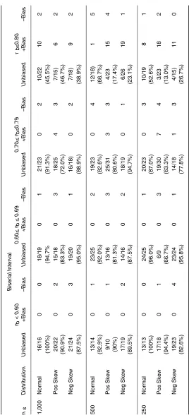
Table 2

Number of Biased and Unbiased Discrimination Estimates Categorized by the Biserial Correlation

Biserial Interval r b < 0.60 0.60 < r b < 0.69 0.70 < rb < 0. 79 rb < 0. 8 0

n s

Results Simulation Study

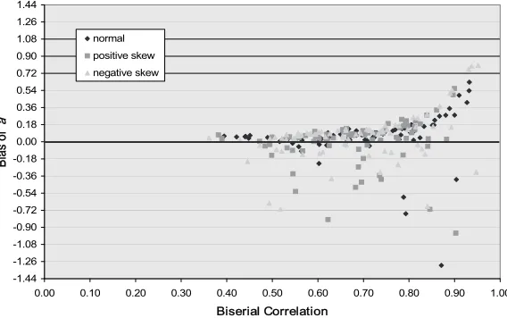
The simulation study examined the behavior of Lord’s formulas under condi-tions congruent and incongruent with the condicondi-tions prescribed by Lord. Al-though length of test was an independent variable, bias patterns were consistent across the 20-, 40-, and 80-item tests. Similarly, the bias patterns were consistent across the three sample sizes, although as expected, the standard errors increased as sample size decreased. Therefore, in the light of space limitations, the results for the 80 item tests with a sample size of 1,000 ex-aminees are presented graphically to illustrate the patterns of bias in the discrimination index and in the difficulty index (Figures 1, 2a, 2b).3 _{Bias is}

presented on the y-axis and the CTST index is provided on the x-axis. However, although the bias patterns were consistent across sample sizes, the numbers of unbiased and biased estimates for the three sample sizes are provided in accompanying tables given the importance of sample size in research and testing (Tables 2-4).

Item Discrimination

Lord’s formula for converting a CTST biserial correlation to the corresponding IRT discrimination is solely a function of the biserial correlation. Because IRT discrimination values typically range between 0 and 2 (Hambleton et al., 1991), mean standard errors were computed from the items within that range. The mean standard errors for the normal, positively skewed, and negatively skewed ability distributions were, rounded to two decimal places, 0.10, which suggests that estimates were fairly stable.

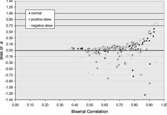
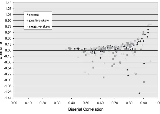
The bias patterns for the normal, positive, and negatively skewed ability distributions are illustrated as a function of the biserial correlation in Figure 1 for the sample size of 1,000 examinees. Items with discrimination estimates within of their true values were considered well estimated (a^_i = a_τ). Items above 0.20 possessed positive bias (a^i > aτ), while items –0.20 possessed nega-tive bias (a^i < aτ).

The numbers of well-estimated and positively and negatively biased item estimates are reported in Table 2 for four categories of the biserial correlation and the three sample sizes. The four biserial categories are based on values probably found in practice (e.g., r_b < 0.60 and 0.60 ≤ r_b ≤0.69) and the observa-tion that there were approximately equal numbers of items in each category.

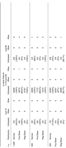
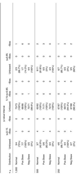
Table 3

Number of Biased and Unbiased Difficulty Estimates Categorized by p-value for the Equal Discrimination Condition

p -value Interval p < 0.15 0.15< p< 0.85 p < 0.85

n s

Lord’s formula for converting the CTST biserial correlation to the IRT discrimination did not work as well when the biserial correlation exceeded 0.69 and especially 0.79. Although the formula worked well for the three normal ability/sample size combinations and the negatively skewed distributions and two larger sample size combinations (at least 80% within two standard errors) for 0.70 ≤ rb ≤ 0.79, the formula worked less well for the remaining four combinations. When the biserial correlation was at least 0.80, no more than 67% of the estimates were within |0.20| of their true values. The largest bias occurred for biserial correlations close to one (e.g., when rb = 0.98, ar = 2.92, and

n=1,000, the bias was 4.22).

In summary, the results suggest that Lord’s formula for converting a biserial coefficient to the IRT discrimination index worked very well for items with biserial coefficients less than 0.70 regardless of the shape of the ability distribution and sample size and reasonably well for biserial correlations great-er than or equal to 0.70 and less than 0.80 and sample size of at least 500 examinees. However, the formula tends to overestimate when the biserial correlation is greater than or equal to 0.70 and less than 0.80 and the sample size is 250 examinees and when the biserial correlation was at least 0.80. Item Difficulty

Two conditions—equal discrimination and variable discrimination—were con-sidered when investigating the performance of Lord’s formula for converting the CTST difficulty index (p-value) to the corresponding IRT difficulty index (b-parameter). The numerator of this formula is the z-score associated with an item’s p-value. The z-score changes more rapidly as the two limits of the Figure 1. Bias of IRT discrimination estimates as a function of the CTST biserial correlation for the 80 item test, variable discrimination, and sample size of 1,000.

-1.44 -1.26 -1.08 -0.90 -0.72 -0.54 -0.36 -0.18 0.00 0.18 0.36 0.54 0.72 0.90 1.08 1.26 1.44

0.00 0.10 0.20 0.30 0.40 0.50 0.60 0.70 0.80 0.90 1.00

Biserial Correlation

Bias of

a

normal positive skew negative skew

Table 4

Number of Biased and Unbiased Difficulty Estimates Categorized by

p

-value for the Variable Discrimination Condition

p -value Interval p < 0.15 0.15<p< 0.85 p > 0.85

n s

p-value—0 and 1—are approached than when the p-values are moderate be-cause there are fewer examinees with extreme score values. The result is greater fluctuations from sample to sample within conditions, which serves to increase the variance error. Consequently, to avoid unrealistically high stan-dard errors, the mean variance errors of the estimated b-parameter estimates were computed from items with difficulties within the range 0.05 < p < 0.95. The mean standard errors for the normal, positive, and negatively skewed distributions for the condition of equal (unit) discrimination were 0.08, 0.10, and 0.11 and for the condition of variable discrimination were 0.08, 0.10, and 0.16 respectively. These values suggest that the estimated difficulties were fairly stable.

The results for the equal discrimination case, which was stipulated by Lord, are presented first. The results for the variable discrimination case follow.

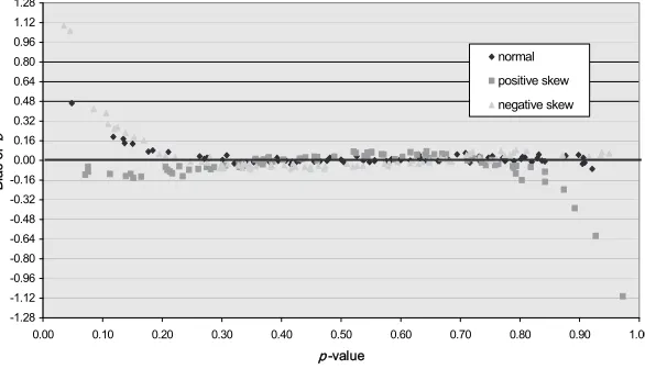
Equal discrimination. Lord (1980) stipulated that the discrimination be con-stant when using the formula for difficulty. The bias patterns for the normal, positive, and negatively skewed ability distributions are illustrated as a func-tion of the CTST difficulty in Figure 2a for the sample size of 1,000 examinees and equal item discrimination. Items with difficulty estimates within |0.20| of their true values were considered well estimated (b^i = bτ). Items above the upper limit of this interval possessed positive bias (b^i > bτ), while items below the lower limit of this interval possessed negative bias (b^i < bτ).

Figure 2a reveals that Lord’s formula for difficulty accurately predicted the true b-parameter for p-values between approximately 0.10 and 0.90 for the normal ability distribution. For items with the p-values less than 0.10, positive bias was observed; for items with p-values greater than 0.90, negative bias was observed. The distributions of bias for the positively and negatively skewed ability distributions were mirror images of each other. For the positively skewed ability distributions, the mean item b-parameters were well estimated for p-values between 0 and 0.85, but were underestimated for p-values greater than 0.85 (best fitting curve arced downward for the easier items). In contrast, for the negatively skewed distributions, the mean item b-parameters were well estimated for p-values between 0.15 and 1.00, but were overestimated for p-values less than 0.15 (best fitting curve arced upward for the most difficult items).

The numbers of well-estimated and positively and negatively biased item estimates are reported in Table 3 for three intervals of CTST difficulty and the three samples sizes. The limits of these difficulty intervals correspond to the breaks between unbiased and biased estimates of the b-parameter identified above. Figure 2a and Table 3 reveal that Lord’s formula for converting a p-value to the corresponding b-parameter worked well in the interval 0.15<p<0.85 regardless of the shape of the ability distribution. No fewer than 95% of the b-parameters were well estimated.

when ability was negatively distributed. In contrast, for p ≥ 0.85, the bias, although not as prevalent, was negative when ability was normally dis-tributed, negative for most of the items when ability was positively disdis-tributed, and absent for most of the items when ability was negatively distributed.

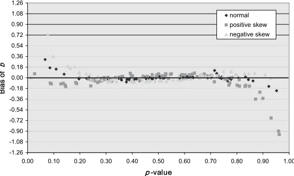
Variable discrimination. The presence of bias and the patterns of bias when converting p-values to b-parameter estimates using Lord’s formula but with variable rather than equal discrimination were consistent with the presence and patterns of bias observed with variable discrimination. As shown in Figure 2b and reported in Table 4, Lord’s formula for converting a p-value to the corresponding b-parameter worked well again in the interval 0.15 < p < 0.85 regardless of the shape of the ability distribution; for p ≤ 0.15, the bias was positive for approximately half of the items when ability was normally dis-tributed, absent for all the items when ability was positively disdis-tributed, and positive for all the items when ability was negatively distributed; and for p≥0.85, the bias, although not as prevalent, was negative when ability was normally distributed, negative for all the items when ability was positively distributed, and absent for all the items when ability was negatively dis-tributed.

Taken together, the results for unit and variable discrimination reveal that Lord’s formula for predicting b^i from pi and r′ix worked well for items with a broad range difficulties typically found in achievement tests (0.15 < p < 0.85). Item discrimination, whether constant or variable, had essentially no effect, which implies that the formula for converting p-values to b-parameter es-timates is robust. Without exception, when biases were observed, b^_i was over-estimated for difficult items (p ≤ 0.15) and underestimated for easy items

(p≥0.85). The bias patterns for the negatively and positively skewed ability

distributions were mirror images of each other: the easier items (p ≥ 0.85) were underestimated for the positively skewed ability distributions while the more Figure 2a. Bias of IRT difficulty estimates as a function of CTST item difficulty for the 80 item test, unit discrimination, and sample size of 1,000.

-1.28 -1.12 -0.96 -0.80 -0.64 -0.48 -0.32 -0.16 0.00 0.16 0.32 0.48 0.64 0.80 0.96 1.12 1.28

0.00 0.10 0.20 0.30 0.40 0.50 0.60 0.70 0.80 0.90 1.00

p -value

Bias

of

b

difficult items (p ≤ 0.15) were overestimated for the negatively skewed distribu-tions.

Achievement Data

Bias in the achievement data was calculated as the difference between Lord’s estimate and the BILOG (Mislevy & Bock, 1990, 2000) parameter estimate. The ability of Lord’s formulas to recover a- and b-parameters is considered with respect to both the biology and English exams. The analysis was replicated for 100 random samples of 1,000 examinees in order to calculate standard errors for the item parameters of the achievement data. The standard errors for the a-parameters were 0.06 for the biology exam and 0.05 for the English exam. The standard errors for the b-parameters were 0.15 for the biology exam and 0.14 for the English exam.

Because extreme bias values were not found with the achievement data, the presentation of bias for the two diploma examinations is in increments of one standard error in Figures 4 and 5. The CTST item indices appear on the horizontal axes, and the bias appears on the vertical axis. Further, because all the estimated a- and b-parameters were with five exceptions within two stan-dard errors, the results are presented in graphical form only.

Item Discrimination

As shown in Figure 3a, Lord’s formula for converting a biserial correlation to its corresponding a-parameter estimate worked well. All the a-parameter es-timates for both examinations were well estimated, being within |0.20| of their corresponding BILOG population values. Biases ranged between –0.035 and 0.081 for biology and between 0.016 and 0.080 for English.

Figure 2b. Bias of IRT difficulty estimates as a function of CTST item difficulty for the 80 item test, variable discrimination, and sample size of 1,000.

-1.26 -1.08 -0.90 -0.72 -0.54 -0.36 -0.18 0.00 0.18 0.36 0.54 0.72 0.90 1.08 1.26

0.00 0.10 0.20 0.30 0.40 0.50 0.60 0.70 0.80 0.90 1.00

p-value

Bias of

b

normal positive skew negative skew

Item Difficulty

Figure 3b displays the estimation bias of the difficulty parameter for the biol-ogy and English exams respectively in terms of item p-values. Again, Lord’s formula for converting a p-value to a b-parameter estimate worked well. All but two of the estimated b-parameters were within |0.20| of the corresponding BILOG population values for biology and all but six b-parameters for English. A common characteristic of the two biology items and the six English items, all of which exhibited positive bias, is that they possessed low biserial correla-tions, although it must be noted that not all items with low biserial correlations had biased b-parameter estimates.

Discussion

Several differences are seen between the present research and earlier studies that prevent direct comparison of the findings. First, the two-parameter IRT model was used for the present study, whereas the three-parameter model was used in the earlier studies. Second, the biserial correlation was used in the present study, whereas the point-biserial correlation was used in the earlier studies. Both these changes properly met the statistics identified by Lord (1980) when we first proposed the two formulas. The third difference is that the performances of Lord’s formulas were evaluated using different dependent variables. Estimation bias and sampling variances were calculated in the present study; correlational techniques were employed in the earlier studies. The fourth difference relates to the psychometric frame of reference. The es-timated IRT parameters were considered in relation to the classical item indices Figure 3a. Bias of IRT discrimination estimates as function of CTST biserial correlation for the English and biology exams.

-1.44 -1.26 -1.08 -0.90 -0.72 -0.54 -0.36 -0.18 0.00 0.18 0.36 0.54 0.72 0.90 1.08 1.26 1.44

0.00 0.10 0.20 0.30 0.40 0.50 0.60 0.70 0.80 0.90 1.00

Biserial Correlation

Bias of

a

normal positive skew negative skew

in the present study, whereas the IRT framework was used exclusively in the previous studies. Hence we discuss the results in the light of these differences. Item Discrimination

The results of the simulation study suggested that Lord’s formula for convert-ing the CTST biserial correlation to IRT item discrimination performed very well for biserial correlations of less than 0.70, and the results for the real achievement data confirmed this finding. Although the real achievement data represented a greater departure from normality than that modeled in the simulation study, the results were more similar to the data from the normal ability distribution where all items with biserial coefficients less than 0.70 were well estimated. Another difference between the simulated and real achieve-ment data was the kurtosis of the ability distributions. The IRT ability distribu-tions of the two achievement data sets were leptokurtic, whereas the skewed ability distributions in the simulation study were platykurtic. Therefore, it appears that Lord’s discrimination formula is robust to the violation of the assumption of a normal ability distribution when the biserial coefficients are less than 0.70.

These findings are not consistent with the opinions put forth by Schmidt (1977). In the context of Urry’s (1974) graphical procedure that used the point-biserial correlation and the three-parameter IRT model, Schmidt proposed that a

^

i would be systematically underestimated. He reasoned that the point-biserial correlation between the item score and the estimated latent trait (i.e., total test score), r_iθ^ , is taken as an estimate of the point-biserial correlation between the item score and the perfectly reliable latent trait, ρ^iθ. Values of riθ^ will be attenuated because of guessing on item i, and the unreliability of θ^. Schmidt pointed out that increased values of the correlation would lead to larger a^i. No subsequent work has verified this criticism of Urry’s research. However, the Figure 3b. Bias of IRT difficulty estimates as a function of CTST item difficulty for the English and biology exams.

-1.44 -1.26 -1.08 -0.90 -0.72 -0.54 -0.36 -0.18 0.00 0.18 0.36 0.54 0.72 0.90 1.08 1.26 1.44

0.00 0.10 0.20 0.30 0.40 0.50 0.60 0.70 0.80 0.90 1.00

Biserial Correlation

Bias of

a

normal positive skew negative skew

results of the present study suggest that the discrimination parameters were not systematically underestimated. Rather, they were well estimated in the context Lord intended: using the biserial correlation and the two-parameter IRT model.

Item Difficulty

Schmidt (1977) contended that |b^_i| derived from Lord’s formula for convert-ing CTST p-values to IRT b-parameter estimates would be systematically over-estimated in the context of Urry’s (1974) work. Results from the present study suggest that this is not the case when the biserial correlation and the two-para-meter IRT model are used. The results of the simulation study suggested that Lord’s formula for item difficulty performed quite well for p-values between 0.15 and 0.85, regardless of the shape of the ability distribution. The patterns of bias in the b-estimates observed for the conditions of variable discrimination were comparable to the patterns of bias in the b-estimates observed for unit discrimination. Seemingly, Lord’s restrictions of equal item discrimination and normal ability distribution are not required for a broad range of difficulty values (i.e., 0.15 < p < 0.85).

When biased difficulty estimates occurred, they were differentially affected by the direction of the skewness. Bias was most pronounced and negative for the easy items in the positively skewed distribution and most pronounced and positive for the difficult items in the negatively skewed distribution. These results may be explained by examining the nature of the skewed distributions. Fewer examinee ability values were observed in the non-tailed region than the tailed region. There were few ability values at the high end of the ability scale (θ > 2.20) for the negatively skewed population and there were few ability values at the low end of the ability scale (θ < –2.20) for the positively skewed population. The result is floor and ceiling effects respectively. The effect on b-parameter estimation is dramatic. The numerator of the formula is a z-score, which changes more rapidly as p-values reach very high and very low levels, driving up the absolute value of the z-score. As a consequence, bi is overes-timated when most examinees answer incorrectly and bi is underestimated when most examinees answer correctly. Although high p-values (i.e., p > 0.85) and low p-values (i.e., p < 0.15) are not desirable item characteristics, the findings highlight the limitation of the formula to predict IRT difficulty para-meters accurately in such circumstances.

possible explanation is related to the violation of the assumption of non-guess-ing. Hambleton et al. (1991) stated that the assumption of no guessing is most plausible with constructed-response items, but may be met only approximately with multiple-choice items when a test is not too difficult for the examinees. For example, they suggested that this assumption might not be met when tests are given to students following effective instruction.

A second reason why the assumption of guessing may have been only partly met is the presence of items susceptible to the application of testwise-ness. Review of the item content, including the item options, revealed that the five items were susceptible to testwiseness. Testwiseness has been defined as a person’s ability to use the characteristics and formats of the test and/or the test-taking situation to improve his or her test score. If an examinee possesses relevant partial knowledge of the content area and knowledge of testwiseness strategies, and if the test contains testwise-susceptible items, then the combina-tion of these elements may result in a higher test score (Rogers & Bateson, 1991). Examinees may eliminate incorrect options and select among the remaining choices, thereby increasing their chances of success on these items. Consequently, the five biased items exhibited low biserial correlations. As Lord and Novick (1968) pointed out, this is what is expected from items that can be answered correctly by guessing because the item score cannot be highly corre-lated with any criterion. A low biserial correlation would contribute to the overestimation of bi, given the biserial is the denominator of the formula for converting p-values to b-parameter estimates.

classical test score p-value to the corresponding b-parameter estimate. To echo the sentiments of Jensema (1976), Lord’s formulas yield “surprisingly accurate” estimates of IRT discrimination and difficulty.

Notes

1_{The observation that the classical and IRT distributions have opposite directions of skewness is}

attributable to the difference in way the difficulty parameter is defined in the two test models. Low p-values reflect difficult items whereas negative b-values reflect difficult items.

2_{Use of a conceptually reasonable value was adopted instead of using standard errors and}

confidence intervals so as to provide an overall fit criterion rather than one that varied by item difficulty and/item discrimination.

3

The results for the 20 and 40 item tests and sample sizes 250 and 500 for the 80 item test can be obtained from the first author.

References

Alberta Education. (1999). Alberta Education annual report 1998-1999. Edmonton, AB: Author. Alberta Learning. (1999a). Biology 30 grade 12 diploma examination, June 1999. Edmonton, AB:

Author.

Alberta Learning. (1999b). English 30 grade 12 diploma examination, June 1999. Edmonton, AB: Author.

Fan, X. (1998). Item response theory and classical test theory: An empirical comparison of their item/person statistics. Educational and Psychological Measurement, 58, 357-381.

Gifford, J.A., & Swaminathan, H. (1990). Bias and the effect of priors in Bayesian estimation of parameters of item response models. Applied Psychological Measurement, 14, 33-43.

Hambleton, R.K. (1989). Principles and selected applications of item response theory. In R. Linn (Ed.), Educational measurement (3rd ed., pp. 147-200). New York: Macmillan.

Hambleton, R.K., Swaminathan, H., & Rogers, H.J. (1991). Fundamentals of item response theory. Newbury Park, CA: Sage.

Harwell, M., Stone, C.A., Hsu, T., & Kirisci, L. (1996). Monte Carlo studies in item response theory. Applied Psychological Measurement, 20, 101-125.

Jensema, C. (1976). A simple technique for estimating latent trait mental test parameters.

Educational and Psychological Measurement, 36, 705-715.

Lord, F.M. (1980). Applications of item response theory to practical testing problems. Englewood Cliffs, NJ: Erlbaum.

Lord, F.M., & Novick, M.R. (1968). Statistical theories of mental test scores. Reading, MA: Addison-Wesley.

MacDonald, P., & Paunonen, S.V. (2002). A Monte Carlo comparison of item and person statistics based on item response theory versus classical test theory. Educational and Psychological Measurement, 62, 921-943.

Mislevy, R.J., & Bock, R.D. (1990). BILOG 3: Item analysis and test scoring with binary logistic models

(2nd ed.). Mooresville, IN: Scientific Software.

Mislevy, R.J., & Bock, R.D. (2000). BILOG 3.2: Item analysis and test scoring with binary logistic models [Computer program]. Mooresville, IN: Scientific Software.

Nandakumar, R. (1994). Assessing dimensionality of a set of item responses—Comparison of different approaches. Journal of Educational Measurement, 31, 17-35.

Nelson, L.R. (2000). Laboratory of education research test analysis package (LERTAP, Version 5) [Computer program]. Perth, W. Australia: Curtin University of Technology.

Nelson, L.R. (2001). Item analysis for tests and surveys using LERTAP 5. Perth, W. Australia: Curtin University of Technology.

Ree, M.J. (1979). Estimating item characteristic curves. Applied Psychological Measurement, 3, 371-385.

Rogers, W.T., & Bateson, D.J. (1991). The influence of test-wiseness upon the performance of high school seniors on school leaving examinations. Applied Measurement in Education, 4(2), 159-183. Schmidt, F.L. (1977). The Urry method of approximating the item parameters of latent trait

theory. Educational and Psychological Measurement, 37, 613-620.

Spearman, C. (1904). The proof and measurement of association between two things. American Journal of Psychology, 15, 72-101.

Stage, C. (1998a). A comparison between item analysis based on item response theory and classical test rheory. A study of the SweSAT subtest ERC. (Educational Measurement No. 30). Umea, Sweden: University of Umea, Department of Educational Measurement.

Stage, C. (1998b). A comparison between item analyses based on item response theory and on classical test theory. A study of the SweSAT subtest WORD. (Educational Measurement No. 29). Umea, Sweden: University of Umea, Department of Educational Measurement.

Stage, C. (1999). A comparison between item analysis based on item response theory and classical test theory. A study of the SweSAT subtest READ. (Educational Measurement No. 33). Umea, Sweden: University of Umea, Department of Educational Measurement.

Traub, R.E. (1983). A priori considerations in choosing an item response model. In R.K. Hambleton (Ed.), Applications of item response theory (pp. 57-70). Vancouver, BC: Educational Research Institute of British Columbia.

Urry, V.W. (1974). Approximations to item parameters of mental test models and their uses.

Educational and Psychological Measurement, 34, 253-269.

Wolfram, S. (2000). Mathematica for students (Version 4) [Computer program]. Wolfram Research. Yen, W.M. (1987). A comparison of the efficiency and accuracy of BILOG and LOGIST.