556 Abstract—In this paper a method based on the Particle Swarm Optimization (PSO) algorithm is presented for tuning Power System Stabilizer (PSS) parameters. In the proposed method, based on the optimization of a suitable objective function, optimal values for PSS controlling parameters including lead-lag compensator time constants as well as the controller gain are calculated. The employed objective function is the damping ratio of eigenvalues corresponding to system critical modes obtained from the analysis of the linearized model of system around the operating point. Controllable and critical modes of the system are identified using modal controllability and observability criteria. The proposed algorithm is applied to a single machine power system and for various operating conditions. Simulation results prove the capability of the proposed algorithm in damping improvement of power system.
Index Terms— controllability, observability, particle swarm optimization, power system stabilizer, root locus.
I. INTRODUCTION
A power system is consisted of generators, loads, transformers, and transmission lines. A disturbance in the power system will cause electromechanical oscillations and hence, system variables will start to oscillate. These variables may include system voltage, frequency, load angles of generators, or other parameters of the system. Stabilizing these parameters is of great importance in power system stability [1]. Controllers designed with classic methods, despite their simplicity, are only suitable for specific operating conditions of the system and will not work for many unpredicted situations [2-4]. Therefore, when the operating point of the system varies, oscillations may not be damped satisfactorily and even the system may become unstable. This is due to the fact that parameters setting of the controller which is suitable for a point of system operating condition will not be satisfactory for other points. Although adaptive control methods eliminate this drawback to a great extent [5], they are rather complex and costly. Thus, the necessity for designing a simple controller that can make the system stable against the disturbances in a wide range of operating conditions will be of great value. Once the structure of controller is specified, it can be said that the method for parameter setting is not that much important since
Manuscript received August 18, 2010.
A. Jalilvand is with the Electrical Engineering Department, Zanjan University, Zanjan, Iran (phone: +98-241-5152610; fax: +98-241-2283204; e-mail: ajalilvand@ znu.ac.ir).
M. Daviran Keshavarzi., was with the Electrical Engineering Department, Zanjan University, Zanjan, Iran (e-mail: [email protected]).
an accurate design means the accurate setting of parameters. In applications in which a simple, fast, and a suitable setting for at least several points of system operating conditions are needed, the effectiveness of classic methods may be restricted. Optimization methods which are based on random search algorithms are very suitable for solving complex problems that are difficult or even impossible to be solved using conventional mathematical methods such as gradient [6]. Power system stability is one of these problems as solving differential equations of power system in order to investigate its stability is an intricate problem. Application of such methods in solving complicated problems has recently been in the focus of researchers' attention [7-9]. For instance, in [9] the multi-objective Genetic algorithm has been utilized for tuning the controller parameters. In some applications, the steady state error of system factors, which cause the system to become stable, is minimized by the algorithm [10].
The paper is organized as follows: in Section II, linear model of a power system is explained and discussed along with mathematical equations. In Section III, modal analysis is explained. Next, controllability and observability concepts are briefly reviewed in Section VI. Particle Swarm Optimization is studied in Section V and the objective function is presented and explained in Section VI. Next, the proposed algorithm is applied to the considered system and simulation results are discussed in Section VII. Finally, conclusions are presented in Section VIII.
II. LINEAR MODEL OF APOWER SYSTEM
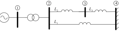
In this paper, a power system consisted of a single machine connected to the infinite bus (SMIB) is considered where its parameters and single line diagram are presented in the Appendix and Fig. 1, respectively.
L2
L1
L3
1
2 3 4
Fig. 1. Single machine power system connected to the infinite bus
The third order model is considered for the generator that includes two differential equations for rotor electro-mechanic oscillations and one equation representing the internal voltage of generator [11, 12].
) 1 ( − =ω ω
δ b (1)
PSO Algorithm-Based Optimal Tuning of PSS
for Damping Improvement of Power Systems
557
( ( 1))
1
− − −
= ω
ω P P D
M m e
(2)
(
Fd d d d q)
do
q T E x x i E
E − − ′ −
′ =
′ 1 ( )
(3)
In the above-mentioned equations, δ and ω are mechanical degree and rotor speed, respectively; ωb is the reference speed;
M is the rotor inertia constant; D is the rotor friction constant; Pe and Pm are electrical output power and mechanical input
power, respectively; Eq is the internal voltage of the machine;
Efd is the exciting voltage; τ'do is the time constant of open
circuit excitation; Xd and X'd are the steady state and transient
reactances of the machine on d axis, respectively; and id is the
stator current along d axis.
The relationship between output electrical power and the machine voltages and currents is as follows:
q q d d
e v i v i
P = + (4)
Where vd, vq, id, and iq are voltage and current components of
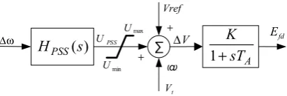
the machine along d and q axes, respectively, and are obtained using the initial conditions of the system. The IEEE-ST1 generator with excitation system and self-controlled voltage together with PSS is shown in Fig. 2.
Vref
t
V
V
Δ Efd
Umax
Umin UPSS
Δω +
+
@ sTA
K + 1 )
(s HPSS
Fig. 2. IEEE-ST1 excitation system together with PSS.
In this system, the voltage excitation system is as follows:
] ) (
[ 1
fd PSS t erf A A
Fd K v v u E
T
E′ = − + −
(5)
Where Vt and Vref are terminal voltage and reference voltage,
respectively; upss is the stabilizer signal; and KA as well as TA
are transient state gain and excitation time constant, respectively. Moreover, the equations of voltages are:
2 2
q d
t v v
v = + (6)
q q
d x i
v = (7)
d d q
q E x i
v = ′− ′ (8)
The classic model of the power system PSS controller includes two lead-lag compensating blocks as well as a filter and a gain [8-11].
⎟⎟ ⎠ ⎞ ⎜⎜
⎝ ⎛
+ + ⎟⎟ ⎠ ⎞ ⎜⎜
⎝ ⎛
+ + ⎟⎟ ⎠ ⎞ ⎜⎜
⎝ ⎛
+ =
Δ Δ =
4 3
2 1
1 1 1
1 1
) (
sT sT sT
sT sT
T K
U s H
W w PSS PSS
PSS ω (9)
Where T1, T2, T3, and T4 are lag compensator time constants; Tw is the filter time constant; and Kpss is the
constant gain of the controller. Tw is selected large enough so
that only the variations are permitted to pass.
III. MODEL ANALYSIS
The linearized model of system in the state space is utilized to identify the oscillatory modes and to set the PSS parameters. The equations of the linearized model in the state space are given by [11]:
u B x A x= Δ + Δ
Δ (10)
Where Δx is the column vector of state variables with the degree of n; A and B are state and input matrixes with consistent dimensions, respectively; and Δu is the input vector with the length of r.
In this system, the state variables and input vectors are as follows:
[
]
[
m ref]
T
fd q
v P u
E E x
Δ Δ = Δ
Δ ′ Δ Δ Δ =
Δ δ ω
(11)
Various methods may be employed to linearize the system. The linearization of equations (1) to (8) in order to get to equation (10) is described thoroughly in [11, 12]. Here, it is assumed that the system is linearized around the operating point and the state space realization is available. The system eigenvalues are obtained using the characteristic equation of matrix A and from (12):
0 )
det(λI−A = (12)
There exists a column eigenvector φi for each individual
eigenvalue λi satisfying the following equation:
i i i
Aφ =λφ (13)
Where φi is the right eigenvector corresponding to the
eigenvalue λi; and in the similar way, the left eigenvector ψi
corresponding to the eigenvalue λi is given by:
i i iA λψ
ψ = (14)
Modal matrixes are obtained employing right and left eigenvectors.
] [
] [
2 1
2 1
T n T
T
n
ψ ψ
ψ
φ φ
φ
" " =
Ψ = Φ
(15)
558 oscillatory mode. A left eigenvector includes information about the controllability of modes. For each complex eigenvalue λi=σi±jωi , damping ratio in percent is defined as follows:
2 2
i i
i i
ω σ
σ ξ
+ −
= (16)
The modes having less than 3% damping ratio are known as critical modes [11] and the controller should be designed in a way that their damping ratio is improved by changing the locations of these eigenvalues. However, considering a certainty margin is necessary due to uncertainties and disturbances. Hence, the damping ratio less than 5% is considered in designing and the PSO algorithm is employed in this paper to obtain this goal.
IV. CONTROLLABILITY AND OBSERVABILITY
In order to control an oscillatory mode using a suitable feedback, the controller output should have impact on that mode and on the other hand, that mode should be observable in that feedback. The behavior of the oscillatory mode is mirrored in the feedback signal. In order to investigate this case, the controllability and observability criteria are employed whose matrixes are defined as follows [11]:
Φ =
Φ = −
C C
B B
m m
1
(17)
If the corresponding row of a mode in Bm is zero, that
mode will not be controllable and if the corresponding column of a mode in Cm is zero, that mode will not be
observable. If a mode is not controllable and observable, the feedback between input and output will not have any effects on it [14].
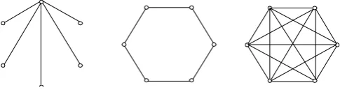
V. PARTICLE SWARM OPTIMIZATION ALGORITHM Particle Swarm Optimization (PSO) is a population based stochastic optimization technique developed by Dr. Kennedy and Dr. Eberhart in 1995, inspired by social behavior of bird flocking or fish schooling [6, 15, and 16]. It is based on exchanging information among the particles in a network. In general, three topologies can be considered for the particles in a network known as star, ring, and rotiform topologies. Theirs structures are presented in Fig. 3
Fig. 3. The topologies utilized in the PSO algorithm.
In the star topology each particle is able to associate with all of the particles in the swarm and each particle wants to
follow the population best movement. In the ring topology, each particle associate with its n neighboring particles and wants to follow the movement of the best neighboring particle. In the rotiform topology, all of the particles relate with a particle called canonical particle. This topology is based on traveling geese which obey their leader.
Based on the three above-mentioned topologies for particles, Global best, Individual best, and Local best algorithms can be considered for optimizations which employ star, ring, and rotiform topologies, respectively.
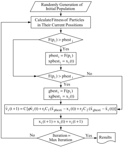
Global best and Local best algorithms are the most common ones for optimizations. The former intends to search in vast areas and the latter intends to search in small areas and existing points in the neighborhood. These two algorithms are structurally similar to each other and they are sometimes used in a mixed form. In this paper, the Global best algorithm is employed to solve the optimization problem. In this algorithm, a population consisting of L individuals from X vectors is considered. The X vector has n particles each referred as a PSS unknown variable. First, the swarm is randomly given values and next, the particles are steered towards the objective, i.e., finding the minimum point. The position of each particle is its corresponding X vector with the value of the fitness function in the associated position. During the algorithm process, the best experience of each particle and its corresponding position can be saved. The best experience of the ith particle is called pbest
i and its
corresponding position is known asxGpbesti
.
In a similar way, the best experience existing among all of the particles and their corresponding positions are called gbestiandxGgbesti, respectively.In moving towards the minimum point, the velocity of each particle and its updated position is identified by (18) and (19), respectively.
))] ( (
2 2
)) ( (
1 1 ) ( [ ) 1 (
t i x i gbest x C r
t i x i pbest x C r t i v C t i v
G G
G G
G G
− +
− +
=
+ ϕ
(18)
) 1 ( ) ( ) 1
(t+ =x t +v t+
xi i i
G G G
(19)
Where:
) (t
vGi : The current velocity of ith particle;
) 1 (t+
vGi : The next velocity of ith particle;
φ: inertia weight; r1: cognitive factor;
r2:social factor;
C: contraction factor;
C1 and C2: acceleration constants.
559 i
i) pbest
F(p >
(t) x xpbesti= i
i i) pbest
F(p >
) F(p gbesti= i
(t))] x x ( C r (t)) x x ( C r (t) ν [ C 1) (t
νi Gi 1 1Gpbesti i 2 2 Ggbesti Gi G
− +
− +
=
+ ϕ
1) (t ν (t) x 1) (t
xi + = i + i +
Yes
No
Yes
No Yes
Particles of Fitness Calculate
Possitions Current Their in
of Generation Randomly
Population Initial
Results
=
Iteration Iteration Max
(t) x xgbesti= i
) F(p pbesti= i
Fig. 4. Flow chart of the PSO algorithm.
A change in these parameters will affect the algorithm sensitivity and accuracy to a great deal. The values for the above-mentioned parameters are all experimental and there is not theoretical method for their accurate calculation. Considering an upper bound for the velocity will cause the particles not to jump with a high velocity in the search area and thus, the space is more accurately assessed in order to find more desirable areas and furthermore, the algorithm divergence due to high velocities is prevented. When the velocity vector of each particle is updated, the following constraint is applied:
max max
max max
) ( )
( :
) ( )
( :
V t V V t V if
V t V V t V if
i i
i i
− =
⇒
<
=
⇒
>
(20)
The contraction factor controls the effect of velocity in updating the particles positions considering the parameters limits. The inertia weight controls the effect of previous velocity on the current velocity. Large values of this parameter will cause a larger search in the search space and its smaller values will lead in focusing on a smaller area. r1
and r2 are random numbers in the range (0, 1) and C1 as well
as C2 are positive numbers. Due to a study on the effect of C1
and C2 on the particles movement paths, the following
constraint is proposed as a necessary condition for the algorithm convergence:
4
2 1+C ≤
C (21)
VI. OBJECTIVE FUNCTION
Selecting the objective function is the main part of the PSO algorithm. The purpose of the algorithm is to improve the stability as well as damping improvement of the power system. Any function that can achieve this goal may be selected as the fitness function. In some researches the steady state error of those system factors in which oscillation
damping will lead in system stability are utilized [10]. These factors, depending on the controller type, may be the active power flow from the transmission line, bus voltage or current or relative speed of the generator. Indeed, the main goal is to increase the damping ratio of oscillatory and controllable modes in the system. Every setting which can achieve this goal can optimize the power system stability. On the other hand, the PSO algorithm is able to find this solution by searching in a space that is defined for parameters. Hence, maximizing the damping ratio of critical oscillatory modes
%) 5
(ξ< is selected as the objective function which is defined
as follows:
) ( min max ξ
n p
J =
(21)
Subject to:
max , 4 4 min , 4
max , 3 3 min , 3
max , 2 2 min , 2
max , 1 1 min , 1
max , min
,
T T T
T T T
T T T
T T T
K K
KPSS PSS PSS
≤ ≤
≤ ≤
≤ ≤
≤ ≤
≤ ≤
(22)
In the above equations, p is the number of selected operating points and n is the number of eigenvalues with a relative damping less than 5%. In the optimization stage several operating points of the system can be utilized so that the controller would work suitably over a wide range of operating conditions. Equation (23) expresses the selected ranges of controlling parameters. The suitable selection of these ranges is of great importance in getting to an optimal setting. In order to specify the permitted ranges, the root locus method can be applied.
VII. SIMULATION RESULTS AND DISCUSSION The proposed algorithm is applied to the presented system in Fig. 1 and the PSS parameters are calculated. In order to get an accurate result as well as a fast convergence of the algorithm, the values of the aforementioned parameters are considered as summarized in Table (1).
TABLEITHE VALUES OF PSO PARAMETERS
Dimension 5
Number of particles 50
Number of iterations 50
Maximum velocity 1
Inertia weight 0.75
r1 A random number in the range (0 , 1)
r2 A random number in the range (0 , 1)
C1 1.7
C2 1..9
C 0.6
560 cause the system operating conditions to change for linearization. Generally, the more the number of such points, the more the validity of obtained results.
The uncontrolled system has a critical mode with a damping less than 5% as shown in Fig. 5.
-2 -1.5 -1 -0.5 0 0.5
0 2 4 6 8 10 12
σ
j
ω Critical mode
Damping ratio=5%
Fig. 5. Eigenvalues locus of the uncontrolled system.
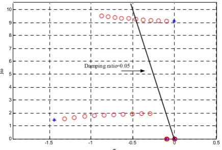
The root locus presents a suitable criterion to know the approximate ranges of the PSS parameters. For example, Fig. 6 shows the movement of system eigenvalues for the variation of constant gain KPSS from zero to 30.
-1.5 -1 -0.5 0 0.5
0 1 2 3 4 5 6 7 8 9 10
σ
j
ω Damping ratio=0.05
Fig. 6. System root locus for KPSS variations from zero (*) to 30 (○).
Applying the algorithm to the considered system, the parameters of the PSS transfer function are calculated. The results are summarized in Table (2).
TABLEIICALCULATED PARAMETERS USING THE PSO ALGORITHM
KPSS TW T1 T2 T3 T4
9.87 10 0.013 0.022 2.888 2.152
The algorithm performance is in a way that when the minimum damping ratio gets the desirable value(ξ ≥0.05)
in the maximum iteration, the algorithm will stop. Fig. 7 depicts the closed loop eigenvalues of this system compared to the conventional method setting as well as uncontrolled system.
The validity of the PSO-based setting is completely clear from Fig. 7. The noticeable point in Fig. 7 is the second eigenvalue which not only has not moved to the positive side of the real axis, but also it has moved to the negative side of the axis.
-3.5 -3 -2.5 -2 -1.5 -1 -0.5 0
0 2 4 6 8 10 12
σ
j
ω
Base Case Conventional Tuning PSO Tuning
Damping ratio=5%
Fig. 7. Closed loop eigenvalues movement with PSO setting (□) compared to conventional method setting (○).
As mentioned before, stochastic searching algorithms are able to search in a defined space and find the optimum points. Fig. 8 shows the algorithm convergence for the considered objective function. In general, the accuracy and convergence ratio of the PSO algorithm is more than other optimization algorithms as it is observed in Fig. 8.
0 5 10 15 20 25 30 35 40 45 50
0.52 0.54 0.56 0.58 0.6 0.62 0.64 0.66
Iterations
J
Fig. 8. The PSO convergence based on the objective function.
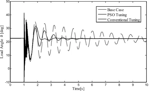
In order to better assess the capabilities of the designed stabilizer, time-based simulation of the system is utilized under disturbance. In the first step, a high amplitude disturbance is considered, which is a three-phase fault occurred in t=1s on the bus 3 with a duration of 10 cycles. After two cycles, lines L2 and L3 are disconnected from two ends. Figs. 9 and 10 show the machine speed oscillations based on the reference speed in pu and its load angle in degrees, respectively.
0 1 2 3 4 5 6 7 8 9 10
-0.015 -0.01 -0.005 0 0.005 0.01 0.015
Time[s]
R
ot
or
S
pee
d D
ev
iat
io
n
Δω
[p
u]
Base Case PSO Tuning Conventional Tuning
561
0 1 2 3 4 5 6 7 8 9 10
-10 0 10 20 30 40 50 Time[s] L oad A ng le δ [d eg ] Base Case PSO Tuning Conventional Tuning
Fig. 10. The machine load angle in degrees for a three-phase fault in bus 3.
In the previous step, the input mechanical power of the generator was assumed to be constant. In the second stage the system is affected by a step disturbance in the input mechanical power and it is simulated considering a 20% increase in the mechanical power in t=1s for 500 ms.
Figs. 11 and 12 depict the rotor speed deviation and output electrical power of the generator, respectively. The results of this stage reveal that the PSO setting for this type of disturbance does not differ a lot with the conventional setting method.
0 1 2 3 4 5 6 7 8 9 10
-4 -3 -2 -1 0 1 2 3x 10
-3 Time[s] R ot or S pee d D ev iat io n
Δω [p
u]
Base Case PSO Tuning Conventional Tuning
Fig. 11. The generator speed deviation for a step increase in the mechanical input power.
19 20 21 22 23 24 25 26 27 28 29
0.7 0.8 0.9 1 1.1 1.2 1.3 1.4 Time[s] O utp ut E le ctr ic al P ow er [p u] Base Case PSO Tuning Conventional Tuning
Fig. 12. The generator output active power oscillations for a step increase in the mechanical input power.
VIII. CONCLUSION
In this paper, tuning of Power System Stabilizer (PSS)
parameters is studied for a single machine system by means of PSO algorithm. The objective function is defined based on the system linear model analysis around the operating point and the objective is to find the critical oscillatory and controllable modes and next, to increase their damping. The algorithm criteria in order to find these modes are controllability and modal observability matrixes as well as a damping ratio less than 5%. As the algorithm is employed for various operating conditions, the obtained results will be valid for a vast range of operating conditions. Comparing the simulation results of the proposed algorithm with those of a conventional-tuned controller reveal that the PSO-based setting works better even for high amplitude disturbances such as short circuits.
APPENDIX
All of the parameters as well as values of initial conditions for system simulation are in pu otherwise it will be mentioned. MVA Kv Q P Hz f r T T s T X X X Xq X D s H e e s q do do q d d d 200 8 . 13 : Values Rated 23 , 35 . 0 , 875 . 0 60 , 003 . 0 0513 . 0 0681 . 0 , 49 . 4 243 . 0 252 . 0 , 296 . 0 , 474 . 0 305 . 1 , 0 , 7 . 3 : Genarator o 0= = = = = = ′′ = ′′ = ′ = ′′ = ′′ = ′ = = = = δ 02 . 0 , 100 :
Exciter KA= TA=
MVA S KV V V j X j X bsee base L L L 200 230 0 997 . 0 0567 . 0 , 1134 . 0 : Line on Transmissi 4 3 , 2 1 = = ∠ = = = D 08 . 0 0027 . 0 : r
Transforme + j
4 . 5 , 3 , 02 . 0 05 . 0 , 10 , 10 : PSS al Convention 4 3 2 1 = = = = = = T T T T T
KPSS w
REFERENCES
[1] A. D. DelRosso, C. A. Canizares and V. M. Dona, “A Study of TCSC Controller Design for Power System Stability Improvement,” "Influence of harmonics on power distribution system protection," IEEE Trans. Power System, vol. 18, no.4, Nov. 2003.
[2] A. D. DelRosso, C. A. Canizares and V. M. Dona, “A Study of TCSC Controller Design for Power System Stability Improvement,” IEEE Trans. Power System, vol. 18, no.4, Nov. 2003.
[3] C. Y. Chung, K. W. Wang, C. T. Tse, and R. Niu, “ Power System Stabilizer (PSS) Designe by Probabilistic Sensitivity Indexes(PSIs), ” IEEE Trans. Power System, vol. 17, no.3, Aug. 2002.
[4] N,Yang,Q.Liu,J.D,MacCalley, “ TCSC Controller Designe for Damping Interarea Oscillations, ” IEEE Trans. Power System, vol. 13, no.4, Nov. 1998.
[5] Wenyan. Gu, “System damping improvement using adaptive power system stabilizer, ” in Proc 2004 IEEE Canadian Conference on Electrical and Computer Engineering, pp. 1245-1247.
[6] Randy L. Haupt, Sue Ellen Haupt, “Practical Genetic Algorithms,” 2nd Edition, John Willy & Sons Inc., 2004.
[7] M. Dubey and A. Dubey, “Simultaneous Stabilization of Multi-machine Power System Using Genetic Algorithm Based Power System Stabilizers,” in Proc. 2006 41st International IEEE Power Engineering Conf., pp. 426-431.
562 [9] Y. L. Abdel-Magid, “Optimal multi-objective design of robust power
system stabilizers using genetic algorithms, ” IEEE Trans. Power System, vol. 18, no.13, pp. 1125-1132, Aug. 2003.
[10] M. A. Abido, “Design of PSS and STATCOM-based damping stabilizers using genetic algorithms, ” presented at the IEEE Power Engineering Society General Meeting, 2006.
[11] P.Kundur, “Power System Stability and Control," McGraw Hill, New York, 1994.
[12] P.M.Anderson and A.A.Fouad, “Power System Control and Stability, ” IEEE Press, 1994.
[13] IEEE Recommended Practice for Excitation System Models for Power System Stability Studies, IEEE Standard 421.5-1992.
[14] R. K. Sadikovic, and P.Andersson, “ Application of FACTS devices for damping of power system oscillations, ” in Proc 2005 IEEE Power Tech. Conference, Russia, pp. 1245-1247.
[15] M.Clerc, “Particle Swarm Optimization, ” ISTE Ltd., New Port Beach, CA, 2006.
[16] X. F. Xie, W. J. Zhang, and Z. L. Yang, “ A Dissipative Particle Swarm Optimization, ” in Proc 2002 Congress on Evolutionary Computation, Hawaii, USA, pp. 1456-1461, 2002.
Abolfazl Jalilvand was born in Taketan, Iran, 1972. He received B. Sc. in Electrical and Electronic Engineering from Electrical and Computer Engineering Faculty of Shahid Beheshti University, Iran, in 1995. He received M. Sc. and PhD degrees from Electrical and Computer Engineering faculty of Tabriz University, Iran, in Power Engineering and Control Engineering in 1998 and 2005, respectively.
In 2006 he joined the Electrical Engineering Department of Zanjan University, Iran, as an assistant professor where he is dean of faculty now. His main research interests include the Hybrid Control Systems, Petri Nets, Intelligent Control, Modeling and Control of Power Electronic Converters, Control and Stabilization of Power Systems, Application of Intelligent methods in Power Systems and so on. He has over 65 papers in journals and conferences.
Dr Jalilvand is a member of the Institute of Electrical and Electronic Engineers (IEEE). Also he is a senior member of International Association of Computer Science and Information Technology (IACSIT).
Morteza Daviran Keshavarzi was born in Tehran, Iran, 1982. He received B. Sc. in Electrical Engineering from Engineering Faculty of Islamic Azad University, Tehran South Branch, Iran, in 2005. He received M. Sc. degree from Engineering Faculty of Zanjan University, Iran, in Power Engineering in 2008.