implemented in the hybrid system on the site of Laboratory of Research Applied to Renewable Energy (LRAER). It gives also, estimation and evaluation of the production which encompasses performance of the energy conversion system of a wind turbine. To analyze the influence of the interference factor on energy production, our simulations are realized in Matlab environment. The results of this work provide a previous estimation about the suitability between the specific wind turbine type and the installation site.
Index Term-- Wind turbine, Bornay 3000, efficiency, Axial force, Hybrid system.
1. INTRODUCTION
Today, renewable energies have become a focus for the world, given that they are clean and sustainable. This interest is encouraged through wholesale funding for the scientific research in this field. In general, the place of proliferation for longer wind turbines corresponds to coastal areas. Within this framework, the zones of the Atlantic littoral Mauritanian, this has over six hundred kilometers of potential use for wind energy.
In this paper, we present
an approach of calculation of the blades for the aerogenerator, which has two blades with a horizontal axis. The developed mathematical models are based on the Betz theory, this method is used to extract the maximum power of energy within the wind speed’s intervals. They are recorded on LRAER or Bornay3000, which corresponds to the curve of power of the aerogenerator. In order to extract the maximum power, we must pay special attention to the element that contributes in optimizing wind energy. This element is the wind turbine blade. The size of wind turbine blades varies from one to another. Manufacturers must consider the target performance of their design, so that they can capture as much wind force as possible within security regulations. Every detail counts: the size, number of blades through their attachment to combine several quality aerodynamics, as well
Therefore, the goal of our study is to determine the performance of the wind turbine (Bornay 3000) with two blades in the hybrid system LRAER.
We have adopted a voluntary mathematical modeling approach, to highlight the performance of this machine. These performances can be obtained by calculating the aerodynamic forces exerted on the blades of the machine to produce an optimized output power.
In the end, thanks to the mathematical models that have been created[1-3], we can show by simulation on Matlab the performances of the aerogenerator, in the form of various curves.
2. EXPERIMENTAL DEVICE
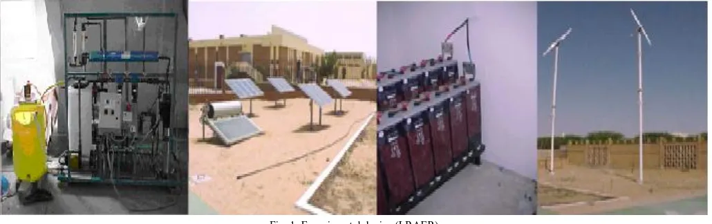
The experimental device existing at laboratory (LRAER) of Faculty of Sciences And Technology USTM of Nouakchott is an autonomous system, composed of a hybrid system of electrical production (wind turbine-photovoltaic-diesel) with 5.7 KW connected to a water desalination unit (osmosis reverses) along with other loads and secondary equipments (Figure 1)[4,5] .
Producing electric chain hybrid system consists of following elements:
Two aerogenerators: 1.5 kW and 3 kW Bornay mark, related to the continuous bus via a diode Inverted.
16 photovoltaic panels (1.2 kW) connected to the continuous bus.
A generator of 5 kW nominal power.
The energy storage device implanted in this hybrid system is connected directly to the continuous bus.
International Journal of Mechanical & Mechatronics Engineering IJMME-IJENS Vol:16 No:02 2
Fig. 1. Experimental device (LRAER)
3. GEOMETRICAL CHARACTERISTICS OF BORNAY3000 The knowledge of the geometrical characteristics of Bornay and the blades profile (Figure 2), allow for optimal energy conversion. It also allows for a better return on the aerodynamic forces. We are particularly interested in the
compartments in this blade, which is a twin-bladed propeller (n = 2) - subjected to different simulated wind speed at our site.
Fig. 2.Airfoil of the wind turbine blade (Bornay 3000) on Matlab
The table below gives the characteristics of the airfoil for four types of Bornay wind turbines, including Bornay3000[6]. However, we acknowledge the representation of the aerodynamic profile of the wind turbine Bornay3000 blade by Matlab. The simulation is based on the data of the machine profile.
Module A
(mm) B (mm)
C (mm)
D (mm)
E (mm)
Bornay600 1000 1120 350 360 1470
Bornay1500 1430 1670 370 470 2040
Bornay3000 2000 2140 470 645 2610
Bornay6000 2000 2640 495 645 3135
It is important to note that our blade profile is provided by Matlab. It is done with two parameters (X, Y), which summarize the characteristics of the aerodynamic profile of
the blades of the wind turbine (Bornay3000). This method of approximation of the profile is achieved with Bornay3000, which can serve for testing of optimization of the characteristics of this type of machine through different profiles of the blades in search of an optimization by Matlab tool.
4. MODELING
Regarding this part related to modeling of flows of fluids and in accordance with what is stated above, the general theory of the wind engine (turbine) with a horizontal axis has been established by Betz under the hypotheses following:
- Axial flow (air movement is not rotating)
- Incompressible flow,
- Air passing through the rotor without friction,
1 4 2 3
This theory is based on the following principles:
- The principle of conservation of mass
1 1 2 2 3 3 4 4
S V S V S V S V (2)
- Bernoulli's equation
2
1
2V Pgz cste
(3)
Applying Bernoulli's equation on the stations 1 and 2 (Figure 3) gives:
:
2 2
2 3 1 4
1 2
P P V V (4)
2 2
1 4
1 2
x
F PS S V V
(5)
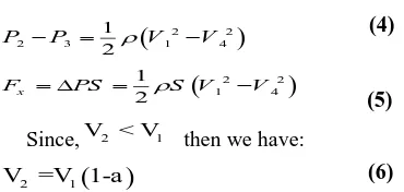
Since,V < V 2 1 then we have:
2 1
V =V 1-a (6)
Principle of change of momentum (from V of the air wind between upstream and downstream of the propeller) allows us to write the relations of force and mechanical power exerted on the blade:
1 4
ext
F mV m V V
(7)
x 2 1 4
F
V S V V (8)The equality of the two equations (5) and (8) gives the following expression:
1 4
2 4 1
V = V =V 1-2a
2 V V
et
(9)
Introducing the equation (9) in expression (8), we have the equation as follows in axial force:
2 21
2 1
x
F a a
V
r (10)Mechanical power is expressed as the equation:
2
2 2 1 4
r
P FV SV V V (11)
Next, we introduce the equations (9) and (10) into equation (11), to find equation (12):
2 2 3 1 1 4 1 2 extrP
r V a a (12)The power available from the wind depends on the area swept by the propeller of the wind wheel, the density of air and the wind velocity. We can express it as:
2 3 1 1
2
disp
P
r V (13)We obtain Cp depending on interference factor, hence, the following equation, which characterizes the efficiency and performance of the wind turbine, in the equation:
24 1 extr
p
disp P
C a a
P
(14)
The maximum value of the power coefficient (Betz limit) can be obtained by differentiating equation (14) and equating to zero, to obtain the equation (15):
1 0 3 p dC a
da
(15)
Under these conditions the power is maximum; it is given in the form of (16):
3
max 1
16 1 27 2
P SV (16)
Thus we get the Betz limit (Cp) in the equation (17) as:
216
100 4 1 59.26%
27 p
C a a
(17)
According to the theory of Betz, an aerodynamic performance of a wind turbine may not be higher than 59.26% (Betz limit). In practice, it has a yield of 50% in relation to the last wind turbines manufactured in Europe along with the minimum flow of interference through the blades.
5. SIMULATIONS
International Journal of Mechanical & Mechatronics Engineering IJMME-IJENS Vol:16 No:02 4
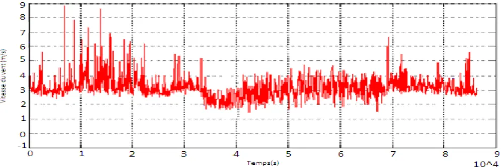
Fig. 4. Real speed of the wind on the site (LRAER)
Before starting the simulations, it is important to include in this part, the two parameters used in the mathematical model of the axial force (équation.10), these include the radius (R) and distribution of wind speed (V). These two parameters will be subjected to variations as a function of a (interfering factor). So it is important to know why the choice of their execution intervals for simulation.
For the first parameter, the manufacturer Bornay gives a wind speed in the interval of 2 to 20 m / s (Figure 5), wherein the average speed of the site is close to 4.3 m / s. The
manufacturer provides for a wind turbine power curves (see Figure 5), the minimum starting speed is 2 m / s and maximum speed as 25 m / s. These values correspond to modern wind turbines of small powers in the lower power range of 10 kilowatts (will not exceed 100). The gusts (Figure 4) given by the wind speed on the site (speed peaks for a very limited period of time) can reach 9 m / s. Then we will run the simulation, taking into account variations in the wind speed of the wind generator curve in the range of speeds recorded in LRAER [1-9 m / s] and an average fixed speed around 4.3 m / sec, given by the same data acquisition system.
Fig. 5. Curve of power for bornay3000
For the second parameter the radius of the blades is a substantial part of the wind wheel device. The yield of the proper function and machine life depends on its design. The radius of the blades given by the manufacturers of wind motors ranges from 1 m for the small wind turbine to over 2 m from the largest. Wind turbine generator rays can (in case the average power range) run around 275 Kw, reaching over 16m [example in Nouadhibou, Mauritania, we have Vergnet brand wind turbines (75 and 275 Kw)].
It should be noted that for a given wind speed, the power of the turbine proportional to the cube of the speed, as well as the power extracted by the wind turbine through the area swept by the blade, is _ proportional to the square of length of the
blade. The two parameters (V and R) interest us based on the modeled aerodynamic force in the axial interference factor (a). We are particularly interested in the influence of the two parameters through mathematical models.
5.1 Simulation Aerodynamic Force Based on the Interference Factor.
0 0.05 0.1 0.15 0.2 0.25 0.3 0.35 0
50 100 150 200 250 300 350 400
Facteur d'interference (a)
Fo
rce
a
xia
l (
N)
Fig. 6. Axial force in terms of a fixed radius (R = 2m) and velocity distribution V = [1: 9 m / s]
Figure 6 shows that the maximum is obtained by an interference factor of 0.333. The evolution curves quasi are identical in shape but have various values in amplitudes. They respond to the same points on the interference factor.
Physically this phenomenon can be translated as follows: for a given site and for our type of wind turbine; the maximum value of the axial force can be searched around the point of the interference factor of a value close to 0.333. So the wind speed plays a crucial role in the evolution of the axial force.
Axial force as a function of R = [1: 16 m] with (Vm = 4.3 m / s (constant)
The axial force is responsive to changes in the curves as a function of the interference factor, following any increase in the radius of the blades. It follows an increasing exponential shape with a maximum limit of around 6500N with a value of (a), close to 0.333. Then for each increasing radius value, we have a maximum corresponding to a maximum value of force at that point (a), close to 0.333. The axial force varies from O up to about 6500 N.
0 0.05 0.1 0.15 0.2 0.25 0.3 0.35
0 1000 2000 3000 4000 5000 6000 7000
Facteur d'interference (a)
Fo
rce
a
xi
al
(
N
)
Fig. 7. axial force with a function of a fixed wind speed (Vm = 4.3 m / s) and a blade radius distribution of R = [1: 16 m]
The maximums are registered with an interference factor of 0.333. The evolution curves are Quasi identical in shape but of different values and amplitudes. They respond to the same interference factor points, which are recorded for maximum axial force.
Physically this phenomenon can be translated as follows: for a
given site and for a type of wind turbine, the maximum value of the axial force can be found at the point of the interference factor (0.333). The blades of the radius play a key role in the evolution of the axial force.
International Journal of Mechanical & Mechatronics Engineering IJMME-IJENS Vol:16 No:02 6
0 0.05 0.1 0.15 0.2 0.25 0.3 0.35
0 20 40 60 80 100 120
Facteur d'interference (a)
Fo
rce
a
xi
al
(
N
)
Fig. 8. axial force with a function of a radius (R = 2 m) and speed V = 4.3m / s
Analysis of Figure 8 corresponds to the simulation of the equation (10). This shows that the aerodynamic force versus interference factor reaches a maximum value of 100N (a = 0.333). It maintains the same growth pattern as previous curves.
5.2 Simulating the Power of Wind Generators Based on the Interference Factor
For this part, the simulations are performed in the form of powers:
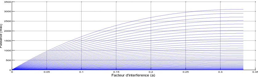
• Power of the wind turbine as a function of (a) with a fixed radius and variable speed ranging from[1-9 m / s] (Figure 9), • Power of the wind turbine as a function of (a) with a fixed wind speed (Vm = 4.3 m / s), by varying the radius of the blade (R) from 1 to 16 m (Figure 10),
• The power of the wind turbine as a function of (a) with a fixed radius (R = 2m) and a fixed average speed (V = 4.3 m / s) (Figure 11).
In this context, the analysis of these figures in accordance with equation (12), it is possible to say that the power of the wind turbine reacts to the same parameters (R and G) and follows the same physical laws. Figures 9, 10 and 11 are already recorded in Part 5.1 (Figures 6, 7 and 8). This means that by acting on these two parameters (R and V), we can increase or decrease the power of the wind turbine.
The power curve gives many variations:
• Figure 9: we record power variation for a fixed radius and variable speed in a range [1-9 m / s] with a maximum value (P maximum KW = 3) for a = 0.333;
• Figure 10: The simulation gives a very significant power versus interference factor.
• Figure 11: The analysis of this figure shows that the power versus interference factor reaches a maximum value of 320 Watt for a value (a = 0.333). It maintains the same growth pattern as previous curves.
0 0.05 0.1 0.15 0.2 0.25 0.3 0.35
0 500 1000 1500 2000 2500 3000 3500
Facteur d'interference (a)
P
ui
ssa
nce
(
W
at
t)
0 0.05 0.1 0.15 0.2 0.25 0.3 0.35 0
Facteur d'interference (a)
Fig. 10. Power of a wind turbine with a function of a fixed wind speed (average speed = 4.3m / s) and blade radius distribution of the R = [1: 16]
0 0.05 0.1 0.15 0.2 0.25 0.3 0.35
0 50 100 150 200 250 300 350
Facteur d'interference (a)
P
u
issa
n
ce
(
W
a
tt
)
Fig. 11. Power of a wind turbine with a function of a fixed radius (R = 2m) and fixed speed (average speed = 4.3m / s)
From this we found that the simulations follow a similar shape to an increasing exponential function. For figures (9, 10 and 11) respectively, we have shown that the maximum is obtained for an interference factor value of 0.333. The evolution curves Quasi are identical in shape but changes occur in amplitudes. They respond to the same points of interference factor.
Physically this phenomenon can be translated as follows: for a given site and for our type of wind turbine, the maximum value of the power can be found with the interference factor (0.333). The wind speed and radius play a key role in the evolution of the power of the machine.
International Journal of Mechanical & Mechatronics Engineering IJMME-IJENS Vol: 16 No: 02 8
5.3 Simulation of Profitability Based on the Interference Factor
0 0.05 0.1 0.15 0.2 0.25 0.3 0.35
0 10 20 30 40 50 60
Facteur d'interférence (a)
C
o
é
ff
ici
e
n
t
d
e
p
u
issa
n
ce
(
%
)
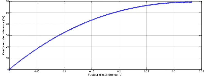
Fig. 12. Aerodynamic efficiency depending interference factor
The yield or performance of the wind turbine depends on its characteristic and the characteristic of the implantation site. For this, equation (17) was simulated. From the analysis of Figure 12 and equation (17), we conclude that the aerodynamic efficiency of the wind generator reaches a maximum value of 0.59 when the interference factor is a=0.333.
This result is in agreement with the Betz theory that says aerodynamic performance of a wind turbine may not exceed 59.26% (Betz limit).
6. DISCUSSIONS
The axial force or power, depending on (a) varies V or R, fixing the other parameters, evolves with the same laws that govern similar physical phenomena. We noted that the maximum axial force or power is registered for an interference factor close to (a = 0.333). The evolution curves are quasi identical in form, but at different values of evolution, especially those related to the amplitude.
Analyses of these figures are in conformity with the equations (10, 12) and that allow the power of the wind turbine and the axial force to react to the same parameters (R and G) and follow the same physical laws.
This means that by acting on these two parameters (R and V), we can increase or decrease the axial force and then act on the power of the wind turbine.
Thus, we have shown:
• The variation of the radius of the wind turbine blade has a direct influence on the force applied to the rotor and the power of the wind turbine,
• Increasing the speed of the wind acts directly on the axial force and the power of the wind turbine as a function of (a) when the radius is fixed,
• The power of the wind motor and profitability depend on the parameters (V and R) developed in this work.
These results show that the choice of the blades (length, aerodynamic shape), the site (wind speed) are important for the choice of the wind and its implementation option for the production of electricity. These two parameters (R and V) directly influence the axial force and therefore the power of the wind turbine and profitability.
In effect, the power produced by the wind turbine changes proportionally according to the variation of the radius squared of the blades and the wind speed cubed (equation 12). This displays the power and a similarity of action with the axial force. The axial force follows the same physical laws that the evolution of the power produced by the wind turbine; based on the interference factor and parameters (R and G) on production. The axial force varies remarkably with these two parameters as well as the power and efficiency of the turbine.
7. CONCLUSION
We presented a paper on the general theory of the wind engine (turbine) with horizontal axis that was established by Betz [5 and 6] under the following assumptions: axial flow (air movement is not rotating), flow is incompressible and air is passing through the rotor without friction.
Similarly, we have created a representation of the aerodynamic profile of the blade of Matlab wind turbine Bornay3000 (Figure 2). We also developed mathematical models through the physical laws of fluid flow on an aerodynamic shape to find Cp power coefficient and thereafter introduced the modeling portion with both parameters involved, the first time being in the axial force and the second time in power. These include the radius (R) and the wind speed (V). Precisely, the power and the axial force are subject to variations as a function of a, in the simulation.
the behavior of this interaction and give suggestions about the sifting of wind turbines in any site and understand the influence of the interference factor on the profitability and productivity of the wind turbine.
ACKNOWLEDGMENTS
Thanks to Larbi El Bakkali and Abdel Kader Mahmoud, who are responsible for the Modeling and Simulation Laboratory of Mechanical Systems, FS-Tetouan, UAE and the chef of the Laboratory for Applied Research in Renewable Energy, FST, USTM. A big thanks to all the members of these two laboratories for their active collaboration in scientific research.
REFERENCES
[1] S. Liu et I. Janajreh, « Development and application of an improved blade element momentum method model on horizontal axis wind turbines », Int. J. Energy Environ. Eng., vol. 3, no 1, p.
30, oct. 2012.
[2] D. Wood, « Blade Element Theory for Wind Turbines », in Small Wind Turbines, Springer London, 2011, p. 41‑55.
[3] A. F. Akon, « Measurement of Axial Induction Factor for a Model Wind Turbine », août 2012.
[4] B. Ould Bilal, V. Sambou, P. A. Ndiaye, C. M. F. Kébé, et M. Ndongo, « Optimal design of a hybrid solar–wind-battery system using the minimization of the annualized cost system and the minimization of the loss of power supply probability (LPSP) », Renew. Energy, vol. 35, no 10, p. 2388‑2390, oct. 2010.
[5] Ahmed Mohamed Yahya, Adel Mellit, Abdel Kader Mahmoud, Issaha Youm, « Lead-Acid Battery Behavior Modelling and Experimental Validation Under a Specific Climatic Condition for a Hybrid Solar-Wind System », International Review on Modelling and Simulations (IREMOS), vol. 4, no 4, p.1751-1759, August 2011.
![Fig. 7. axial force with a function of a fixed wind speed (Vm = 4.3 m / s) and a blade radius distribution of R = [1: 16 m]](https://thumb-us.123doks.com/thumbv2/123dok_us/1357635.1644731/5.612.99.517.489.627/axial-force-function-fixed-speed-blade-radius-distribution.webp)
![Fig. 10. Power of a wind turbine with a function of a fixed wind speed (average speed = 4.3m / s) and blade radius distribution of the R = [1: 16]](https://thumb-us.123doks.com/thumbv2/123dok_us/1357635.1644731/7.612.100.519.259.418/power-turbine-function-fixed-average-blade-radius-distribution.webp)