ORIGINAL PAPER
An activity-based approach for complex travel
behaviour modelling
Gennaro Nicola Bifulco&Armando Cartenì& Andrea Papola
Received: 4 June 2009 / Accepted: 2 November 2010 / Published online: 16 November 2010 #The Author(s) 2010. This article is published with open access at Springerlink.com
Abstract
Purpose In this paper an activity-based modelling
frame-work is presented. It enhances many of the characteristics of existing approaches and enables a more accurate travel demand modelling.
Methods The model approach proposed explicitly takes
into account the households’role, as well as time and space constraints. Issues related to activity participation and activity planning are explicitly addressed with respect to the horizon of a whole week. The proposed framework allows to reproduce activity lists and activity patterns in an explicit and consistent way. As a consequence, time and mode characteristics of travel demand are more accurately computed. The approach has been designed in order to capture interactions among households members and to explicitly represent trip-chains and relationships between trips within activity patterns. In this paper a comprehensive formalisation of the modelling framework is presented and part of it is estimated on the basis of ad-hoc collected data.
Application The modelling framework has been then
applied to the Naples’metropolitan area (southern Italy), a catchment area with about three million inhabitants.
Results and Conclusions The proposed framework has
shown a satisfying flexibility, as well as a good ability in reproducing real data. It seems to be a good compromise between accuracy and operative issues, which improves the range of reproducible mobility phenomena and the accuracy of this reproduction and at the same time it moves some step forward the practical applicability of activity-based approaches.
Keywords Activity-based . Demand model . Travel behaviours . Nested logit . Transport model . RP survey
1 Introduction
As known, travel demand derives from the need to carry out activities in multiple locations. In the last decades, the increased economic and social welfare has drastically changed the shape of our style-of-life and induced an increasing complexity in our activity patterns and travel behaviours. As a consequence an increased congestion can be observed also in off-peak periods and often across the whole day. The main implication of this increased com-plexity is the need of modelling the whole day and using, at this aim, more complex and rigorous travel demand modelling approaches.
Thetrip-basedapproach is certainly the most simple and popular. It approximates mobility phenomena by consider-ing one-way trips. In other terms, all trips carried out by individuals in the whole day are modelled independently from their reciprocal relationships. An early example of a comprehensive trip-based approach was developed by the MTC (Metropolitan Transportation Commission) for the San Francisco Bay Area [1]. Other relevant examples can be found in [2] and in [3]. In [4] Horowitz presented a trip G. N. Bifulco
Via Claudio 21, University of Naples, Naples 80100, Italy
e-mail: [email protected]
A. Cartenì (*)
Via Ponte Don Melillo, University of Salerno, Fisciano, SA 84084, Italy
e-mail: [email protected]
A. Papola
Via Claudio 21, University of Naples, Naples 80100, Italy
frequency, destination and mode choice modelling work able to incorporate (still within a trip-based frame-work) some inter-trip dependencies.
Thetrip chainingapproach is able to represent relation-ships between the different trips that constitute an individ-ual travel chain, and thus considerably generalize conventional trip-based models. Trip-chain models have been studied for several years; however, they have been rarely implemented in real contexts and seldom in complex urban areas. Early examples can be found in late 1970s (see for instance [5]). Relevant experiments have been made in 1980s in Netherlands [6, 7]. Relatively more recent trip-chain modelling frameworks have been developed for Stockholm [8] and Salerno [9]. However, the trip-chain approach does not address the fundamental factors that determine the actual configuration of particular trip chains and round trips. To address such questions, it is necessary to explicitly consider the activities that individuals and households undertake, and that give rise to transportation demand.
The activity-basedapproach just derives travel patterns from a representation of these more basic activities by taking into account the interaction among individuals participating to the same set of activities as well as all temporal and physical constraints among single trips. Jones in [10] has defined some characteristics that an activity-based model should have:
1. travel demand should be treated as a derived demand; 2. activity sequences should be considered, rather than
trips or trip-chains;
3. households should be considered as decision-making units;
4. spatial and temporal constraints should be explicitly taken into account;
5. activity scheduling over time and space should be considered.
In past years significant efforts have been devoted to refine the activity-based theory. However, few consistent specifications have been presented and most of them are not suitable from an operational standpoint and/or are incom-plete with respect to the representation of all the Jones’ implications. In [11] some aspects related to activity duration (time-budgeting) and activity scheduling have been addressed through coupled discrete/continuous choice models. In [12] day-to-day variations in travel patterns have been analysed and in [13] activities and travel choices within a weekly activity pattern have been modelled. In [14] an activity-based-like approach has been restricted to trip generation, while in [15] the aim of the analysis has been restricted to deal with consistency issues in mode-choices within sequences of trips. In [16] enhanced methods for modelling activity duration have been
intro-duced while in [17] a model specification has been proposed addressing most of the Jones’ topics. Other relevant contributions to the development of the activity-based approach can be found in [18–24].
The attempt of this paper is to move a further step toward an advanced and comprehensive formulation of the activity-based approach, allowing for a better simulation tool for the estimation of demand matrices. The paper is organized in four sections. Section 2 shows an example clarifying the main limits ofnon activity-basedapproaches. In Section 3 a comprehensive theoretical activity based framework trying to overcome all these limits is proposed. In Section 4 part of the proposed modelling framework is estimated on the basis of ad hoc collected data and then applied to a real case study. Section 5 reports some conclusive remarks.
2 Limits of non activity-based approaches
This section shows an example aimed at clarifying the main limits and errors of non activity-based approaches in reproducing complex transport behaviours.
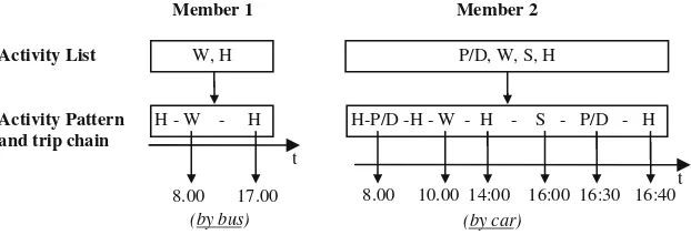
Consider a household composed by a couple of young employees with two children. Assume they own one car and have to carry out the following activities in a given work-day: – working (W); both household members work; one for 8 h a day (8:00 to 16:00) and the other for 4 h a day (10:00 to 14:00);
– shopping at supermarket (S);
– pick up and delivering of children at (the same) school (P/D);
The activity list is completed by adding the staying at home activity (H). Assume the planning of daily activities for member 1 of the household (8 h working-time) consists in driving children school, going work and after work taking children back, going to the supermarket and finally coming back home. In the meanwhile, members 2 (4 h working-time) goes working by bus and after work comes back home. The resulting activity lists, activity patterns and the related trip-chains are summarised in Fig. 1.
For sake of simplicity, trip durations are not explicitly depicted in the previous figure; these are assumed to be somehow included within the activity durations. Transport modes for any trip-chain are indicated in the figure.
This example is useful in order to show how a congestion increase in a time slice of the day could cause change in the daily individual activity lists of a household and, consequently, in the activity patterns and trip chains of each individual. The result can be a significantly different number of trips (a counterintuitive increase, in this example), carried out in different periods of the day and with different modes (in the example with a counterintuitive increased use of the car).
It is worth noting that such a complex behaviour can be managed only through a fully deployed activity-pattern approach which endogenously deals with activity lists and activity patterns.
A (even sophisticated) trip-chain approach could repro-duce, at most, how the above-mentioned increase of congestion can influence the trip chain organization of each individual (trip chains vs. round trips), as wtime-period and mode choices of secondary activities (P/D, S). It is worth noting that the final result could have been in our example a tout-court reduction of car use due to the increase of congestion, which is not the same result obtained by using the activity-based approach. Moreover, the reallocation of activities as well as of the car availability from one member of the household to the other cannot be reproduced by a trip-chain approach, with a consequent unsatisfactory modelling of the actual mobility of the whole household.
A trip based approach is even more limited since it could reproduce, at most, frequency and car use reduction for trips in the congestion period (for P/D and S activities), without considering at all how this congestion could influence the mobility pattern in different time-periods of the day.
In the next section an activity-based approach is formalised with the aim of addressing all issues highlighted by the previous example.
3 A theoretical reference framework
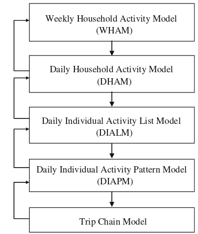
In this section a possible theoretical formulation for the specification of a system of models in activity-based-style will be presented. The overall structure of the proposed framework is shared by several models and is shown in Fig.3.
This particular architecture aims to explicitly model all travel phenomena related to activity pattern and travel choices: from household weekly activities to individual single trips. It is composed by five sub-models:
1. Weekly Household Activity Model (WHAM), which
reproduces the number and types of activities carried out by households within a week;
2. Daily Household Activity Model (DHAM), which
reproduces the distribution of all household activities over days of the week;
3. Daily Individual Activity List Model (DIALM), which
distributes daily activities among the household com-ponents;
4. Daily Individual Activity Pattern Model (DIAPM),
which combines the individual daily activities leading to actual activity patterns and related trip-chain sequences;
5. Trip chain Model, which reproduces the organization of
all trips provided within an activity pattern.
Figure3shows that each level is related to the previous and subsequent. The three upper levels refer to longer term
Activity List
Activity Pattern and Trip Chain
Member 1 Member 2
P/D, W, S, H W, H
(by car) (by bus)
H - P/D - W - P/D - S - H
7:30 8:00 16:30 16:40 17:00t
H - W - H
10.00 14.00 t Fig. 1 Activity lists, activity
patterns and trip-chains of the reference day
Activity List
Activity Pattern and trip chain
Member 1 Member 2
W, H P/D, W, S, H
H - W - H H-P/D -H - W - H - S - P/D - H
8.00 17.00 8.00 10.00 14:00 16:00 16:30 16:40
(by bus) (by car)
t
t Fig. 2 Activity lists, activity
decisions, they reproduce the activity organization among household members in a fixed period of time. The latter two levels represent shorter term travel decisions. All the models of the overall framework will be formalised in this section, while in Section4 the DIAPM and the Trip-chain models will be specified and estimated through ad-hoc collected data.
3.1 Weekly household activity model
The model aims to reproduce the whole set of activities carried out by a household within a week.Given a list of possible activities (work, study, shopping, sport, etc.), the generic alternativewiis given by the set of activities carried out by a household of typei within a week. Formally we may write:
wi¼ ðxiw;1;xiw;2;. . .;xiw;a;. . .;xiw;naÞ
8i2 f1;2;. . .;nhg 8wi2 f1;2;. . .;Cig
ð1Þ
where:
xi
w;a is the number of times that an activity of type ais
performed by householdiwithin a week in alternativew
na is the number of possible activities
nh is the number of different household types
Ci is the choice set i.e. the set of all possible weekly sets of activities for householdi.
Just as an example, alternativewicould be composed by: xi
w;1¼12 work activities, xiw;2¼8 study activities and so
on (assuming, for instance, that 1 stands forWorkand 2 for Study).
Relevant attributes are the household’s characteristics and may include the number and age of employed adults, the number and age of non-adults, the dwelling-place, income, number of driving licences, number of cars, etc. as well as a logsum variable related to the lower choice dimensions.
3.2 Daily household activity model
In this case the model aims to reproduce how the set of weekly activities identified by the previous model is split into daily activity sets. The generic alternative di
g=w, is
given by any set of daily activities consistent with the weekly set of activities wi. Formally we may write:
di
g=w¼ ðxig=w;1;xig=w;2;. . .;xig=w;a;. . .;xig=w;naÞ
8g2 1;2;. . .;ng ¼7
ð2Þ
where:
ng(=7) is the number of days in a week
xig
=w;a is the number of times that an activity of type a is carried out during dayg by the household of typeigiven the weekly household set of activitiesw;
and the following constraints have to be satisfied:
Png
g¼1 xi
g=w;a¼xiw;a 8a2f1;2;. . .;nag;
8wi2Ci;8i2 1;2;. . .;n h
f g ð
3Þ
For example if, as in the previous example,xiw;1¼12 work activities,xi
w;2 ¼8 study activities, the following conditions
have to be satisfied:
P7
g¼1 xi
g=w;1¼12;
P7
g¼1 xi
g=w;2¼8 1¼Work;2¼School
Constraints (3) implicitly define the choice set Ci
g=w of this
choice dimension. However, it is useful in practical imple-mentation to reduce the combinatorial complexity of the problem by dropping out unlike alternatives Relevant attrib-utes are in principle similar to those of the previous models.
Note that the model can be also formalized in an aggregate way by defining the average weekday (holiday) gwdðghdÞ. In this case the generic alternative becomes: dig=w¼ ðxig=w;1;xig=w;2;. . .;xig=w;a;. . .;xgi=w;naÞ ð2bÞ and constraints (3) become:
5xi
gwd=w;aþ2xighd=w;a¼xiw;a 8a2f1;2;. . .;nag;
8wi2Ci;8i2f1;2;. . .;nhg
ð3bÞ Weekly Household Activity Model
(WHAM)
Daily Household Activity Model (DHAM)
Daily Individual Activity List Model (DIALM)
Daily Individual Activity Pattern Model (DIAPM)
Trip Chain Model
where5and2are the number of weekday and holiday in a week respectively.
3.3 Daily individual activity list model
This sub-model reproduces the distribution of daily activities among the components of a household. This leads to daily individual activity lists which are the starting points for reproducing the daily travel choices of each individual. In this case the generic alternativeki
r=g;wis given
by the daily activity list of each componentrof household i, i.e. types and numbers of activities he/she carries out during a dayggiven the daily set of household activities dg/w:
kri=g;d
g=w ¼ ðx
i
r=g;dg=w;1;. . .;x
i
r=g;dg=w;a;. . .;x i
r=g;dg=w;naÞ
8r2 f1;2 . . .;nirg
ð4Þ
where:
xi
r=g;dg=w;a is the number of times that an activity of typeais carried out by componentrof householdiin day g, given the daily set of household activitiesdg/w
ni
r is the number of components of the typei
household
and the following constraints have to be satisfied:
Xni r
r¼1
xir=g;dg=w;a ¼xig=w;a8a2f1;2;. . .;nag;
8g 2 1;2;. . .;ng¼7
;
8wi2Ci;8i2f1;2;. . .;nhg
ð5Þ
Once again, constraints (5) implicitly define the choice set of this sub-model Ci
r=g;w
but in order to reduce the combinatorial complexity of the problem, this can be reduced by dropping out unlikely activity lists.
Relevant attributes are also in this case similar to those of the previous models but concern the specific individual and obviously include gender and occupation-al status.
Also in this case the model can be formalized in an aggregate way by considering the average day g. In this case the generic alternative becomes:
kir=g;d
g=w ¼ ðx
i
r=g;dg=w;1;. . .;x
i
r=g;dg=w;a;. . .;x i
r=g;dg=w;naÞ
8r2 f1;2 . . .;ni rg
ð4bÞ
and constraints (5) become:
Xni r
r¼1 xir=g;d
g=w;a ¼x
i
g=w;a 8a2f1;2;. . .;nag;8wi2Ci;
8i2f1;2;. . .;nhg
ð5bÞ
3.4 Activity pattern and trip chain models
This model reproduces how different activity patterns can be generated from a given daily individual activity list. Figure4exemplifies some possible activity patterns (right) which can be generated from a given daily individual activity list (left). The generic alternative pir=k;g;d
g=wrepresents the generic activity pattern π of component r of household i given the daily individual activity list k of the dayg, the daily set of household activities d and the weeky set of household activities w.
It is worth noting that the daily individual activity list provides the number of times each activity is carried out within the day (one in Fig.4), except forhomewhich can be repeated several times. The number of times (minus one) activity homeis repeated in a given activity pattern implicitly determines the number of trip-chains related to that activity pattern. For instance, three chains are associated to the second activity pattern in Fig. 4 (H-P/ D-O-H-W-H-L-H) since activity home is replicated four times.
Also in this case the number of possible activity patterns which can be associated to each activity list can be reduced by considering only those which are chosen with a significant frequency in the sample.
Relevant attributes are also in this case socio-economic characteristics of the individual. The logsum variable related to the subsequent trip chain model includes the generalized costs of the different chains. Therefore the choice of the activity pattern is influenced by the network congestion at different times of the day.
Also in this case the model can be formalized in an aggregate way by considering the average day g. Given an activity pattern (i.e. a given succession of trip chains), the role of the trip chain model is to reproduce when and how these trip chains are carried out within the day, introducing not only consistency within the generic trip chain but also among the different chains of the day, mainly in terms of activity duration and departure time. More details about these internal and external consistencies will be given in the following sections.
4 Specification, calibration and application
Although all the proposed architecture could consistently use the discrete choice approach, the first three sub-models
(WHAM, DHAM and DIALM) have been estimated
exog-enously according to a descriptive approach, following the results of a survey conducted on the Naples metropolitan area; this means that the results of the first three models are given and fixed.
According to the survey results, the activity patterns that have been verified as feasible (i.e., that are actually observed in the sample) consist either in home-based trip-chains or double tours. The incidence of more complex patterns was found to be negligible for workers in the Naples area.
A disaggregate estimation of activity pattern (DIAPM) and time-of-day choice models was performed, while an aggregate estimation (parameter updating) of destination and mode choice models was carried out starting from the results of a disaggregate calibration available for Naples demand models ([25]). The validation tests used are theρ2 and the t-student for the disaggregate calibration and the
Mean Absolute Percentage Deviation (MAPD) for the
aggregate one.
4.1 The survey
A fundamental aspect for the specification, calibration (parameter estimation) and implementation of a system of activity-based models is a properly designed database which can describe the observed pattern of urban travel mobility. The model system was specified and calibrated
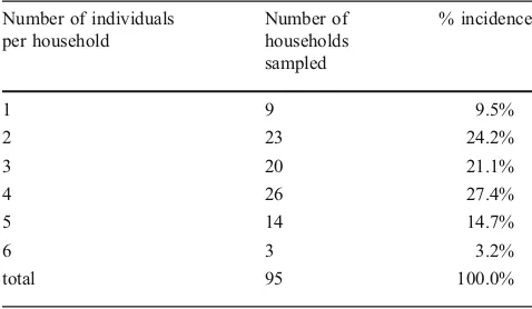
from a complex survey (extended overtime) carried out in the metropolitan area of Naples. A complex methodology was followed to collect extensive information, since travel and activity choices information must be gathered for all individuals of a household and for all the days of a week. The aim of the survey was to find out the household’s and individual’s “diary” throughout an entire week, in order both to analyse the phenomenon and generate a database for model specification and estimation. The sample consists of roughly 100 households, comprising 300 individuals, in the Naples urban area, who were asked about all their activities during a given week.
Some of the most significant results are reported briefly in the following tables. In particular, in Table 1, the percentages of households with different number of components are shown. As it can be seen, most of the households include 2, 3 or 4 components (24%, 21% and 27% of the households sampled respectively).
In Table 2, the average number of weekly activities per household typology are reported, distinguishing between in-house and out-door activities. As it can be seen, the total number of activities carried out on average by a single component of the household is quite independent by the number of components of the household: for example it is 29 for single households and about 28 for two, three and four-components households.
In Table 2, the average number of weekly activities per household typology are reported, distinguishing between in-house and out-door activities. As it can be seen, the total number of activities carried out on average by a single component of the household is quite independent by the number of components of the household: for example it is 29 for single households and about 28 for two, three and four-components households.
Concerning the in-house activities it can be observed
that personal care and Housework activities are more
frequently carried out by single component households (4 weekly activities which represent the 36% of the total weekly activities). By contrast, 6 components households carry out these kind of activities 14 times in a week on average (i.e. 2.3 per person) which represent the 21% of the total weekly activities. An opposite trend can be observed for leisure activities which represent the 9% of ACTIVITY LIST
1 W (WORK) 1
1 1
- H (HOME)
ACTIVITY PATTERNS H – A – W – H – L – O – H
H – A – O – H – W – H – L – H
H – W – A – O – L – H
H – L – W - H – O – H – A – H
H – W – H – L – O – H – A – H L (LEISURE)
A (ACCOMPANYING) O (OTHER)
Fig. 4 Activity pattern produc-tion from a given activity list
Table 1 Sample characteristics
Number of individuals per household
Number of households sampled
% incidence
1 9 9.5%
2 23 24.2%
3 20 21.1%
4 26 27.4%
5 14 14.7%
6 3 3.2%
the total weekly activities for single component house-hold, the 16% for 2 components households, the 25% for 3, 4, and 5 components households and the 45% for 6 components households.
Concerning the out-door activities it can be observed that single component households carry out, on average, a higher percentage of work activities (33% versus about 20% for the other typology of households). Also in this case, leisure activities are carried out more frequently by households with higher number of components (11% and 13% for one and two components households respectively and about 20% for the others households typology).
Finally, Table 3 shows the activity patterns which are more frequently chosen by the workers in the sample.
As shown in the table, the most selected activity pattern in the sample is a H-W-H simple tour with work purpose (28.5%). Also the double tour with work purpose H-W-H-W-H has a high percentage, (14.9%). These results show that most of the workers perform only work-based trips. Moreover, the first five activity patterns represent more than the half of the sample and each of the other activity patterns (not reported in the table) are chosen by less than the 2% of the sample.
Table 2 Average number of weekly activities per household and number of components
Number of individuals per household Total
1 2 3 4 5 6
In-house activities
Work 0 (0%) 1 (4%) 1 (2%) 2 (4%) 1 (2%) 0 (0%) 5 (2%)
Study 0 (0%) 4 (16%) 6 (14%) 9 (16%) 11 (21%) 8 (12%) 38 (15%)
Personal care and housework
4 (36%) 6 (24%) 12 (29%) 17 (31%) 15 (29%) 14 (21%) 68 (27%)
Leisure 1 (9%) 4 (16%) 11 (26%) 14 (25%) 13 (25%) 30 (45%) 73 (29%) Meal preparation 3 (27%) 4 (16%) 5 (12%) 6 (11%) 6 (12%) 4 (6%) 28 (11%)
Other 3 (27%) 6 (24%) 7 (17%) 7 (13%) 6 (12%) 11 (16%) 40 (16%)
Tot. in-house activities 11 (100%) 25 (100%) 42 (100%) 55 (100%) 52 (100%) 67 (100%) 252 (100%) Out-door
activities
Work 6 (33%) 6 (20%) 6 (14%) 11 (20%) 10 (18%) 18 (23%) 57 (21%)
Study 3 (17%) 6 (20%) 7 (17%) 11 (20%) 11 (20%) 18 (23%) 56 (20%)
Shopping 1 (6%) 2 (7%) 4 (10%) 4 (7%) 3 (5%) 2 (3%) 16 (6%)
Food purchase 1 (6%) 3 (10%) 5 (12%) 5 (9%) 5 (9%) 5 (6%) 24 (9%)
Sport 1 (6%) 1 (3%) 1 (2%) 2 (4%) 3 (5%) 3 (4%) 11 (4%)
Leisure 2 (11%) 4 (13%) 8 (19%) 10 (18%) 12 (22%) 14 (18%) 50 (18%) Pick up and Delivery 0 (0%) 3 (10%) 2 (5%) 3 (5%) 2 (4%) 7 (9%) 17 (6%)
Restaurant 2 (11%) 1 (3%) 2 (5%) 2 (4%) 1 (2%) 1 (1%) 9 (3%)
Other 2 (11%) 4 (13%) 7 (17%) 8 (14%) 8 (15%) 9 (12%) 38 (14%)
Tot. out-door activities 18 (100%) 30 (100%) 42 (100%) 56 (100%) 55 (100%) 77 (100%) 278 (100%)
total 29 55 84 111 107 144 530
Table 3 Worker activity patterns
Id. Activity-patterns % Activity
1 H-W-H 28.5% H Home
2 H-W-H-W-H 14.9% W Work
3 H-W-H-L-H 4.7% L Leisure
4 H-W-H-P/D-H 3.3% P/D Pick up and Delivery
5 H-W-H-O-H 2.7% O Other
Total 54.2%
activity pattern choice
first tour time-of-day choice
first tour destination choice
first tour mode choice
second tour time-of-day choice
second tour destination choice
second tour mode choice
DIAPM
Model
Trip Chain Model
4.2 Model specification and calibration
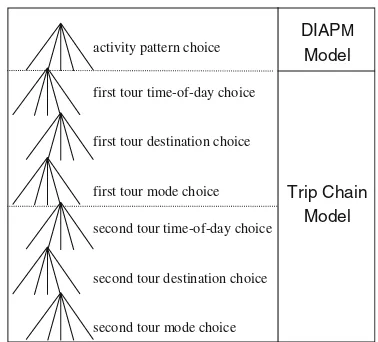
The choice dimensions considered for the application are (see Fig.5):
& activity pattern choice (DIAPM);
& tour choices (trip-chain Model), consisting in: (a) first tour:
(i) time-of-day choice; (ii) destination choice (iii) mode choice (b) second tour
(i) time-of-day choice; (ii) destination choice; (iii) mode choice.
As stated above, in order to simplify the application, the survey results have been used to reduce the model choice sets. In particular, the choice set of the activity pattern model is that reported in Table1.
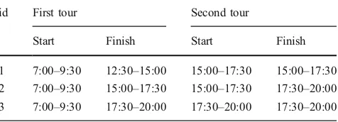
The alternatives considered for the time-of-day choice of the trip-chain model (first and second tour) are shown in Table4. Both for the first tour and for the second, a timeframe has been considered in which the individual could undertake his/ her tour and activity. As regards the morning departure time for the first tour, a single timeframe (7:00–9:30) has been considered, according to what observed in the sample.
For the destination choice models (both for the first and second tours) the Naples urban area has been divided into 16 macro-zones representing the major districts, while for the mode choice models three alternatives have been taken into account: car, public transport (bus, metro, funicular, rail and pedestrian) and motorbike. The whole modelling system exhibits a Nested-Logit structure. Accordingly with the formalization used in Section 3, the following sub-models are considered:
(DIAPM)
& activity pattern choice model, reproduces the choice of the activity patternπ(withπ∈{1,2,3,4,5} see Table3) for each origin zone o (with o∈{1,2,…,16}); for the level of aggregation considered in the application the notation introduced in Section3.4was simplified;
(Trip-Chain Model)
& first tour time-of-day choice model, reproduces the choice of the time-of-day I1for the first tour (with I1 ∈{1,2,3} see Table4);
& destination choice model for the first tour, reproduces the choice of the first destination d1 (with d1 ∈{1,2, …,16});
& mode choice model for the first tour, reproduces the choice of the modem1for the first tour (withm1∈{car,
public transport, motorbike});
& second tour time-of-day choice model, 8p6¼1 repro-duces the choice of the time-of-day I2 for the second tour. The choice set of this choice dimension is considered a function of the time constraints of the first tour (if the first tour has not ended, the second cannot start): I2≡3 ifI1=3;I2∈{1,2,3} otherwise (see Table4); & destination choice model for the second tour,8p6¼1
reproduces the choice of the second destination d2. Because the time-of-day 1 and 3 (Table 4) for the second tour have a limited time window (150 min), the choice set of this choice dimension d2was constrained
in the following way:
d2∈{1,2,…,16} ifI2=2 otherwise
d2∈{1,2,…,16}:Yo,d2,I2,π,I1,d1,m1≤0.097 otherwise;
where Yo,d2,I2,π,I1,d1,m1is the mode choice logsum variable of the second tour (see Tables 5and 6), related to theo-d2 pair, the time-of-day for the second tour I2, the activity pattern π, the time-of-day I1, the destination d1 and the mode m1. The value 0.097 was estimated jointly with the other model parameters. This estimated value corresponds to an average car/motorbike travel time of about 30 min and an average public transport travel time of about 40 min. In this way the destination choice set was considered a function of transport accessibility;
& mode choice model for the second tour, 8p6¼1 reproduces the choice of mode m2 (with m2 ∈{car, public transport, motorbike}) for the second tour.
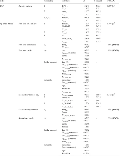
For the specification of the system of models we considered socio-economic, level-of-service and dummy variables. In Table 5 model attributes, model parameters and validation tests are reported. In Table 6 the attributes used are described.
With respect to the activity pattern choice model, the attributes used seek to highlight different observed behav-iour between males and females, since females are more likely to make second tour with other than work purpose or to come back home for lunch (H-W-H-L-H, H-W-H-P/D-H, H-W-H-O-H), while males either do the simple work-tour (H-W-H), which is the most widely chosen activity pattern, or the double work-tour (H-W-H-W-H).
Table 4 Time-of-day alternatives (first and second tour)
id First tour Second tour
Start Finish Start Finish
Table 5 DIAPandtrip-chainmodel: attributes, parameters and validation tests
Model Alternative Attribute βi t_student ρ2/MAPD
DIAP Activity patterns 1 H-W-H 3.241 4.135 0.289 (ρ2)
Yo,π 1.422 1.512
2 maleo 1.677 4.855
Yo,π 1.422 1.512
3, 4, 5 femaleo 0.675 1.906
Yo,π 1.422 1.512
Trip-chain Model First tour time-of-day 1 femaleo 1.374 3.744 0.197 (ρ2)
NoWork2 1.337 3.435
Yo,π,I1 1.452 2.713
2 Yo,π,I1 1.452 2.713
3 π1 1.303 3.852
work_owno 2.818 2.986
Yo,π,I1 1.452 2.713
First tour destination d1 Empd1 0.982 – 19% (MAPD)
Yo,d1,π,I1 0.587
First tour mode car car 0.713 – 12% (MAPD)
To,d1,I1(minutes) −0.032
centre −2.296
Yo,d1,m1,π,I1 0.221
Public transport fare (€) −0.002 –
Tbo,d1,I1(minutes) −0.037
Two,d1,I1(minutes) −0.021
Tpo,d1(minutes) −0.013
Ntrno,d1,I1 −0.307
Yo,d1,m1,π,I1 0.221
motorbike motorbike −1.381 –
Tmo,d1(minutes) −0.007
ageo 0.631
ExtraUrb −2.314
Yo,d1,m1,π,I1 0.221
Second tour time-of-day 1 Yo,I2,π,I1,d1,m1 0.077 0.667 0.342 (ρ2)
2 managero 1.031 2.155
Yo,I2,π,I1,d1,m1 0.077 0.667
3 π_NoWork 1.776 3.365
Yo,I2,π,I1,d1,m1 0.077 0.667
Second tour destination d2 Empd2 0.401 – 25% (MAPD)
Szone 0.651
Yo,d2,I2,π,I1,d1,m1 0.604
Second tour mode car car 0.713 – 22% (MAPD)
To,d2,I2(minutes) −0.032
centre −2.296
Smode 1.651
Public transport fare (€) −0.002 –
Tbo,d2,I2(minutes) −0.037
Two,d2,I2(minutes) −0.021
Tpo,d2(minutes) −0.013
Ntrno,d2,I2 −0.307
motorbike motorbike −1.381 –
Tmo,d2(minutes) −0.007
ageo 0.631
The attributes used for the first tour time-of-day choice model allow the observed data to be reproduced satisfyingly; part-time workers (especially female) choosing double tours, with non-work second tours (W-L-H, W-P/D-H, H-W-H-O-H), prefer the first timeframe (7:00–9:30/12:30–
15:00) for the first tour, while workers who choose the single tour (H-W-H) prefer or are forced to choose the last timeframe (7:00–9:30/17:30–20:00) for the second tour.
With respect to the second tour time-of-day choice model the calibration results, consistently with the observed
Table 6 DIAPandTrip-chainmodel: attribute description
H-W-His an alternative specific attribute related to the activity pattern 1: Home–Work–Home;
Yo,πis the logsum variable corresponding to the first tour time-of-day choice model, related to origin zoneoand activity patternπ
maleois a dummy variable of value 1 if the worker is male, 0 otherwise; this attribute reproduces the preference of male workers of choosing
activity pattern 2: Home–Work–Home–Work–Home
femaleois a dummy variable of value 1 if the worker is female, 0 otherwise; this attribute reproduces the preference of women of choosing activity
patterns with more than one activity and starting their activities early in the morning.
NoWork2is a dummy variable of value 1 if the activity patternπconsists of two tours without a work activity in the second tour (π∈{3,4,5}), 0
otherwise
Yo,π,I1is the logsum variable corresponding to the first tour destination choice model, related to origin zoneo, activity patternπand time-of-dayI1
π1is a dummy variable of value 1 if activity patternπ=1(Home–Work–Home), 0 otherwise; this attribute reproduces the preference of choosing time-of-day 3 (start: 7:00–9:30; finish: 17:30–20:00) forH-W-Hworkers
work_ownois the work on one’s own percentage in origin zoneo; this attribute reproduces the preference of this class of workers to work till late
in the afternoon (and thus finish the tour between 17:30 and 20:00)
Empd1is the logarithm of the number of employees at destinationd1; this attribute is representative of zoned1attractiveness
Yo,d1,π,I1is the logsum variable corresponding to the first tour mode choice model, related to origin zoneo, destinationd1, activity patternπand
time-of-dayI1
caris an alternative specific attribute
To,d1,I1is the car travel time (in minutes) from origin zoneoto the first destinationd1(and return) during time-of-dayI1
Centreis a dummy variable of value 1 if destinationd1is inside the city centre, 0 otherwise; this attribute reproduces the disutility of choosing the
car mode for reaching the city centre (caused for example by parking difficulties)
Yo,d1,m1π,I1is the logsum variable corresponding to the second tour time-of-day choice model, related to origin zoneo, destinationd1, modem1,
activity patternπand time-of-dayI1 fareis the public transport fare (in€)
Tbo,d1,I1is the public transport on-vehicle time (in minutes) from origin zoneoto the first destinationd1(and return) during time-of-dayI1
Two,d1,I1is the stops waiting time (in minutes) from origin zoneoto the first destinationd1(and return) during time-of-dayI1
Tpo,d1is the pedestrian walking time (in minutes) from origin zoneoto the first stop, between intermediate stops and from the last stop to
destinationd1(and return)
Ntrno,d1,I1is the number of transfers from origin zoneoto the first destinationd1(and return) during time-of-dayI1
motorbikeis an alternative specific attribute
Tmo,d1is the motorbike travel time (in minutes) from origin zoneoto the first destinationd1(and return)
ageois the employee percentage in origin zoneowith age∈[18, 29]; this attribute allows us to reproduce the preference of young workers to use
the motorbike mode.
ExtraUrbis a dummy variable of value 1 if destinationd1lies outside the Naples metropolitan area, 0 otherwise; this attribute reproduces the
disutility of choosing the motorbike mode for extra-urban trips
Yo,I2,π,I1,d1,m1is the logsum variable corresponding to the second tour destination choice model, related to the origin zoneo, the time-of-dayI2, the
activity patternπ, the time-of-dayI1, the destinationd1and the modem1
managerois the manager percentage in origin zoneo; this attribute reproduces the preference of this class of workers of doing work activities in
the afternoon (starting between 15:30 and 17:30 and finishing between 17:30 and 20:00)
π_NoWorkis a dummy variable of value 1 if activity patternπdoes not comprise a work activity in the second tour, 0 otherwise; this attribute
reproduces the preference of doing no work activities in the second tour between 17:30 and 20:00
Empd2is the logarithm of the number of employees at destinationd2
Szoneis a dummy variable of value 1 ifd1=d2, 0 otherwise; this attribute reproduces the preference of doing the activity of the second tour within
the same zone chosen for the first tour
Yo,d2,I2,π,I1,d1,m1is the logsum variable corresponding to the second tour mode choice model, related to origin zoneo, destinationd2, time-of-day
I2, activity patternπ, time-of-dayI1, destinationd1and modem1
Smodeis a dummy variable of value 1 ifm1=m2=car, 0 otherwise; this attribute reproduces the preference of doing the second tour by car if this
data, show that the workers who choose to carry out a second tour with non-work activities (L-H, H-W-H-P/D-H, H-W-H-O-H) prefer the third timeframe (17:30– 20:00/17:30–20:00), probably more suitable for carrying out such activities.
Estimation of destination choice model (for the first and second tour), as well as mode choice model, requires the computation of the level-of-service variables (travel times and transportation costs) for all the mode alternatives. Costs and travel times are defined in traditional ways, although the models require values of these attributes by time-of-day. As shown in Tables5and6, the attributeSzone(same zone of first destination) used in the second tour destination model assumes a double meaning: it highlights either the probability of choosing the same destination for the first and second tour of the day, because the zone in which an individual works is generally well known by him/her, or the existing link among the trip-chains of a day.
With respect to the mode choice model (for the first and second tour), the attributecentrewas used to reproduce the cost and travel time disbenefit to reach a zone in the city centre. Furthermore, workers tend not to use motorbikes to reach the zones outside the metropolitan area and to cover long distances. Hence the attribute ExtraUrb was intro-duced. Motorbikes are usually preferred by young people (18–29 years old). For the second tour of the day, the attribute Smode was used to reproduce the link among different trip-chains since individuals who prefer the car mode for systematic trips (first tour) generally prefer to use it“tout court”.
The estimation results, consistently with the observed data, show a very different modal share both between urban and extra-urban tours and between first and second tours (see Table7). With respect to the first tours, public transport is the mode most frequently used for urban trips (about 42% of the total), while cars are used by about 37% of users and motorbikes by more than 21% of users. As regards extra-urban trips, the modal share is completely
different; public transport declines to 27% (probably due to less frequent services with less extra-urban coverage), while the car is the preferred mode with about 70% of the total; motorbikes are less widely used for this trip type, amounting to 3% of the total.
With respect to the second tours, we observed that for urban trips more than 67% of users travel by car while only 23% choose public transport and more than 9% use motorbikes. For extra-urban trips we observed a similar trend, with car trips more than 87%, public transport trips about 12% and motorbike trips about 1%.
It is worth noting that mode choices for second tours are not constrained by mode choices made for the first tours, provided that tours are home-based and the car is considered to be available at home at some extent which is equal for the first and the second tours.
The great difference between the urban car percentage for the first tours and the equivalent for the second tours (about 30% difference) is probably caused by the TDM policies adopted in the Naples city centre, in which parking pricing by the hour discourages the use of the car mode for systematic trips and longer staying, which are generally associated to the first tours.
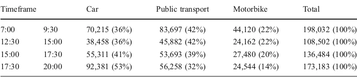
After the estimation phase, the whole model system has been implemented and applied to the Naples’metropolitan area. The application results for the City of Naples (just urban trips) are shown in Table8in terms of total trips per time-of-day and per mode, not explicitly distinguishing the effects of first and second tours. However, the going-to-work trips of the first tour actually determinate the total number of trips of the first timeframe; similarly, only (part of) the caming-back trips of the first tour contribute to the trips in the second timeframe. In all other timeframes the contributions of different tours are mixed and therefore the modal shares are some intemediate values between those characteristic of tour 1 and 2 reported in Table7.
In more detail, the morning peak-hour, 07:00–09:30, is characterized by about 200,000 work trips inside the city of
Timeframe Car Public transport Motorbike Total
7:00 9:30 70,215 (36%) 83,697 (42%) 44,120 (22%) 198,032 (100%) 12:30 15:00 38,458 (36%) 45,882 (42%) 24,162 (22%) 108,502 (100%) 15:00 17:30 55,311 (41%) 53,693 (39%) 27,480 (20%) 136,484 (100%) 17:30 20:00 92,381 (53%) 56,258 (32%) 24,544 (14%) 173,183 (100%) Table 8 Naples worker travel
demand by time-of-day and mode
Urban destination Extra-urban destination
Car Public transp. Motorbike tot Car Public transp. Motorbike Tot
tour 1 36.9% 41.8% 21.3% 100% 69.9% 27.1% 3.0% 100%
tour 2 67.4% 23.4% 9.2% 100% 87.4% 11.9% 0.8% 100%
Naples. In this timeframe the most frequently used mode is public transport, accounting for 84,000 trips (42% of the total); cars are chosen by more than 70,000 workers (35%); and the motorbike mode is used by more than 44,000 workers (22%).
In the off-peak timeframe, 12:30–15:00, the modal shares are the same as the morning peak-hours, as previously anticipated, with a worker demand level of about 110,000.
Between 15:00 and 17:30 more than 135,000 workers travel within the city of Naples. In this timeframe cars and public transport have the same modal share with about 55,000 workers per mode (about 40% of the total), while motorbikes are used by more than 27,000 workers (20%).
The 15:00–17:30 timeframe is the afternoon peak-hour; the Naples demand exceeds more than 170,000 workers; the most widely used mode is the car, with more than 92,000 trips (53% of the total); public transport is chosen by more than 56,000 workers (32% of the total), while motorbikes are used by about 25,000 workers (14%).
5 Conclusions
In this paper an activity-based modelling framework has been presented which tries to take into account the interaction among individuals participating to the same set of activities, as well as all temporal and physical constraints among single trips. The proposed framework allows to reproduce activity lists and activity patterns in an explicit and consistent way. As a consequence, time and mode characteristics of travel demand are more accurately computed.
In the paper a comprehensive formalisation of the modelling framework is presented and part of it is estimated on the basis of ad-hoc collected data. The modelling framework has been then applied to the Naples’ metropol-itan area.
The proposed framework has shown a satisfying flexibility, as well as a good ability in reproducing real data. It seems to be a good compromise between accuracy and operative issues, which improves the range of reproducible mobility phenom-ena and the accuracy of this reproduction and at the same time it moves some step forward the practical applicability of activity-based approaches.
Of course, the proposed approach presents an higher computational complexity with respect to more consolidat-ed trip or tour-basconsolidat-ed models, but the way it can be employed for transportation policy analyses and/or apprais-als is not different from traditional demand modeling approaches. It can be employed in order to obtain more realistic Origin/Destination modal matrices, as well as more realistic elasticity of these matrices to changes of network
levels of service. Assignment of these matrices to networks also allows for more realistic assessment of network and congestion effects of transportation policies.
Future research will mainly attempt to extend the model specification and estimation to the first three choice dimensions, related to the weekly household activity list formation and distribution among the days of the week and the individuals of the household. The proposed framework should also be applied to contexts different from that used for the estimation and the obtained results should be compared with those obtainable from other activity and non activity-based approaches, so as to highlight the introduced improvements. The hope of this paper is that of providing anyway an interesting contribution to the literature of this complex field by showing a possible comprehensive theoretical formulation of the problem and its applicability to a real context.
Open Access This article is distributed under the terms of the Creative Commons Attribution Noncommercial License which per-mits any noncommercial use, distribution, and reproduction in any medium, provided the original author(s) and source are credited.
References
1. Ruiter ER, Ben-Akiva M (1978) Disaggregate travel demand models for the San Francisco Bay Area. Transp Res Rec 673:121–128 2. Domencich T, McFadden D (1975) Urban travel demand: a
behavioural analysis. North-Holland, Netherland
3. Richards MG, Ben-Akiva M (1975) A disaggregate travel demand model. Lexington Books, USA
4. Horowitz J (1980) A utility maximizing model of the demand for multi-destination non-work travel. Transp Res B 14B:369–386 5. Adler T, Ben-Akiva M (1979) A theoretical and empirical model
of trip chaining behavior. Transp Res B 13:243–257
6. Gunn HF, van der Hoorn AIJM, Daly AJ (1987) Long range country-wide travel demand forecasts from models of individual choice, in Proc. Fifth International Conference on Travel Behaviour (Aiix-en Provence)
7. Hague Consulting Group (1992) The Netherlands National model 1990: the national model system for traffic and transport. Ministry of Transport and Public Works, Netherlands
8. Algers S, Daly A, Kjelmann P, Wildert S (1995) Stockholm model system (SISM): application. In Proc. Seventh World Conference of Transportation Research. Sydney, Australia
9. Cascetta E, Nuzzolo A, Velardi V (1993) A system of mathemat-ical models for the evaluation of integrated traffic planning and control policies, technical report Laboratorio Ricerche Gestione e Controllo Traffico. Salerno, Italia
10. Jones PM, Koppelman F, Orfeuil JP (1990) Activity analysis: state-of-the-art and future directions. In: Jones P (ed) Developments in dynamic and activity-based approaches to travel analysis. Gower, Aldershot 11. Ben-Akiva M, Lerman SR, Damm D, Jacobson J, Pitschke S,
Weisbrod G, Wolfe R (1980) Understanding, prediction and evaluation of transportation related consumer behaviour, Center for Transportation Studies, MIT. Cambridge, Massachussetts 12. Pas EI, Koppelman FS (1987) An examination of the determinants
13. Pas EI (1988) Weekly travel-activity behavior. Transportation 15:89–109
14. Meloni I, Cherchi E (1997) Activity based approach: un’ applica-zione alla generaapplica-zione degli spostamenti. In: Amoroso S, Crotti A (eds) Proc. Il Trasporto Pubblico nei Sistemi Urbani e Metropol-itani, vol 1. SIDT Collana Trasporti, Franco Angeli, Milano, pp 65–94
15. Cirillo C, Axhausen KW (2002) Mode choice of complex tours. In Proc. European Transport Conference. Cambridge, UK, September 16. Bhat CR, Guo JY, Srinivasan S, Sivakumar A (2004) A
comprehensive econometric micro-simulator for daily activity-travel patterns. Transp Res Rec 1894:57–66
17. Bowman JL, Ben-Akiva ME (2001) Activity-based disaggregate travel demand model system with activity schedules. Transp Res A 35:1–28 18. Townsend TA (1987) The effects of household characteristics on the multi-day time allocations and travel-activity patterns of households and their members, Ph.D. thesis, Northwestern University, Evanston, IL
19. Kitamura R (1988) An evaluation of activity-based travel analysis. Transportation 15:1–2
20. van Wissen LJ (1989) A model of household interactions in activity patterns. In Proc. International Conference on Dynamic Travel Behavior Analysis. Kyoto University, Kyoto, Japan, pp 16–17, July 21. Golob TF, McNally MG (1997) A model of activity participation and travel interactions between household heads. Transp Res B 31 (3):177–194
22. McNally MG (2000) The activity-based approach, Institute of Transportation Studies and Department of Civil & Environmental Engineering University of California, Irvine
23. Olaru D, Smith B (2005) Modelling behavioural rules for daily activity scheduling using fuzzy logic. Transportation 32 (4):423–441
24. Lee M, McNally MG (2006) An empirical investigation on the dynamic processes of activity scheduling and trip chaining. Transportation 33(6):553–565