Feeder Reconfiguration and Distributed Generator Placement in Electric Power Distribution Network

http://www.sciencepublishinggroup.com/j/ajece doi: 10.11648/j.ajece.20180202.16

ISSN: 2640-0480 (Print); ISSN: 2640-0502 (Online)

Feeder Reconfiguration and Distributed Generator

Placement in Electric Power Distribution Network

Pyone Lai Swe

Department of Electrical Power Engineering, Technological University (Yamethin), Mandalay, Myanmar

Email address:

To cite this article:

Pyone Lai Swe. Feeder Reconfiguration and Distributed Generator Placement in Electric Power Distribution Network. American Journal of Electrical and Computer Engineering. Vol. 2, No. 2, 2018, pp. 56-63. doi: 10.11648/j.ajece.20180202.16

Received: November 23, 2018; Accepted: December 13, 2018; Published: January 15, 2019

Abstract:

Power system deregulation and shortage of transmission capacities have led to an increase interest in Distributed Generations (DGs) sources. The optimal location of DGs in power systems is very important for obtaining their maximum potential benefits. A novel approach is proposed in this paper for placement of Distributed Generation (DG) units in reconfigured distribution system with the aim of reduction of real power losses while satisfying operating constraints. This paper presents an efficient method for feeder reconfiguration associated with DG allocation in radial distribution networks for active power compensation by reduction in real power losses and enhancement in voltage profile. Modified plant growth simulation algorithm has been applied successfully to minimize real power loss because it does not require barrier factors or cross over rates because the objectives and constraints are dealt separately. The main advantage of this algorithm is continuous guiding search along with changing objective function because power from distributed generation is continuously varying so this can be applied for real time applications with required modifications. The proposed system has been implemented with different scenarios on 33 bus Yamethin distribution system.

Keywords:

Feeder Reconfiguration, DG, Sensitivity Analysis, Radial Distribution System, Location and Sizing

1. Introduction

Distributed generation could be considered as one of the viable options to ease some of the problems (e.g. high loss, low reliability, poor power quality, congestion in transmission system) faced by the power systems, apart from meeting the energy demand of ever growing loads. Distributed generation (DG) devices can be strategically placed in power systems for grid reinforcement, reducing power losses and on-peak operating costs, improving voltage profiles and load factors, differing or eliminating for system upgrades, and improving system integrity, reliability, and efficiency. The aim of the DG placement is to provide the best locations and sizes of DGs to optimize electrical distribution network operation and planning taking into account DG capacity constraints. There are various types of DGU like solar Photovoltaic panels which can supply only real power at unity power factor. Some DGU can supply real as well as reactive power like solar thermal turbo alternators, biomass or biogas turbo-alternators, and wind turbines. There are many benefits of distributed generation like loss reduction, greener environment, and

improved utility of system, reliability, voltage support, and improved power quality, transmission and distribution capacity release. Distributed Generation plays an important role in electricity markets and power systems. Installation of DG on distribution feeders can have a significant impact on power system operation and control [1]. DG can be fitted with different strategies in the power network. For example, reducing power losses, cost reduction peak load, improving voltage profile or system reliability, all depend on the location and size of the DG [2]. Since selection of the best locations and sizes of DG units is also a complex combinatorial optimization problem, many methods are proposed in this area in the recent past [3]. Wang and Nehrir [4] proposed an analytical method to determine optimal location to place a DG in distribution system for power loss minimization. Celli et al. [5] presented a multi-objective algorithm using GA for sitting and sizing of DG in distribution system.

monitor and control the distribution networks as well as reconfiguring the distribution system to reduce the power losses and balance loads under normal operating conditions. Distribution networks have two types of switches, sectionalizing switches that are normally close and tie switches that are normally open. The distribution system has to operate in a way that the operating costs would be reduced as much as possible while the distribution system is supposed to remain radial, all loads should be provided, the transformers and lines should not be overloaded, and the voltage drop should remain within the permissible limit. Optimal network reconfiguration is, in fact, the best network configuration among all existing configurations in the network. Since distribution networks are configured in a radial manner, switches that are normally open or closed are strategic points of the network for reconfiguration. In general, reconfiguration to reduce power losses and eliminate overload or improve voltage profile in the network takes place which with the feeder load change and proper opening and closing of the switches can perform these actions [6]. Distribution network reconfiguration is a problem of complicated multi-objective integer combination optimization. The complexity of the problem arises from the fact that distribution network topology has to be radial and power flow constraints are nonlinear in nature [7]. Merlin and Back [8] proposed a heuristic algorithm to determine the minimum losses configuration. In this algorithm, all network switches are first closed to form a meshed network. The switches are then opened successively to restore radial configuration. Other heuristic algorithms were proposed by Civanlar et al. [9]. Artificial intelligence methods have also been applied to distribution network reconfiguration problems extensively, for example, genetic algorithms [10], neural networks [11], simulated annealing [12], swarm optimization [13], ant colonies [14]. In [3], authors have dealt with network reconfiguration and DG placement simultaneously using Harmony Search Algorithm (HSA) based only on minimization of power losses. In [15] using fireworks optimization algorithm for solving the distribution system network, reconfiguration, together with DG placement, for the problem of power loss minimization and voltage stability enhancement has been done.

The load as well as the generation varies with time continuously so an evolutionary algorithm which can deal with variations in load and generation is the Plant Growth Simulation Algorithm (PGSA) which is based on the plant growth process the root is the initial point of growth which is similar to initialization, then growth of the trunk and branches occur from nodes which is like searching for optimal values. Modification in evolutionary algorithms is done to make the convergence faster for making them suitable for real time applications. In this paper modification on the PGSA has been carried out and simulations are carried out to demonstrate the advantage of faster convergence of the proposed algorithm (MPGSA) over other algorithms for applications in DNR with and without DG. The main advantage of MPGSA is that constraints and objective function are dealt separately.

In this paper, optimal placement of DG using loss sensitivity factor method is proposed. The proposed approach has been demonstrated on 33 bus Yamethin distribution system. The rest of the paper is organized as follows: power loss using Network Reconfiguration and DG installation is presented in ‘Problem Formulation’ and ‘Grid System Scheme’. The achievement results and the related discussions are given in ‘Simulation Results’ and the paper ends in ‘Conclusion’.

2. Problem Formulation

2.1. Objective Function of Problem

The objective function of the problem is formulated so as to get maximum power loss reduction in distributed system which is the sum of power loss reduction due to reconfiguration as well as connection of DGU, which is subject to the voltage, current and power flow constraints as shown below:

max( _LossR _LossDG)

Maximize= ∆P + ∆P

Subjected V_min≤ V_k ≤V_max

, 1 , 1,max

k k k k

I ₊ ≤ I ₊

,

1 1

( )

n n

GK k Loss k

k k

P P P

= =

≤ +

∑

∑

(1)

2.2. Power Flow Equations

Power flows in a distributed system are calculated by using the following set of simplified recursive equations which are used to calculate the real and reactive power flows for finding the power losses

1 , , 1

k k Los k L k P₊ =P −P −P ₊

{

2

}

2 2

1 k₂ ( ) 1

k k k k k k Lk

k R

P P P Q Y V P

V

+ = − + + − +

The calculation of the power loss in line section connecting buses k and k+1 is given by

2 2

2

( , 1) k k

Loss k

k P Q

P k k R

V

 

+

 

+ = _{ }

 

 

(2)

The power loss of the feeder, PT,Loss may be calculated by

adding the losses of all line sections of the feeder, which is

,

1

( , 1)

N T Loss Loss

k

P P k k

=

=

∑

+ (3)

1 , , 1

{

2

}

2 2 2

1 ₂ 1

2

2 1 1

( )

k

k k k k k k k k

k

k k lk X

Q Q P Q Y V Y V

V

Y V Q

+ + + = − + + − − − (4) 2 2

2 2 2 2

1 ₂

2 2 ₂

2 2 2 2

2

2

( ) 2( )

( ) 2( )

2( ( ))

k k

k k k k k k k k

k

k k

k k k k k k

k

k k k k k k R X

V V P Q R P X Q

V

R X

V P Q Q Y V

V

R P X Q Y V

+ = − + + − +

+

= + − + − + −

+ +

(5)

2.3. Power Loss Using Feeder Reconfiguration

The use of reconfiguration in a radial distribution network is to identify a best configuration which can give a minimum power loss without violating the operation constraints. The operating constraints here are voltage limits, current capacity of the feeder feeding each and every bus always. The power loss of a line section connecting buses between k and k + 1 after the reconfiguration of network is calculated as

'2 '2

'

'2

( , 1) k k

Loss k

k P Q

P k k R

V   +   + = _{ }     (6)

Total power loss in all the feeder sections, P’T,Loss can be

found by adding up the losses in all line sections of the network. Which expressed as

' '

,

1

( , 1)

N

T Loss Loss k

P P k k

=

=

∑

+ (7)

The difference of power loss before and after reconfiguration (6)–(7) which is the Net power loss reduction, ∆PRLoss, is given as

'

, ,

1 1

( , 1) ( , 1)

N N

R

Loss T Loss T Loss

k k

P P k k P k k

= =

∆ =

∑

+ −

∑

+ (8)

2.4. Power Loss Reduction Using DG Installation

By connecting a distribution generation units in a radial distribution system at optimal locations give several advantages like reducing line losses, improving voltage profile, reducing peak demand reduction in overloading of distribution lines, reduction in environmental pollution and distribution systems.

The objective of DG placement problem is to minimize the real power losses of the distribution network through determining the optimal DG sizing and location. The operating constraints of the problem are divided into equality and inequality constraints.

For n bus radial distribution system, the problem is formulated as

2 min( DG Loss, )

Manimize f = W

Where

(

)

, 1 1 ( ) n n

DG Loss ij i j i j ij j i i j i j

W α P P Q Q β P Q PQ

= =   =

∑ ∑

_ + + − _ where

(

)

cos ij

ij i j

i j R

V V

α = δ δ− (9)

ij ij ij Z =R +X

(

)

sin

ij

ij i j

i j R

V V

β = δ δ−

Zij is the impedance of the line between bus i and bus j;

Rij is the resistance of the line between bus i and bus j;

Xij is the reactance of the line between bus i and bus j

Vi is the voltage magnitude at bus i;

Vj is the voltage magnitude at bus j;

δi is the voltage angle at bus i;

δj is the voltage angle at bus j;

Pi and Qi is the active and reactive power injection at bus i;

Pj and Qj is the active and reactive power injection at bus j

Subjected to: Equality Constraints:

The power flow equations must be satisfied as:

(

)

1

cos( ) sin( )

i DGi Di n

i j ij i j ij i j

j

P P P

V V G δ δ B δ δ

=

= −

=

∑

− + − (10)

(

)

1

sin( ) cos( )

i DGi Di n

i j ij i j ij i j

j

Q Q Q

V V G δ δ B δ δ

=

= −

=

∑

− + − (11)

Where, PDGi and QDGi are distributed power generations at

bus i. PDi and QDi are the loads at bus i. Gij is the conductance

of the line between bus i and bus j and Bij is the susceptance of

the line between bus i and bus j. Inequality Constraints:

Power generation limit must be satisfied as

min max

min max

DGi DGi DGi

DGi DGi DGi

P P P

Q Q Q

≤ ≤

≤ ≤ (12)

Bus Voltage limitVmin≤ ≤Vi Vmax Objective function

The objective function of the problem is to minimize the real power loss of radial distribution system under certain operating condition

Subjected to: (i₎ V_min ≤V_k ≤V_max

(ii_{) | |≤ ,}

(iii) Pi=PDGi--PDi & Qi= QDGi-QDi

(iv₎

min max

min max

DGi DGi DGi

DGi DGi DGi

P P P

Q Q Q

≤ ≤

≤ ≤

(v) System should be radial.

2.5. Identification of Loss Sensitivity Factor Method to Find Location of DG

To solve the DG allocation and sizing problem, sensitivity analysis method is used. The sensitivity factor of real power loss with respect to real power injection from DG is given by

,

1

2 ( )

n DG loss

i ij j ij j

i i

P

sf P Q

P ₌

α

β

∂

= = −

∂

∑

(13)

Computational procedure:

Step 1: Run load flow program for base case.

Step 2: Calculate the sensitivity factor using Eq. (13) of each bus and rank the sensitivity in descending order and form priority list.

Step 3: Select the bus which has highest priority and place DG at that bus.

Step 4: Now change the size of DG in ‘‘small’’ step and calculate real power loss for each size by running load flow program.

Step 5: Store the size of DG that gives the minimum loss. Step 6: Compare the loss with the previous solution. If loss is less than previous solution, store this new solution and discard previous solution.

Step 7: Repeat step 4 to 6 for all buses in the priority list.

3. Modified Plant Growth Simulation

Algorithm (MPGSA)

The plant growth simulation algorithm (PGSA) is based on the plant growth process, where a plant grows a trunk from its root; some branches will grow from the nodes on the trunk; and then some new branches will grow from the nodes on the branches. Such process is repeated, until a plant is formed. Based on an analogy with the plant growth process, an algorithm can be specified where the system to be optimized first ‘‘grows’’ beginning at the root of a plant and then ‘‘grows’’ branches continually until the optimal solution is found which has been used for Distribution Network Reconfiguration (DNR) but MPGSA gives result quickly when compared to PGSA for our simultaneous DG and reconfiguration and DNR requirement.

3.1. Probability Model of Plant Growth

A probability model for optimization is established based on the plant growth, in the node (Y) on a plant a function g(Y) has been introduced for describing the environment, If the

value of g(Y) is less the environment for growing a new branch is better. The algorithm is explained briefly as follows, the growth of the trunk is from its root B0. If here are k nodes

and BM1, BM2,..., BMK is having better environment than the

root B0 on the trunk M. If the function g(Y) of the nodes BM1,

BM2,..., BMK and B0 satisfies g(BMI) < g(Bo) then the

concentration of chemical morphactin responsible for plant growth CM1, CM2,..., CMK of the nodes BM1, BM2,..., BMK shall

be found by using the equation as followed the Equation (14).

0

1

( ) ( )

( 1, 2,..., )

Mi Mi

g B g B

C = − i= k

∆ (14)

1 0

1

( ( ) ( ))

k

Mi i

g B g B

=

∆ =

∑

−

The importance of Eq. (14) is that the morphactin a chemical mainly responsible for plant growth, its concentration in any node is based on the relative magnitude of the gap between the environmental functions between the root and the corresponding node in overall nodes, which actually describes the relationship between the concentration of chemical morphactin to environment which is the vital factor for growth of the plant and where branches will grow.

The morphactin concentrations can be derived as

1 1

M

C =

∑

, CM1, CM2,..., CMk of the nodes BM1, BM2,..., BMk

form a state space. The Selection of a random number β in between number [0, 1], is like throwing a ball in the interval which can drop into any one of CM1, CM2,..., CMk, then that

selected node called preferential node will take priority in the growth process for going a new branch in the next step. If random number β drops into CM2, which means

1 2

1 1

Mi Mi

i i

C

β

C

= =

≤ ≤

∑

∑

then the node BM2 will grow a new

branch m. If there are q nodes Bm1, Bm2,..., Bmq is the

environment of growth than morphactin concentrations are Cm1, Cm2,..., Cmq. The morphactin concentrations of the nodes

M has to be calculated for all nodes except for nodes where plant growth has already occurred due to which the concentration value becomes zero. The calculation can be carried out by summing up the related terms of the nodes on branch m and excluding the related terms of the node in which plant growth has already occurred. The main contribution of this paper lies in fixing a value for β as 0.5 which is based on number of trial and error combinations values tried between 0 to 1 so there is no random search for value of β which makes the algorithm faster and more suitable for real time application. So this algorithm is called as modified PGSA algorithm.

0

1 2

( ) ( )

( 1,3,..., )

Mi Mi

g B g B

C = − i= k

∆ + ∆

0

1 2

( ) ( )

( 1, 2,..., )

Mj Mj

g B g B

C = − i= q

( ) ( )

1 0

1 2

( )

k

Mi i i

g B g B

= ≠

∆ =

∑

−

( ) ( )

2 0

1

( )

q

Mi j

g B g B

=

∆ =

∑

−

The morphactin concentrations of all nodes will form a new state space except the one node which has already grown. The branch having highest morphactin concentration will grow in the next step and this repeats till plant is fully grown. The plant growth is modelled as follows the nodes of the plant is like solutions possible. The environment g(Y) function is like objective function. The length of trunk and branch is like possible search spaces. The initializing of the solution is the root of the plant. When the plant growth occurs in the branch having highest morphactin concentration called preferential growth is like searching optimal values. The growth node will form the initial value for next search operation. Thus the plant growth also called as plant photo tropism is used in solving optimization problem.

3.2. Implementation of Modified PGSA to Find the Optimal Power Loss with DG

Step 1: According to the priority list formed using sensitivity factor, place DG of different sizes at the chosen

bus.

Step 2: Calculate real power losses in the system using modified plant growth simulation algorithm (MPGSA) method for the selected values of DG.

Step 3: Compare the real power losses for every size of DGUs.

Step 4: Save the DG size corresponding to minimum real power loss.

Step 5: Continue Steps 2–4 for 50 iterations with 5 different sizes of DGU in every iterations (setting Nmax = 50).

Step 6: Choose the best size among 50 values with minimum real power loss and print the corresponding DGU.

4. Grid System Scheme

The base configuration of the system is having a single supply point with 33 buses, 3 lateral, 37 branches, 5 loops or tie switches (switches 33-37) which are kept normally open is shown in dotted lines which is closed only during fault condition to maintain continuity of supply or can be closed to change circuit resistance to reduce losses. The system has total load of 3.715 MW and 2.30 MVAR. The base network power loss is 202. 6762 kW and tie switches are 33, 34, 35, 36, 37. Figure 1 depicts the single line diagram of 33 bus Yamethin distribution system after applying feeder reconfiguration and DG placement at nominal load.

Figure 1. 33-bus Yamethin distribution system.

Assumptions and constraints

(1) Three small generators which are operated with a power factor of unity (i.e.) injecting only Real power is assumed for connection with the system in cases 3, 4, 5 solar photo voltaic system.

(2) The DG can be connected to any load bus based on loss Sensitivity factor.

(3) The capacity of DG sizes is limited upto 2 MW per bus. (4) The upper voltage limit is 1.05 p.u and lower voltage limit is 0.9 p.u

(5) Only one DG is allowed in each bus.

(6) The load model is used with a uniform constant power for simulation and voltage of primary bus is 1.0 p.u.

5. Simulation Result

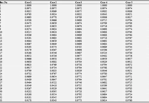
Table 1. Comparison Results of 33 Bus System.

Bus No. Case 1 Case 2 Case 3 Case 4 Case 5

1 1.0000 1.0000 1.0000 1.0000 1.0000

2 0.9971 0.9975 0.9972 0.9974 0.9974

3 0.9835 0.9869 0.9875 0.9882 0.9886

4 0.9763 0.9824 0.9832 0.9843 0.9851

5 0.9693 0.9778 0.9789 0.9806 0.9817

6 0.9508 0.9666 0.9680 0.9715 0.9784

7 0.9473 0.9659 0.9674 0.9709 0.9788

8 0.9337 0.9653 0.9678 0.9716 0.9793

9 0.9274 0.9624 0.9694 0.9698 0.9774

10 0.9215 0.9618 0.9691 0.9688 0.9763

11 0.9206 0.9684 0.9689 0.9688 0.9764

12 0.9191 0.9683 0.9682 0.9718 0.9767

13 0.9084 0.9659 0.9698 0.9692 0.9742

14 0.9067 0.9649 0.9699 0.9684 0.9734

15 0.9193 0.9574 0.9585 0.9689 0.9744

16 0.9179 0.9367 0.9696 0.9596 0.9737

17 0.9168 0.9546 0.9687 0.9524 0.9730

18 0.9052 0.9536 0.9677 0.9482 0.9756

19 0.9666 0.9958 0.9952 0.9959 0.9957

20 0.9630 0.9802 0.9784 0.9829 0.9912

21 0.9623 0.9769 0.9738 0.9794 0.9872

22 0.9917 0.9734 0.9704 0.9768 0.9738

23 0.9799 0.9833 0.9839 0.9846 0.9851

24 0.9732 0.9767 0.9774 0.9780 0.9784

25 0.9699 0.9654 0.9772 0.9647 0.9751

26 0.9489 0.9647 0.9764 0.9701 0.9729

27 0.9464 0.9522 0.9740 0.9682 0.9725

28 0.9349 0.9410 0.9735 0.9599 0.9733

29 0.9267 0.9329 0.9760 0.9641 0.9783

30 0.9232 0.9395 0.9728 0.9617 0.9763

31 0.9190 0.9354 0.9792 0.9604 0.9724

32 0.9181 0.9345 0.9787 0.9604 0.9759

33 0.9178 0.9343 0.9773 0.9614 0.9760

Table 2. Comparison Results.

Item Case 1 Case 2 Case 3 Case 4 Case 5

Real Power Loss (kW) 202.67 139.5 95.42 92.87 72.23

Vmin(p.u) 0.9052 0.9343 0.9585 0.9482 0.9724

Switches opened 33, 34, 35, 36, 37 7, 9, 14, 32, 37 33, 34, 35, 36, 37 7, 9, 13, 32, 37 7, 9, 13, 32, 37 Location of DG - - 17, 18, 33 31, 32, 33 18, 32, 33

Size of DG (MW) - -

0.1058 0.2469 0.6311

0.5900 0.1795 0.5568

1.0812 0.6645 0.5986

Table 3. Simulation Results of 33 bus Yamethin Distribution System.

Item Case 2 Case 3 Case 4 Case 5

DG placement - 17, 18, 33 31, 32, 33 18, 32, 33

DG size - 1.777 1.0909 1.7865

Open switches 7, 9, 14, 32, 37 33, 34, 35, 36, 37 7, 9, 13, 32, 37 7, 10, 14, 28, 31

Real power loss (kW) 139.5 95.42 92.87 72.23

% Real power loss 31.16 52.92 54.17 64.36

Vmin(p.u) 0.9343 0.9585 0.9482 0.9724

Case-1: The 33 bus radial distribution is without reconfiguration of feeders and without connection of distributed generators (Base case-scenario-1).

Case-2: The system in case-1 is reconfigured by opening/closing the sectionalizing and tie switches (Reconfiguration scenario-2).

Case-3: The same as case-1 but with a connection of 3 Nos. of DG units without reconfiguration (no reconfiguration but

only DG connection-scenario-3).

Case-4: Reconfiguration first then DG units are connected (two step operation of first reconfiguration of feeders next connecting DG units-scenario-4).

Tie switches 33, 34, 35, 36, 37 are opened and DG are placed at bus 17 (Latpankone Bus) (0.1058 MW), bus 18 (Inngone Bus) (0.590 MW) and bus 33 (Myinnar Bus) (1.0812 MW) in case 3. The opened switch is 7, 9, 13, 32, 37 and DG installation are bus 31 (Naungai Bus) (0.2469 MW, bus 32 (Theingone Bus) (0.1795 MW), bus 33 (Myinmar Bus) (0.6645 MW) in case 4. Tie switches 7, 14, 10, 28, 31 are opened and DG are placed at bus 18 (Inngone Bus) (0.6311 MW), bus 32 (Theingone Bus) (0.5568 MW) and bus 33 (Myinnar Bus) (0.5986 MW) in case 5. The lowest voltages and real power losses are 0.9585 p.u, 95.42 kW in case 3,

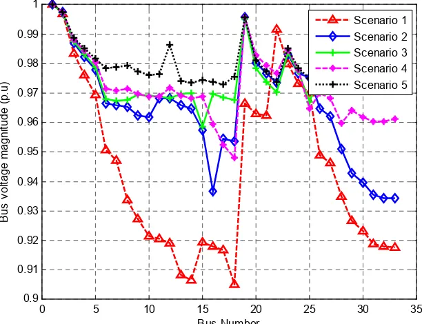
0.9482 p.u, 92.87 kW in case 4 and 0.9724 p.u, 72.23 kW in case 5. At the initial condition of the system, the total losses of the system are 202.67 kW. When three DGs are placed on the optimal location, the total losses of the system differ with respect to the original case. Table 1 and 2 and 3 show a better solution for voltage improvement as well as reduction in power loss. In the five cases compared for feeder reconfiguration with DG allocation gives least power loss with 72.23 kW which is for case 5 (scenario-5). The Figure 2 describes the voltage profile for all cases but case 5 shows a better voltage profile improvement out of all five cases.

Figure 2. Voltage profile of 33 bus system at five different cases.

When loads increase in 33 bus Yamethin distribution system, the scheme without considering feeder reconfiguration and DG placement cannot fulfill the load demand. Without feeder reconfiguration, the DG ability to support the system expansion with limited DG alternative sites. Therefore, it can be observed that feeder reconfiguration and DG placement are effective for loss minimization and voltage profile improvement.

6. Conclusion

Feeder reconfiguration transfers the load from the heavy-loaded feeder to the light one to balance the load distribution and postpone the system upgrade. Feeder reconfiguration does not need investment of new equipment, which can decrease the total planning cost especially with larger quality of tie-switches and section-switches. In this paper, the proposed approach for successful DG placement based on the sensitivity analysis, where the objective is to minimize the line losses and the bus voltage improvement is presented. The approach is performed on the 33 bus Yamethin distribution system. Results show that the proposed method is capable in determining the suitable location for DG. Moreover,

the optimal location DG in the system based on the sensitivity analysis can regulate the power flow of the system and can increase the voltages at each bus of the system and can reduce the power losses in the system. In this paper simultaneous reconfiguration and DG allocation for a 33 bus radial distribution system is proposed with a MPGSA algorithm. The results proves that the simultaneous reconfiguration with DG allocation give better results out of all other combinations. For this application of simultaneous reconfiguration and DG allocation the modified PGSA gives faster convergence. The proposed method and the results show that performance of proposed MPGSA is better and is more suitable for practical applications because the objectives and constraints are dealt separately.

References

[1] N. S. Rau and Y. H. Wan, “Optimal location of resources in distributed planning”, IEEE Trans. Power Syst., Vol. 9, pp. 2014-2020, Nov. 1994.

[2] W. EI-hattam, M. M. A. Salma, “Distributed GenerationTechnologies, Definitions and Benefits” Elect. Power Syst. Res., Vol. 71, pp. 119-1283, 2004.

0 5 10 15 20 25 30 35

0.9 0.91 0.92 0.93 0.94 0.95 0.96 0.97 0.98 0.99 1

Bus Number

B

u

s

v

o

lt

a

g

e

m

a

g

n

it

u

d

e

(

p

.u

)

[3] R. Srinivasa Rao, K. Ravindra, K. Satish, and S. V. L. Narasimham, “Power Loss Minimization in DistributionSystem Using Network Reconfiguration in the Presence ofDistributed Generation,” IEEE Trans. Power Syst., vol. 28, no. 1, pp. 317–325, Feb 2013.

[4] C. Wang and M. H. Nehrir, “Analytical approaches for optimal placement of distributed generation sources in power systems,” IEEE Trans. Power Syst., vol. 19, no. 4, pp. 2068–2076, Nov. 2004.

[5] G. Celli, E. Ghiani, S. Mocci, and F. Pilo, “A multi-objective evolutionary algorithm for the sizing and the sitting of distributed generation,” IEEE Trans. Power Syst., vol. 20, no. 2, pp. 750–757, May 2005.

[6] J. J. Young, K. J. Chul, Jin-O. Kim, J. O. Joong-Rin Shin, K. Y. Lee, An efficient simulated annealing algorithm for network reconfiguration in large-scale distribution systems, IEEE Trans. Power Del., vol. 17, no. 4, pp. 10 70–1078, October. 2002. [7] S. K. Goswami and S. K. Basu, “A new algorithm for the

reconfiguration of distribution feeders for loss minimization,” IEEE Trans. Power Del., vol. 7, no. 3, pp. 1484–1491, July 1992.

[8] A. Merlin and H. Back, “Search for a minimal-loss operating spanning tree configuration in an urban power distribution system,”in Proc. 5th Power System Computation Conf. (PSCC), Cambridge, U.K., pp. 1–18, 1975.

[9] S. Civanlar, J. Grainger, H. Yin, and S. Lee, “Distribution feeder reconfiguration for loss reduction,” IEEE Trans. Power Del., vol. 3, no. 3, pp. 1217–1223, Jul. 1988.

[10] K. Nara, A. Shiose, M. Kitagawa, and T. Ishihara, “Implementation of genetic algorithm for distribution systems loss minimum reconfiguration,” IEEE Trans. Power Syst., vol.7, no.3,pp.1044-1051,August 1992.

[11] H. Kim, Y. Ko, and K. H. Jung, “Artificial neural networks based feeder reconfiguration for loss reduction in distribution systems,” IEEE Trans. Power Del., vol. 8, no. 3, pp. 1356– 1366, July 1993.

[12] H. C. Chang and C. C. Kuo, “Network reconfiguration in distribution system is using simulated annealing,” Elect. Power Syst. Res., vol. 29, pp. 227–238, May 1994.

[13] J. Kennedy and R. Eberhart, “A discrete binary version of the particle swarm algorithm,” Proc. IEEE Int. Conf. on Systems, Man, and Cybernetics (SMC 97), vol. 5, pp. 4104–4109, October 1997.

[14] C. T. Su, C. F. Chang and J.-P. Chiou, “Distribution network reconfiguration for loss reduction by ant colony search algorithm,” Elect. Power Syst. Res., vol. 75, pp. 190–199, August 2005.

[15] A. Mohamed Imran, M. Kowsalya, D. P. Kothari “A novel integration technique for optimal network reconfiguration and distributed generation placement in power distribution network,” Electr Power Energy Syst., vol. 63, pp. 461–472, 2014.

[16] R. Srinivasa Rao, S. V. L. Narasimham, M. R. Raju, and A. Srinivasa Rao,“Optimal network reconfiguration of large-scale distribution system using harmony search algorithm,” IEEE Trans. Power Syst., vol. 26, no. 3, pp. 1080–1088, Aug. 2011. [17] H. R. Esmaeilian, R. Fadaeinedjad, “Energy Loss Minimization

in Distribution Systems Utilizing an Enhanced Reconfiguration Method Integrating Distributed Generation,” IEEE Syst. J., IEEE, pp. 1-10, July. 2014.

[18] N. G. A. Hemdana, B. Deppec, M. Pielked, M. Kurrata, T. Schmedesd, E. Wiebene “Optimal reconfiguration of radial MV networks with load profiles in the presence of renewable energy based decentralized generation” Elect. Power Syst. Res., Vol. 116, pp. 355-366, November 2014.

[19] M. E. Baran and F. Wu, “Network reconfiguration in distribution system for loss reduction and load balancing,” IEEE Trans. Power Del., vol. 4, no. 2, pp. 1401–1407, Apr. 1989.

[20] J. S. Savier and D. Das, “Impact of network reconfiguration on loss allocation of radial distribution systems,” IEEE Trans. Power Del., vol. 2, no. 4, pp. 2473–2480, Oct. 2007.