R E S E A R C H
Open Access
Incorporating shape constraints in
generalized additive modelling of the
height-diameter relationship for Norway
spruce
Natalya Pya
1*and Matthias Schmidt
2Abstract
Background: Measurements of tree heights and diameters are essential in forest assessment and modelling. Tree heights are used for estimating timber volume, site index and other important variables related to forest growth and yield, succession and carbon budget models. However, the diameter at breast height (dbh) can be more accurately obtained and at lower cost, than total tree height. Hence, generalized height-diameter (h-d) models that predict tree height from dbh, age and other covariates are needed. For a more flexible but biologically plausible estimation of covariate effects we use shape constrained generalized additive models as an extension of existing h-d model approaches. We use causal site parameters such as index of aridity to enhance the generality and causality of the models and to enable predictions under projected changeable climatic conditions.
Methods: We develop unconstrained generalized additive models (GAM) and shape constrained generalized additive models (SCAM) for investigating the possible effects of tree-specific parameters such as tree age, relative diameter at breast height, and site-specific parameters such as index of aridity and sum of daily mean temperature during vegetation period, on the h-d relationship of forests in Lower Saxony, Germany.
Results: Some of the derived effects, e.g. effects of age, index of aridity and sum of daily mean temperature have significantly non-linear pattern. The need for using SCAM results from the fact that some of the model effects show partially implausible patterns especially at the boundaries of data ranges. The derived model predicts monotonically increasing levels of tree height with increasing age and temperature sum and decreasing aridity and social rank of a tree within a stand. The definition of constraints leads only to marginal or minor decline in the model statistics like AIC. An observed structured spatial trend in tree height is modelled via 2-dimensional surface fitting.
Conclusions: We demonstrate that the SCAM approach allows optimal regression modelling flexibility similar to the standard GAM but with the additional possibility of defining specific constraints for the model effects. The
longitudinal character of the model allows for tree height imputation for the current status of forests but also for future tree height prediction.
Keywords: Height-diameter curve, Norway spruce, Shape constrained additive models, Impact of climate change, Varying coefficient models
*Correspondence: [email protected]
1Department of Mathematics, School of Science and Technology, Nazarbayev University, 53 Kabanbay Batyr Avenue, Astana, Kazakhstan
Full list of author information is available at the end of the article
Background
Two of the main questions of forest management planning concern the current status of forests and how forests will develop in future. To estimate forest stock and assortment from sample forest inventories, for example, in forest dis-tricts or federal states, single tree volumes have to be predicted and then summed up to get timber volume esti-mates for a considered forest area. A tree volume estimate is usually based on three parameters: tree species, tree diameter and tree height. Since measuring tree diameter at breast height (1.3 m) (dbh), is relatively cheap, but mea-suring tree height is cost intensive, it is desirable to model tree height as a function of tree species, tree diameter, tree age and other possible stand- and site-specific param-eters. An important feature of the height-diameter (h-d) relationship is that it develops over time and varies from stand to stand (Curtis 1967; Lappi 1997; Mehtätalo 2004). In Mehtätalo (2005) it is noted that trees reach matu-rity at different ages depending on site conditions. Hence, asymptotic height and the height that is reached at any particular age differ significantly among sites. The poorer the site conditions are, the lower the tree height will be for a certain age and dbh, with the dbh itself depending on age, stand and site conditions, but also on silvicultural treatments. Height of particular trees of a stand at prede-fined ages of usually 50 or 100 years is used as a measure for site quality and is denoted as ‘site index’.
In this paper we develop site-sensitive longitudinal h-d moh-dels for forests in Lower Saxony, Germany, with the main focus on modelling fixed effects via unconstrained (GAM) and shape constrained generalized additive mod-els (SCAM). Since climate change has already affected forests in Central Europe and much heavier impact is anticipated in the future, the models should be applica-ble for prediction of future tree height development and able to quantify the impact of climate change. Therefore, to achieve the necessary higher causality we use a combi-nation of causal and proxy site parameters as predictors.
Many studies of forest research have been devoted to model the height-diameter relationship (see, e.g., Jayaraman and Lappi 2001; Eerikäinen 2003; Mehtätalo 2004; Sharma and Parton 2007; Schmidt et al. 2011). Sev-eral approaches are now available for height predictions. Those studies differ in the type of underlying princi-pal h-d model used: linear (Lappi 1997; Eerikäinen 2003) or non-linear (Huang et al. 1992; Calama and Montero 2004; Castedo-Dorado et al. 2006; Sharma and Parton 2007). The principal h-d models also vary on how the model coefficients are being interpreted, which is espe-cially important if they are then modelled as smooth func-tions of predictors. The approaches differ also in terms of the specification of the model effects. The effects are either assumed to be strictly linear or allowed for non-linear patterns for which spline techniques are commonly
applied (e.g., Schmidt et al. 2011). Finally, there are dif-ferent procedures to account for spatial autocorrelation. This can be modelled via dummy fixed effects or uncor-related random effects on the level of territorial units and stands (Jayaraman and Lappi 2001), Kriging methods (Nanos et al. 2004), a Markov random field smoother for estimating correlated random effects on the level of territorial units, or 2-dimensional smooth terms of the geographic location of the stands or sample plots (Schmidt et al. 2011).
In this study a general underlying modelling approach of a reparameterized version of the Korf-function, that was developed by Lappi (1997) is used as the princi-pal model. The reason for using this model is that the model parameters considered there are less correlated and have biological meaning. Moreover, a heuristic fix-ation of the ‘non-linear’ parameters applied in this case linearizes the model, which makes the generalized addi-tive model approach reasonable to use for the estimation of the covariate effects on the original parameters. The model is then extended to include some tree-specific and site-specific variables. As some of the covariate effects are supposed to be monotone, a shape constrained addi-tive modelling (SCAM) approach (Pya and Wood 2015) is applied to account for influence of such variables as tree age, relative diameter at breast height and altitude among others, and also of site variables that will partially alter with expected climate change.
Data
The data analyzed here are observations from 23 145 sam-ple plots of 29 324 Norway spruce trees [Picea abies (L.) Karst.] and some site-specific variables from the first cycle of the state forest enterprise inventories (district sample plot inventories) conducted by the Lower Saxony forest planning agency. Norway spruce is the most common and by far the most economically important species in Europe. Lower Saxony is the second largest federal state of Germany and is located in the north-western part. Every year two or three state owned forest districts are invento-ried. The data come from inventories in the time interval 1996 – 2008. There are almost no consecutive inventories during this period (no longitudinal data), but all forest dis-tricts are inventoried, with the exception of a small area of the “Nationalpark Harz”.
Two types of covariates are considered: tree-specific and stand- and site-specific. The tree-specific variables are tree diameter at breast height (dbh), tree age (age) and relative diameter at breast height (rel.dbh). The relative diameter at breast height is calculated as
rel.dbh=dbh/mqd,
within all trees in a stand. A similar covariate is used by Eerikäinen (2003) who used the tree’sdbhin relation to thedbhof a stand’s dominant tree as predictor.
The second type of covariates, site-specific, can be differentiated into causal and proxy site variables. The proxy variables include altitude (alt), topex index (topex.sw), and geographic location, easting (east) and northing (north) in Gauß-Krüger coordinates refer-ring to the 3rd meridian. The topex index describes topographic exposure and terrain morphology in the South-West direction. It is calculated as a sum of topo-graphic exposure indices in the directions to the West, South-West and South using a distance limit of 250 meters (see, e.g., Scott and Mitchell 2005). A digital terrain model (DTM) with a resolution of 90 meters by 90 meters was used for topex calculation. A tree located on a summit is highly exposed resulting in a negative topex index. Positive topex indices belong to sites such as depressed areas or valleys rectangular-orientated in the direction of the topographic exposure. Topex indices of trees growing along the flat areas would be near zero. Since exposure to the South-West might result in drought stress, the topex index is used as a proxy for drought stress. Moreover, extra exposed sites will usually show a lower capacity of avail-able soil water due to higher percentage of rocks and lower depth to parent rock.
The additional causal site (climate) explanatory vari-ables are temperature sum of daily mean temperature during vegetation period (growing season) (temp.veg), and De Martonne’s aridity index (ari). The aridity index is a fraction of annual precipitation in millimetres over mean annual temperature in degrees Centigrade plus ten (P/(T+10)) (De Martonne 1926; Thornthwaite 1931). The aridity index is calculated for the entire year, since the precipitation during winter (non-growing season) could be partially stored by the soil. Temp.vegand ari are retrospective simulation means (Spekat et al. 2007) of the normal climate period 1961–1990 that were regional-ized from weather stations of the German weather service (DWD) using GAM with model effects for the geographic location and altitude. Table 1 summarizes the data under study.
Methods
A difficulty with the h-d relationship is that it is not con-stant but rather varies from stand to stand and develops over time (Lappi 1997; Mehtätalo 2004). In this paper we use an approach to modelling the longitudinal h-d rela-tionship proposed by Schmidt (2010) that combines the principal h-d-model of Lappi (1997) with (unconstrained) generalized additive model technology as a starting point. The development of the h-d model consists of three steps: 1) initial specification of the h-d relationship as a log-linear mixed model with random stand effects, 2) ‘a priori’
Table 1Characteristics of Norway spruce trees and site parameters from the first cycle of all state forest enterprise inventories in Lower Saxony. 29 324 Norway spruce trees from 23 145 sample plots were observed
Min 25 % qu. Median 75 % qu. Max
Tree height [m] 3.7 14.6 21.8 27 47.3
dbh [cm] 7 16.8 30.5 37.9 104
Tree age [years] 20 41 54 77 199
Altitude [m] 0 90 307 475.2 947
Sum of topographic exposure –84 560 –3108 1489 8135 89 208
indices [°×1000]
(DTM 90 m×90 m resolution)
Temperature sum during 833.6 1716.4 1996.6 2196.5 2456.8
the vegetation period [°C]
Aridity index 24.8 37 44.8 54.6 87.5
determination of non-linear model parameters, and 3) developing unconstrained and shape constrained general-ized additive models for investigating potential tree and site specific effects on the original parameters of the modified Korf function (Lappi 1997).
The initial steps, 1) and 2), of the model development are briefly described in the following subsection.
Initial model development
A data base for the whole of Germany was applied for this ‘a priori’ estimation of specific model parameters. As a starting point, the following height-diameter model known as the Korf function is used for the description of the relationship between tree height and diameter (Lappi 1997):
highly correlated, it is suggested to reparameterizedbhas follows (Lappi 1997):
xki= (dbhki+λ)
−C−(30+λ)−C
(10+λ)−C−(30+λ)−C . The model (1) can now be written as
log(μki)=Ak−Bkxki, (2)
whereAk andBk are not highly correlated and have bio-logical meanings.Akis the expected value of the log height of trees withdbh=30 cm for sample plotk; andBkis the expected value of the difference in the log(Hki)between trees of dbh = 30 cm and 10 cm for sample plot k. These interpretations are important since the parameters will be described as functions of additional tree, stand and site-level covariates in the second step of the model development.
The model (2) is linear with respect toAkandBk. Taking into consideration the random stand effect, these param-eters can be represented at the first stage asAk = A+
αk,Bk = B+βk, whereAandBrepresent fixed effects which have to be estimated;αk andβk are random stand level effects with zero means and constant variance. It may be noted that (2) is overparameterized. Moreover, a model of that specification cannot be linearized with respect to the parametersλandC. Therefore, it is suggested firstly to estimateλandC. These parameters were selected by testing a variety of combinations ofλandCwhen fitting a linear mixed model
log(μki)=A−Bxki+αk+βkxki,
The combination of the parameters with the lowest error variance wasλ = 7 andC = 1.225. There were no clear trends found inλandC over different mean stand age and the models were not very sensitive to the valueC.
Additive model for tree height
One of the model requirements is to predict actual and future tree heights of a forest stand. Since every stand has different characteristics, effects of site and stand variables should be incorporated into the h-d model in combina-tion with an age effect that describes the developmental stage of the trees within a stand. Since the proportion of structured and multi-aged stands in Lower-Saxony is con-stantly increasing we use single tree age as a covariate. The additional tree- and site-specific effects on the original parameters A and B of the Korf function that are partially sensitive to climate change, are assumed to be non-linear. Then, based on the principal h-d model
log(μki)=A−Bxki, (3)
where the mean tree height can be modelled as a function of tree age and additional tree and site parameters using GAM (Hastie and Tibshirani 1990; Wood 2006a)
Model h1: unconstrained additive model
log(μki) = α0+f1a(ageki)+f2a(rel.dbhki) +f3a(topex.swk)+f4a(temp.vegk) +f5a(arik)+f6a(eastk,northk) +p0b×xki+p1b×ageki×xki+p2b ×altk×xki, (4)
where xki is the re-parameterized dbh of tree i on sample plot k introduced at the initial step of the h-d model development, α0 is the model intercept,p0b, p1b and p2b are model coefficients. Hki is assumed to fol-low a Gaussian distribution. The model termsf1a–f5aare unknown smooth functions of the corresponding predic-tor variables. We also added a spatial smooth function
f6a(east,north)of easting and northing, since there is a spatial correlation in the residuals. This unconstrained model assumes a linear combination of the covariate effects and due to the log-link, the effects act multiplica-tive exponentially on tree height.
In the above mentioned case the effects of age and alti-tude on the slopeBof the h-d curve were assumed to be linear. Now, suppose that both predictors have non-linear effects onB. Then the following model may be considered:
Model h2: GAM with varying coefficients
log(μki) = α0+f1a(ageki)+f2a(rel.dbhki) +f3a(topex.swk)+f4a(temp.vegk) +f5a(arik)+f6a(eastk,northk) +p0b×xki+f1b(ageki)×xki+f2b(altk)
×xki, (5)
where the non-linear effects of age and altitude are rep-resented by the smooth functionsf1b(age)andf2b(alt). Model h2 is referred to as a ‘variable coefficient model’ (Hastie and Tibshirani 1993; Wood 2006a).
The drawback of modelling with GAM is that it may result in insufficiently smooth effects of the covariates. Moreover, it is biologically plausible to expect that the effects of such covariates asage,rel.dbh,topex.sw, temp.vegandarion the original parameter A will be monotone under the current growth conditions of Lower Saxony, which is not guaranteed for the GAM fit. There-fore, we propose to impose additional constraints on the univariate smooth terms by applying a SCAM approach (Pya and Wood 2015) described in the next subsection.
Modelling non-linear effects using SCAM
Model h3: shape constrained additive model
log(μki) = α0+m1a(ageki)+m2a(rel.dbhki) +m3a(topex.swk)+m4a(temp.vegk) +m5a(arik)+f6a(eastk,northk) +p0b×xki+p1b×ageki×xki+p2b ×altk×xki. (6)
To distinguish from unconstrained smooths, smooth terms under monotonicity constraints are denoted bymja. The effect ofage on the original parameter A in (3) is supposed to be increasing, since for any constant vector of model predictors, the level of the h-d curve, that is the expected log(Hki) of a tree with dbh = 30 cm, is assumed to be increasing with increasing age. The effect
of rel.dbh on the original parameter A is expected
to be monotone decreasing, since lower values of the rel.dbhcorrespond to a lower rank of a tree within a stand. Within the same stand a tree with a lower rank has on average a greater competition pressure compared to a tree with a higher rank. While struggling for the light, suppressed trees have to invest more into height than diameter growth. Hence, trees will be taller with the value of rel.dbh decreasing given fixed values of dbh,ageand the additional covariates. Trees with high values ofrel.dbhare dominant trees that are usually more exposed to the wind and consequently, they have to invest more into diameter than height growth for sta-bility reason. Therefore, given any fixed covariate vector tree height is assumed to decrease with increasing val-ues ofrel.dbh. The effect oftopex.swon the original parameter A should be monotone increasing, since an exposure to the South West might result in drought stress as it was explained previously. We assume a monotone increasing netto assimilation with increasingtemp.veg under the climatic conditions of Lower Saxony (if not limited by the deficit of other resources). The lower site indices of Norway spruce, that are partially observed on warmer sites of Lower Saxony, are, for instance, assumed to result from limited water and lower nutrient supply. The effect of temp.veg must not be confused with optimum curves that are observed under varying tem-perature values in experiments. Hence, no temtem-perature optimum is assumed to be present under the current cli-matic conditions of Lower Saxony. The effect ofarion the original parameter A is expected to increase with increasing humidity. The lower site indices of Norway spruce that are partially observed on very humid sites in higher altitudes of the uplands, are assumed to be a result of limited temperature sums. Hence,ariandtemp.veg are both assumed to have monotone increasing effects on the original parameter A, hence on the level of the h-d curve.
Next, we consider the shape constrained version of the variable coefficient model h2 as model h4.
Model h4: SCAM with varying coefficients
log(μki) = α0+m1a(ageki)+m2a(rel.dbhki) +m3a(topex.swk)+m4a(temp.vegk) +m5a(arik)+f6a(eastk,northk)
+p0b×xki+m1b(ageki)×xki+m2b(altk)
×xki, (7)
where the non-linear effects ofageandalton the slope B are represented by the smooth functions m1b(age) andm2b(alt). Increasing effects of both m1b(age)and
m2b(alt) on the h-d relationship are assumed in this model. It is well known that the slope of the h-d rela-tionship increases with the developmental stage of a stand (e.g., Mehtätalo 2004). In our investigation age serves as a covariate that describes the developmental stage of a stand. Therefore, when fitting a varying coefficient model for the age effect on B, it should be monotone increasing. However, the gradient of the actual tree heights that are predicted in applications is also affected by thedbh val-ues that are used to initialize the model. The direction of the monotonicity of effectm2b(alt)remains unspecified at this point and will be defined later based on the results of the unconstrained model variant. Moreover, for all the monotonicity constraints a validation of the assumptions will be conducted based on the corresponding uncon-strained model effects.
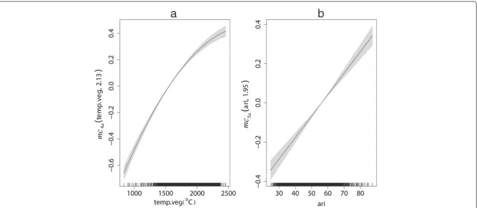
When fitting model with monotonicity constraints on the effects of temp.veg and ofari, we noticed some possibly artificial sharp changes in the corresponding esti-mated smooths (see sec. 4.2). To avoid these limitations the shape constrained model is enhanced by concavity constraints on the smooth terms of temp.veg and of ari. We propose model h5 as a variable coefficient model since the performance of model h4 was shown to be better than of model h3 in terms of AIC and GCV scores.
Model h5: SCAM with concavity constraints
log(μki) = α0+m1a(ageki)+m2a(rel.dbhki) +m3a(topex.swk)+mc4a(temp.vegk) +mc5a(arik)+f6a(eastk,northk) +p0b×xki+m1b(ageki)×xki+m2b(altk)
×xki, (8)
where now mc4a, mc5a are subject to both monotone increasing and concavity constraint.
Model h.ref:
log(μki) = α0+f1a(ageki)+p0b×xki+p1b ×ageki×xki. (9)
Model estimation
To estimate the SCAM models (6), (7) and (8) we employ the penalized regression spline approach which can be split into two stages: representation of smooth model terms via penalized unconstrained and constrained regression splines along with specification of the smooth-ness/wiggliness penalty followed by model coefficients estimation by penalized log likelihood maximization along with smoothness parameter selection by minimiza-tion of a predicminimiza-tion error criterion such as AIC or GCV. Shape COnstrained P-splines (SCOP-splines) (Pya and Wood 2015) were used for representation of the shape constrained smooth model terms. Since the bivariate function f6a(east,north) is a function of geographic coordinates, it was represented by a thin plate regression spline (Wood 2006a).
Combining the model matrices of each smooth column-wise into one model matrix and absorbing identifiabil-ity constraints result in the following expression of the SCAM model
log(μki)=Xkiβ, (10)
whereXis the combined model matrix of strictly paramet-ric model components and smooth basis functions and
βis a vector of unknown coefficients. After setting the penalties on each smooth model term which are expressed as quadratic forms of the full coefficient vector, β, the penalized log likelihood maximization can be written as
lp(β)=l(β)−βTSβ/2,
where l(β) is the log likelihood of the model, S =
kλkSk, andSkare the smooth penalty matrices enlarged by zeros to be expressed in terms of the full vector of the model coefficients,λkare smoothing parameters. The model coefficients, β, are estimated bylp(β) maximiza-tion given the values of the vector of smoothing parame-ters,λ. Optimization of thelp(β)is achieved by a Newton method which shares several features with a penalized iteratively re-weighted least squares scheme standard for GLM estimation. The smoothing parameter vector λ is estimated by minimizing the generalized cross validation score (GCV),
Vg=nD(βˆ)/(n−τ)2, whereD(βˆ) = 2
lmax−l(βˆ)
σ2is the model deviance, lmax is the saturated log likelihood,βˆ is the vector of the model parameters estimates, andτ is the effective degrees of freedom.
Confidence intervals for the model smooth terms are obtained through the distributional results for βˆ. The Bayesian approach to interval estimates for the smoothing spline models proposed by Wahba (1983) and Silverman (1985) was extended to generalized additive models by Lin and Zhang (1999) and Wood (2000). SCAM adopts this approach with an addition for establishing the approxi-mate distribution of the exponentiatedβ, denoted asβ˜, resulting in the normal distribution β˜|y ∼ N(βˆ˜,Vβ˜), where the expression for the covariance matrix Vβ˜ as well as all tedious details of the model parameters estima-tion can be found in Pya and Wood (2015). The SCAM approach is implemented in an R packagescamavailable at http://CRAN.R-project.org/.
To fit the unconstrained models h1 and h2 we use the penalized regression spline approach (Wood 2006a). The univariate functions f2a–f5a of (4) and (5) and also the unconstrained effectsf1bandf2bof model h2 (5) are rep-resented by P-splines (Eilers and Marx 1996) whereas an isotropic two dimensional thin plate regression spline (Wood 2006a) was used for representation of f6a. The standard penalized iteratively re-weighted least squares (PIRLS) scheme is applied for the model parameter esti-mation. The multiple smoothing parameter is selected by minimizing the GCV score in outer iterations. The Newton method is used for optimizing the GCV to update the smoothing parameter. The interval estimates for the component smooth functions of models h1 and h2 are obtained using the Bayesian approach to uncertainty esti-mation (Wahba 1983; Silverman 1985; Wood 2006b).
Results and discussion Model selection
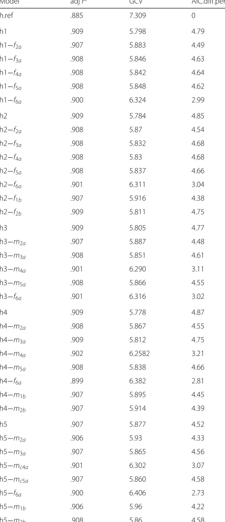
All covariates considered in the h-d models revealed their relevance to the tree height modelling. In addition we esti-mated possible submodels, where one at a time smooth effects were dropped. Table 2 presents the model fitting results (to keep the paper short, the results on the sub-models are shown only for the sub-models with one dropped smooth effect). The adjusted r2 and GCV scores are included into the table. The last column of the table shows the percentage of improvement in the Akaike information criterion (AIC.diff.perc) in comparison with the reference model, h.ref, calculated as follows
AIC.diff.perc= AICh.ref −AIChj AICh.ref ×
100,
Table 2Comparison of statistics for different
height-diameter-models including a base model with only age effects (h.ref), the unconstrained additive model (h1),
unconstrained additive model with varying coefficients (h2), shape constrained additive model (h3), shape constrained additive model with varying coefficients (h4), additive model with concavity constraints (h5). For all models the result of dropping single model effects on different model statistics are presented
Model adjr2 GCV AIC.diff.perc
h.ref .885 7.309 0
h1 .909 5.798 4.79
h1−f2a .907 5.883 4.49 h1−f3a .908 5.846 4.63 h1−f4a .908 5.842 4.64 h1−f5a .908 5.848 4.62 h1−f6a .900 6.324 2.99
h2 .909 5.784 4.85
h2−f2a .908 5.87 4.54 h2−f3a .908 5.832 4.68 h2−f4a .908 5.83 4.68 h2−f5a .908 5.837 4.66 h2−f6a .901 6.311 3.04 h2−f1b .907 5.916 4.38 h2−f2b .909 5.811 4.75
h3 .909 5.805 4.77
h3−m2a .907 5.887 4.48 h3−m3a .908 5.851 4.61 h3−m4a .901 6.290 3.11 h3−m5a .908 5.866 4.55 h3−f6a .901 6.316 3.02
h4 .909 5.778 4.87
h4−m2a .908 5.867 4.55 h4−m3a .909 5.812 4.75 h4−m4a .902 6.2582 3.21 h4−m5a .908 5.838 4.66 h4−f6a .899 6.382 2.81 h4−m1b .907 5.895 4.45 h4−m2b .907 5.914 4.39
h5 .907 5.877 4.52
h5−m2a .906 5.93 4.33 h5−m3a .907 5.865 4.56 h5−mc4a .901 6.302 3.07 h5−mc5a .907 5.860 4.58 h5−f6a .900 6.406 2.73 h5−m1b .906 5.96 4.22 h5−m2b .908 5.86 4.58
improves the unconstrained model h1, although to a lesser extent that it does in case of the SCAMs. Dropping either of the effects from any of the five considered models increases the AIC, with the exception of the three cases of the model h5 where the AIC slightly decreases. The other measures of the model performance such as the GCV and adjustedr2also give worse results than those of the full models h1-h5, when dropping any single effects. The spatial effect improves the model significantly: e.g., the models without spatial effect result in much higher GCV than the corresponding full model (about 24 % difference in the GCV in case of h2). Introducing stricter concavity constraints in model h5 leads to a slight increase in AIC and GCV, and correspondingly to a poorer model fit. It should be noted that there are only marginal differences in the performance criteria between the unconstrained GAM models h1 and h2, and their constrained coun-terparts, SCAM models h3-h5. The estimates and the corresponding standard errors of the coefficients of the linear part of the unconstrained model h1 and the shape constrained version h3 are shown in Table 3.
Interpretation of unconstrained effects and validation of their monotone counterparts
Overall, the monotonicity constraints on the univariate smooth terms result in less wiggly pattern compared to the unconstrained effects (see Fig. 2 versus Fig. 1). It should be noticed that the estimated effects of the shape constrained smooths are not centered as they are in the case of the unconstrained GAM, as different identifiability constraints were applied.
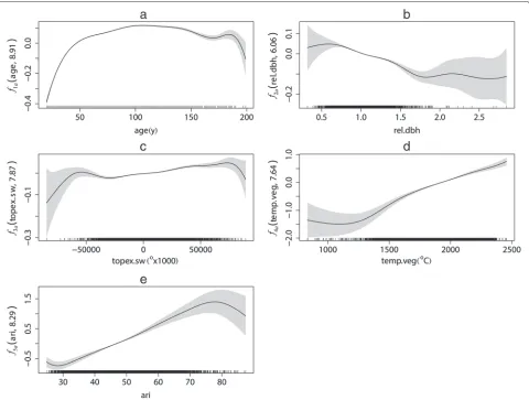
The estimated unconstrained effect ofageon the origi-nal parameter A of model h1 is increasing with a decreas-ing gradient for almost the whole data range (Fig. 1a). However, for high ages, above 150 years, the effect is implausibly decreasing. This pattern probably occurred due to an unbalanced data structure for the combination of site index and age. It is typical for forests and espe-cially managed forests that ‘old stands grow on poor sites’, since trees need longer production periods to reach mer-chantable timber dimensions. The proposed h-d models cover some site factors, e.g.temp.veg. However, a cer-tain proportion of the variability in site quality probably
Table 3Estimates of the coefficients of the linear parts of models h1 and h3. The corresponding standard errors are given in brackets
Model h1 Model h3
Intercept 3.095(.0011) -1.907(.399)
p0b .5654(.0084) .606(.0072)
p1b .00354(1.42×10⁻⁴) .00276(1.1×10⁻⁴)
Fig. 1The estimated smooth terms of the unconstrained model without varying coefficients, h1.athe smooth function of age, (b) the smooth function of relative diameter at breast height, (c) the smooth function of topex index, (d) the smooth function of temperature sum during the vegetation period and (e) the smooth function of aridity index. The labels of the vertical axes for the univariate smooths denote the smooth model components with the corresponding covariate and estimated degrees of freedom (edf) given in brackets
remains unquantified, which presumably leads to the implausible decreasing effect for high ages. The effect of ageof model h3 is assumed to be monotone increasing, so that at high ages the estimated smooth tends to a con-stant guaranteeing a plausible pattern over the whole data range (Fig. 2a).
The estimated unconstrained effect of rel.dbh of model h1 (Fig. 1b) supports the imposition of a mono-tone decreasing constraint on the functionf2a(rel.dbh) when constructing model h3. The confidence intervals of f2a near both boundaries of the data range are very wide which suggest that the minor deviates of the esti-mated smooth from monotonicity are not significant. The monotone effect of rel.dbh of model h3 is lin-ear with a negative slope which fulfills the imposed monotone decreasing constraint (Fig. 2b). The effect of
topex.sw on the original parameter A is not very
strong, which might be because the digital terrain model
used for the topex calculation has a low resolution of 90 m × 90 m (Fig. 1c). At the upper boundary of the range oftopex.swthe estimated smooth is considerably decreasing, but has a wide confidence interval. Hence, the assumption of a monotone increasing effect made in model h3 need not to be rejected. Although there is an increasing effect oftopex.swnear the lower boundary of the covariate range, this effect is much stronger (the gradient of the function is very steep) in comparison with the overall pattern. The corresponding confidence inter-vals are wide which might be due to the small amount of data available in that range. Therefore, the resulting lin-earity of the constraint effect could be validated as feasible also for this data range oftopex.sw. (Fig. 2c).
Fig. 2The estimated shape constrained univariate smooths of model h3.athe smooth of age, (b) the smooth of relative diameter at breast height, (c) the smooth of topex index, (d) the smooth of temperature sum during the vegetation period and (e) the smooth of aridity index. The labels of the vertical axes denote the smooth terms with the corresponding covariate and edf given in brackets
effect are mainly in accordance with findings of Albert and Schmidt (2009) who describe a monotone increasing effect with declining rate of mean temperature in growing season on site index for Norway spruce in Lower Saxony. In contradiction, Nothdurft et al. (2012) found an opti-mum curve with a slight tendency of a decreasing effect for high values of temperature sum in growing season for Norway spruce in Baden-Württemberg. This might be a result of the warmer climate of Baden-Württemberg which is located in Southwest Germany. However, an investigation for the whole of Germany (Schmidt 2010) showed monotone increasing effects of temperature sum in growing season and aridity index. These partially dif-fering results might be due to the collinearity of climatic covariates which hinders the estimation of robust causal effects especially for the upper boundaries of the data ranges. From our point of view the scam approach offers a possible solution to the problem by integrating expert knowledge. Even if the modelling procedure includes a more subjective component, we argue that predic-tions from our scam models are more reliable than their unconstrained counterparts, because of limited extreme
Fig. 3Model h5: the estimated smooth terms with both monotonicity and concavity constraints: (a) the smooth of temperature sum during the vegetation period and (b) the smooth of aridity index
in the gradient seems to be spurious. Figure 3 shows the estimated effects of the two terms with both mono-tone increasing and concavity constraints,mc4aandmc5a. This figure reveals now more convincing and reasonable smooth curves of the sum of daily mean temperature during vegetation period and aridity index. The other smooth terms of model h5 have similar effect to those of model h3.
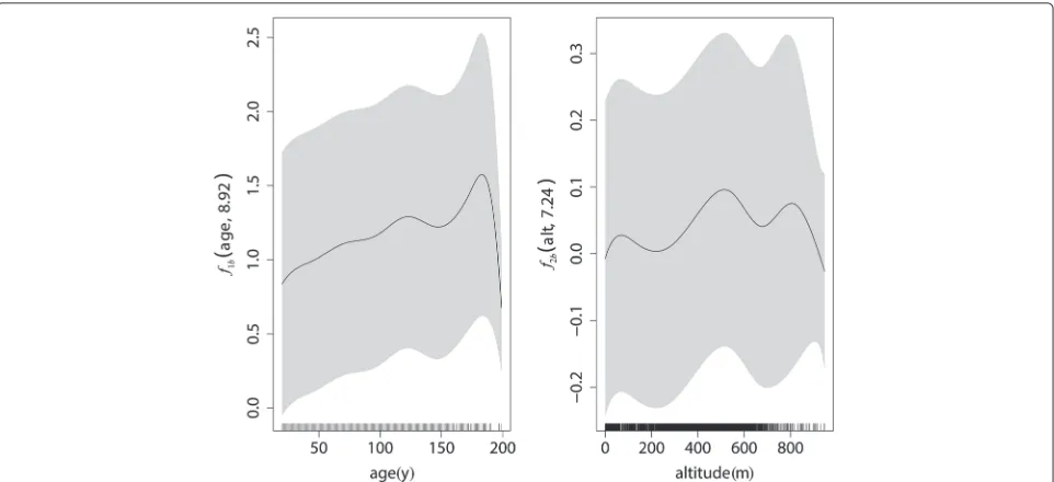
The estimated varying coefficients smooths of the unconstrained h2 and shape constrained h4 models, are illustrated in Figs. 4 and 5 correspondingly. From an expert view the unconstrained non-linear structure of the effects of age and altitude on the original parameter B is too flexible (Fig. 4). The unconstrained effect ofage sup-ports the assumption of an increasing slope of the h-d curve with increasing developmental stage, since gener-ally the effect ofageon B is increasing. Only for high ages the effect is decreasing. The unconstrained effect of alti-tude,f2b(alt), shows a weak increasing tendency, and the overall amplitude of the effect is small in comparison with the age effect. The corresponding confidence intervals are very large.
However, the two plots of the constrained version (Fig. 5) show the plausible monotone effects of age and altitude, although the non-linear structure of m2b(alt) is not very strong. Additional information about mono-tonicity of the effects narrowed the confidence intervals. The variability of the smooth estimates decreased as our beliefs in the shape of the effects were appended to the h-d relationship.
Figure 6 shows the spatial effect of the model h5. The effect was similar for the other considered models. The spatial smooth can be interpreted as a proxy of additional
predictors such as available water capacity of the soil, nutrient supply of the soil, etc., which were not at our disposal. The southern medium mountain area has better soil condition, therefore the trees are taller and slender in this part (light grey), compared to the worser conditions in the flat lands (silver) which have mainly glacial (sandy) type of soil. The conditions are even worse in terms of height growth near the North Sea coast (dark grey) due to the higher wind speed.
Conclusions
The presented framework and software allow the inclu-sion of a combination of shape constrained and uncon-strained smooth terms of one or more covariates as well as inclusion of strictly parametric model components and varying coefficient terms. The smoothing parameter selection is integrated with the SCAM parameter estima-tion procedure which is a great advantage. The model estimation scheme also provides interval estimates of the smooth terms which does not incur any additional simu-lations.
Fig. 4The estimated varying coefficients effects of the unconstrained model h2. Left panel: estimate off1b(age); right panel: off2b(alt). The labels of the vertical axes denote the smooth terms with the corresponding covariate and edf given in brackets
appropriate monotonicity constraints allows for an opti-mal combination of flexibility and expert knowledge to guarantee for a more robust modelling. This is especially useful in models using causal covariates applied to the prediction of future forest status.
The properties of the finally selected model (h5) can be summarized as follows:
1) The model comprises significant non-linear effects of covariates.
2) The plausibility of non-linear effects of covariates is enforced by the integration of monotonicity constraints.
3) The plausibility of some non-linear effects of
covariates is enforced by the additional integration of concavity constraints.
4) The implementation of expert knowledge via
constraints is enabled because the original parameters of the principal h-d model have a biological meaning.
Fig. 6An illustration of the non-linear effect of the spatial smooth
f6a(east,north)of model h5, all other covariates were set to their mean values. The coordinates are Gauß-Krüger coordinates referring to the 3rd Meridian. The black dots mark the locations of inventory plots and give an impression of the state owned forest area. Light grey indicates high values of log(E(Hki)), silver medium, and dark grey small values
5) The present autocorrelation in the large scale data base is covered by a 2-dimensional surface fitting as a function of coordinates.
6) The causality and generality of the model for prediction purposes is improved by use of causal site variables like sum of daily mean temperature during vegetation period and index of aridity.
None of the height-diameter-models referenced in the introduction chapter cover all these aspects simultane-ously. Most models assume linear effects of covariates (e.g., Lappi 1997; Eerikäinen 2003; Calama and Montero 2004; Mehtätalo 2004). However, sometimes transforma-tions of covariates are employed to achieve approximately linear effects (Eerikäinen 2003). At least in our case some of the estimated effects are significantly non-linear which would lead to biased predictions if disregarded. Moreover, there is a qualified need for constraining the non-linear effects because particularly at the boundaries of data ranges effect pattern resulted that conflict with expert knowledge. Hofner et al. (2011) presented a struc-tured additive regression model for ordered categori-cal data of the breeding distribution of Red Kite that employs monotonic penalized splines. As in our applica-tion they emphasize the optimal combinaapplica-tion of flexibil-ity and expert knowledge that is enabled by use of the
combined causal variables like a longtime mean cumula-tive temperature sum and a soil type classification with proxy site variables as we did. The advantage of proxy site variables is that they are usually known (like coordi-nates of stand centroids) or can be easily calculated with high accuracy (like altitude from high resolution digital terrain models). Causal site variables like continuous cli-matic and soil variables are usually unknown for forest stands or inventory plots and have to be predicted from auxiliary models. Thus they include a prediction error that will affect the height-diameter modelling also. How-ever, our decision to use causal site variables is based on the following reasons. 1) Our model should be able to predict future tree heights under projected changeable climatic conditions. 2) The integration of expert knowl-edge via monotonicity constraints is much more evident for causal covariates since proxy variables usually sub-sume several causal variables with differing effects. 3) The combination of causal covariates and monotonicity constraint improves the generality of the model in predictions.
The approach of SCOP-splines is an additional exten-sion of the variety of smoothing techniques incorporated in the R-library mgcv (Wood 2006a). For this specific application of modelling the height-diameter relationship of Norway spruce, we have shown that the implemen-tation of shape constrained smooths ensures a robust biologically meaningful interpretation with only marginal loss of prediction accuracy and no increase in prediction bias.
Competing interests
The authors declare that they have no competing interests.
Authors’ contributions
NP developed the R-packagescamthat was used for the model development. Both authors contributed to the model building, validation and writing of the manuscript. Both authors read and approved the final manuscript.
Acknowledgements
The forest data were provided by the Lower Saxony forest planning agency. NP has been partly funded by the EPSRC grant EP/K005251/1.
Author details
1Department of Mathematics, School of Science and Technology, Nazarbayev
University, 53 Kabanbay Batyr Avenue, Astana, Kazakhstan.2The Northwest German Forest Research Station, Department of Forest Growth, Grätzelstr. 2, 37079 Göttingen, Germany.
Received: 22 September 2015 Accepted: 28 January 2016
References
Albert M, Schmidt M (2009) Climate-sensitive modelling of site productivity relationships for Norway spruce (Picea abies (L.) Karst.) and common beech (Fagus sylvatica L.) For Ecol Manag 259:739–749
Brezger A, Lang S (2006) Generalized structured additive regression based on Bayesian P-splines. Comput Stat Data Anal 50(4):967–991
Calama R, Montero G (2004) Interregional nonlinear height-diameter model with random coefficients for stone pine in Spain. Can J For Res 34:150–163
Castedo-Dorado F, Diéguez-Aranda U, Barrio Anta M, Sánchez Rodríguez M, von Gadow K (2006) A generalized height-diameter model including random components for radiata pine plantations in northwestern Spain. For Ecol Manag 229(1-3):202–213
Curtis RO (1967) Height-diameter and height-diameter-age equations for second-growth douglas-fir. For Res 13(4):365–375
De Martonne E (1926) Une nouvelle fonction climatologique: l’indice d’aridité. La Météorologie (1942) 21:449–458
Eerikäinen K (2003) Predicting the height-diameter pattern of planted Pinus kesiya stands in Zambia and Zimbabwe. For Ecol Manag 175:355–366 Eilers PH, Marx BD (1996) Flexible smoothing with B-splines and penalties. Stat
Sci 11:89–121
Hastie T, Tibshirani R (1990) Generalized Additive Models. Chapman & Hall, Florida
Hastie T, Tibshirani R (1993) Varying-coefficient models. J R Stat Soc Ser B 55(4):757–796
Hofner B, Müller J, Hothorn T (2011) Monotonicity-constrained species distribution models. Ecology 92(10):1895–1901
Hökkä H (1997) Height-diameter curves with random intercepts and slopes for trees growing on drained peatlands. For Ecol Manag 97:63–72
Huang S, Price D, Titus SJ (2000) Development of ecoregion-based
height-diameter models for white spruce in boreal forests. For Ecol Manag 129:125–141
Huang S, Titus SJ, Wiens DP (1992) Comparison of nonlinear height-diameter functions for major Alberta tree species. Can J For Res 22:1297–1304 Jayaraman K, Lappi J (2001) Estimation of height-diameter curves through
multilevel models with special reference to even-aged teak stands. For Ecol Manag 142:155–162
Kammann EE, Wand MP (2003) Geoadditive models. J R Stat Soc Ser C 52:1–18 Kangas A, Maltamo M (2002) Anticipating the variance of predicted stand
volume and timber assortments with respect to stand characteristics and field measurements. Silva Fennica 36(4):799–811
Lappi J (1997) A longitudinal analysis of height/diameter curves. For Sci 43(4):555–570
Lin X, Zhang D (1999) Inference in generalized additive mixed models by using smoothing splines. J R Stat Soc Ser B 61:381–400
Mehtätalo L (2005) Height-diameter models for Scots pine and birch in Finland. Silva Fennica 39(1):55–66
Mehtätalo L (2004) A longitudinal height diameter model for norway spruce in finland. Can J For Res 34(1):131–140
Nanos N, Calama R, Montero G, Gil L (2004) Geostatistical prediction of height/diameter models. For Ecol Manag 195(1-2):221–235
Nothdurft A, Wolf T, Ringeler A, Böhner J, Saborowski J (2012) Spatio-temporal prediction of site index based on forest inventories and climate change scenarios. For Ecol Manag 279:97–111
Pya N, Wood SN (2015) Shape constrained additive models. Stat Comput 25(3):543–559
Schmidt M (2010) Ein standortsensitives, longitudinales Höhen-Durchmesser-Modell als eine Lösung für das Standort-Leistungs-Problem in
Deutschland. Deutscher Verband Forstlicher Forschungsanstalten Sektion Ertragskunde: Beiträge zur Jahrestagung 2010:131–152. http://
sektionertragskunde.fvabw.de/band2010/Tag2010_14.pdf Schmidt M, Kiviste A, Gadow K (2011) A spatially explicit height-diameter
model for Scots pine in Estonia. Eur J For Res 130:303–315
Scott R, Mitchell S (2005) Empirical modelling of windthrow risk in partially harvested stands using tree neighbourhood and stand attributes. For Ecol Manag 218:193–209
Sharma M, Parton J (2007) Height-diameter equations for boreal tree species in Ontario using a mixed-effects modeling approach. For Ecol Manag 249:187–198
Silverman BW (1985) Some aspects of the spline smoothing approach to nonparametric regression curve fitting. J R Stat Soc Ser B 47:1–52 Spekat A, Enke W, Kreienkamp F (2007) Neuentwicklung von regional hoc
Thornthwaite CW (1931) The climates of North America: according to a new classification. Geogr Rev 21(4):633–655
Wahba G (1983) Bayesian confidence intervals for the cross validated smoothing spline. J R Stat Soc Ser B 45:133–150
Wahba G (1990) Spline models for observational data. SIAM, Philadelphia Wood SN (2000) Modelling and smoothing parameter estimation with
multiple quadratic penalties. J R Stat Soc Ser B 62:413–428 Wood SN (2006a) Generalized Additive Models. An Introduction with R.
Chapman and Hall/CRC, Boca Raton, Florida
Wood, SN (2006b) On confidence intervals for generalized additive models based on penalized regression splines. Aust N Z J Stat 48(4):445–464
Submit your manuscript to a
journal and benefi t from:
7 Convenient online submission
7 Rigorous peer review
7 Immediate publication on acceptance
7 Open access: articles freely available online
7 High visibility within the fi eld
7 Retaining the copyright to your article