Species-specific, pan-European diameter increment models based on data of 2.3 million trees

R E S E A R C H

Open Access

Species-specific, pan-European diameter

increment models based on data of 2.3

million trees

Mart-Jan Schelhaas

, Geerten M Hengeveld

, Nanny Heidema

, Esther Thürig

, Brigitte Rohner

, Giorgio Vacchiano

,

Jordi Vayreda

, John Redmond

, Jaros

ł

aw Socha

, Jonas Fridman

, Stein Tomter

, Heino Polley

, Susana Barreiro

and Gert-Jan Nabuurs

Abstract

Background:Over the last decades, many forest simulators have been developed for the forests of individual European countries. The underlying growth models are usually based on national datasets of varying size, obtained from National Forest Inventories or from long-term research plots. Many of these models include country- and location-specific predictors, such as site quality indices that may aggregate climate, soil properties and topography effects. Consequently, it is not sensible to compare such models among countries, and it is often impossible to apply models outside the region or country they were developed for. However, there is a clear need for more generically applicable but still locally accurate and climate sensitive simulators at the European scale, which requires the development of models that are applicable across the European continent. The purpose of this study is to develop tree diameter increment models that are applicable at the European scale, but still locally accurate. We compiled and used a dataset of diameter increment observations of over 2.3 million trees from 10 National Forest Inventories in Europe and a set of 99 potential explanatory variables covering forest structure, weather, climate, soil and nutrient deposition.

Results:Diameter increment models are presented for 20 species/species groups. Selection of explanatory variables was done using a combination of forward and backward selection methods. The explained variance ranged from 10% to 53% depending on the species. Variables related to forest structure (basal area of the stand and relative size of the tree) contributed most to the explained variance, but environmental variables were important to account for spatial patterns. The type of environmental variables included differed greatly among species.

Conclusions:The presented diameter increment models are the first of their kind that are applicable at the European scale. This is an important step towards the development of a new generation of forest development simulators that can be applied at the European scale, but that are sensitive to variations in growing conditions and applicable to a wider range of management systems than before. This allows European scale but detailed analyses concerning topics like CO2sequestration, wood mobilisation, long term impact of management, etc.

Keywords:European forests, Diameter increment model, Climate change, Growth modelling, National forest inventory

* Correspondence:gert-jan.nabuurs@wur.nl

1_{Wageningen University and Research, Wageningen Environmental Research}

(WENR), Droevendaalsesteeg 3, 6708PB Wageningen, The Netherlands

14_{Wageningen University and Research, Forest Ecology and Forest}

Management Group, Droevendaalsesteeg 3, 6708PB, Wageningen, The Netherlands

Full list of author information is available at the end of the article

Background

The EU has a vision of sustainable forestry contributing to the economy of its Member States and to the envir-onment—both regionally and globally. In the latter con-text, the role of forests in biodiversity conservation and climate change mitigation as well as raw material provision has become increasingly important through the United Nations Convention on Biological Diversity (CBD) and the United Nations Framework Convention on Climate Change (UNFCCC). Forests in the EU’s 28 Member States stretch over a huge variety from the At-lantic in the west to the Black Sea in the east, and from the Mediterranean in the south to the boreal in the north covering 157 million ha (FOREST EUROPE2015). Forest management has evolved at a national or sub-national level influenced by the quantity and nature of the forest resources available, forecasts on their future development, perceived demand for raw material and services, and local economic and social factors. The management of forest resources has been affected in re-cent years by substantial shifts in the demands and ex-pectations put on forests, while the forest resource itself is subject to new pressures which are not yet sufficiently taken into account in national or international policies.

These pressures include diseases, invasive species, and the effects of climate change on forests through, e.g. drought, and storms (Lindner et al. 2014). Many forests continue to provide the traditional forest prod-ucts of timber, pulp, paper, etc., but forested areas are also expected to provide important ecosystem services, including climate change mitigation, conservation of bio-diversity, recreation and protection of water and soil (Nabuurs et al. 2006; Verkerk et al. 2011). A key policy issue is how the existing and future forests in the EU, which are limited in size and have a fragmented owner-ship, should be managed to deliver in a sustainable way an optimal mix of social, environmental (including biodiver-sity conservation) and economic services. These uncer-tainties plus a long planning horizon in forestry, require us to predict the long term impacts of management and environmental changes. One avenue is the employment of resource projection models (Barreiro et al.2017).

Making scenario projections of European forests is a hugely challenging task. Not only do they cover a large range of biotic and abiotic conditions, but they are spread over 46 countries, each with their own (forest) policies, inventory systems (Tomppo et al. 2010) and national forest resource projection systems (Barreiro et al. 2016; Barreiro et al. 2017). National forest in-ventory systems (NFIs), if existing at all, differ consider-ably in design, size thresholds, definitions, estimation methods, census interval, and importantly, in data access policy. A few countries have made their raw measure-ments available on the web (Netherlands, Germany,

France, Spain), a few make them available on request (e.g. Norway, Sweden), but still most results are only available in aggregated tables and reports. Even when the data are accessible, standardisation and harmonisation between NFIs remains difficult (Köhl et al.2000; McRoberts et al.

2009; Dunger et al. 2012). Data collection efforts like FOREST EUROPE (FOREST EUROPE 2015) and the Global Forest Resource Assessments by FAO (FAO2015) try to improve the harmonisation, but it remains a chal-lenge (COSTE432011). National forest resource projection systems show an even larger variety in design, methodolo-gies, processes and update cycles (Barreiro et al. 2016; Barreiro et al.2017), which makes it almost impossible to compare projections among countries.

Resource projections for Europe show different ap-proaches for handling the harmonisation challenge. For a long time, the European Timber Trend Studies (ETTS) as published by the UNECE/FAO were a collection of nationally executed projections of a set of standardised scenarios (Schelhaas et al. 2017). Nilsson et al. (1992) were the first to use a common, empirical projection tool applied country-wise on aggregated national forest inventory data. Since then, the same age-volume class matrix approach was developed and commonly applied as EFISCEN (European Forest Infor-mation Scenario model) in studies down to provincial resolution for the total European scale (Nabuurs et al.

2006; Schelhaas et al. 2015; Verkerk et al. 2016) for carbon balance studies, wood availability and e.g. trade-offs with biodiversity. Also, other models like CBM-CFS3 are being employed for European forest carbon balance assessments (Pilli et al.2016).

When the first European-scale forest resource models were developed, the approach chosen matched best with the predominant forest management approach in Europe (mostly even-aged management), the data availability (only aggregated data available), the issues to be addressed (large-scale resource availability, Member State level carbon sequestration) and the computing power available. In the meantime, the situation has chan-ged drastically. Forestry is now increasingly incorporating natural processes taking into account effects of climate change on growth (Peng2000) as well as the fulfilment of forest functions other than wood production (Verkerk

2015). As a consequence, the forests are becoming more heterogeneous in species and structure (Hector and Bagchi2007; Morin et al.2011; Zhang et al.2012), and a larger range of management options need to be consid-ered (Duncker et al.2012; Hengeveld et al.2012).

and usually based on NFI data (Barreiro et al. 2016), sometimes capable of incorporating anticipated future growth changes. These tools are usually not transferable to other countries because they are developed on very specific national conditions and datasets. However, a clear need can be identified for such simulation tools at the European level (Schelhaas et al. 2017). Such a tool should be able to 1) cover a wide range of biotic and abi-otic conditions, 2) have growth models sensitive to chan-ging environments, 3) be sensitive to varying forest systems and forest management approaches, and 4) be age-independent and have a high geographical detail. In this paper, we aim to develop a set of empirical individual-tree growth models that could be used in such a model at the European scale.

Methods

National forest inventory data

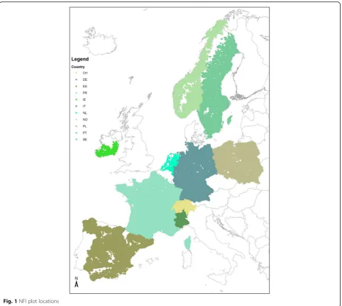
We collected individual tree measurements from avail-able National Forest Inventories to represent the range in growing conditions in Europe (Fig. 1). We included NFI data from Norway (Tomter et al. 2010), Sweden (Fridman et al. 2014), Netherlands (Schelhaas et al.

2014; Oldenburger and Schoonderwoerd 2016), Germany (Riedel et al.2016), a part of Ireland (Redmond

2016), Poland (Anonymous 2015), France (Hervé 2016), Switzerland (Lanz et al. 2016), Spain (Alberdi et al.

2016) and the Italian regions Piemonte (Camerano et al.

2008) and Aosta (Camerano et al. 2007). NFI systems differ in terms of inventory cycles, sampling system, plot radius, diameter threshold etc. (Table 1). Germany uses an angle count method (Bitterlich 1952), while other countries use a design with circular plots, either with a variable radius depending on the plot conditions, or with different radii with corresponding diameter thresholds. In total, observations were available for more than 2.3 million trees on over 190,000 plots, from 10 different NFIs. Except for France and the two Italian regions, data consisted of repeated tree diameter observations from permanent sample plots. Tree data included observation of diameter at breast height (DBH, hereafter simply referred to as diameter; all countries use a breast height of 1.3 m) during two consecutive measurements and identification of the tree species, for all trees that were alive both at the first and second observation.

In France, increment was recorded as the width of the last 5 tree rings as measured on a core, for all trees on the plot. In the two Italian regions, increment was avail-able as the 10-year radial increment of the tree closest to the plot centre, as measured on a core. Radial increment from tree core data was converted to diameter incre-ment (France, the two Italian regions). For these coun-tries we considered the measured diameter increment in the past as a prediction of the diameter increment in the

years after the observation, i.e. we did not reconstruct the diameter 5 or 10 years ago as starting point for the analysis. We chose this approach because plot basal area is one of the potential explanatory variables, and we didn’t have sufficient information to reconstruct plot basal area in the past. Tree circumference as measured in France was converted to diameter. All observations were converted to annual diameter increment by divid-ing the total diameter increment by the number of years between the measurements, using the YEARFRAC func-tion in Excel. Occasional observafunc-tions of negative diam-eter change were assumed to result from unbiased measurement errors, therefore these negative diameter changes were kept to avoid introducing bias.

We grouped the tree species in 20 species groups (Table 2). Minor species or species groups were itera-tively merged until sufficiently large groups remained. Species or species groups were retained if they cov-ered at least 5% of the total dataset over all countries, or if they were considered as an important species in a certain region of Europe, either in terms of production (like poplar plantations) or in coverage (likeQuercus ilex

(L.) andQuercus suber(L.) in the Mediterranean region). The group ‘Populus plantations’ includes only Populus

species and hybrids that are commonly used in commer-cial plantations while other Populusspecies are included in the category‘shortlived broadleaves’. For completeness in view of intended model application,‘rest’groups were created for broadleaves and conifers. For broadleaves the rest category was split into shortlived and longlived species based on authors’judgement.

Explanatory variables

We constructed a set of potential explanatory variables, covering information on the forest structure (F), soil (S), climate (C), weather (W) and nutrient deposition (D). Forest structure was represented by stand basal area at the time of first measurement as delivered by the differ-ent NFIs, and the variable F-rDiffDq, a proxy for the social position of each tree within the stand defined as:

FrDiffDq¼DBH=DBHq–1 ð1Þ

withDBHthe diameter of the tree and DBHq the quad-ratic mean diameter of all trees on the plot at the first observation. Values smaller than zero indicate that the tree is relatively small and more likely to be suppressed, while values larger than zero indicate that the tree is more likely to be dominant.

fraction, depth to bedrock, bulk density, cation exchange capacity (CEC), soil organic fraction and fraction of coarse fragments. The dataset consists of estimates of the respective properties at 7 depths ranging from 0 to 200 cm. We only used the third depth (15 cm), since the values at different depths were highly corre-lated. We also included a map with natural soil sus-ceptibility to compaction from the European Soil Data Centre (Panagos et al. 2012).

To derive climate characteristics, we used the World-Clim (Hijmans et al.2005) and the GEnS (Metzger et al.

2013, based on the WorldClim (Hijmans et al. 2005) and CGIAR-CSI data (Trabucco et al. 2008; Zomer et al.

2008)) datasets. Both datasets cover a range of climatic variables and indices (like monthly and annual means and extremes for temperature and precipitation, temperature and precipitation in coldest/warmest/wettest driest quarter

or summer/winter, several aridity and humidity indices, etc.), averaged for the period 1950–2000, at 1 km reso-lution. The datasets partly overlap but each set has some unique variables. Altitude correlates with weather and climate variables and is often included as predictor in simi-lar studies. However, the inclusion of altitude makes it impossible to include climate change effects directly in the model and thus we excluded it from the predictor set. For the same reason, latitude was not included either.

For nutrient deposition we used the EMEP data, con-taining deposition of oxidised and reduced nitrogen and oxidised sulphur at the 50 km grid (www.emep.int). Average nutrient deposition values were calculated for the period 1990–2010.

For weather, we obtained data from Agri4Cast (http:// agri4cast.jrc.ec.europa.eu/), at 25 km resolution for the period 1975–2015. We used this dataset to calculate a

range of weather indices (similar to the climate indices) for the actual observation period of each tree in our dataset. See Appendix 1 for more information on wea-ther indices and calculation procedures. In total we included 99 abiotic explanatory variables (for a full list see Appendix2).

To avoid simultaneous use of explanatory variables with large correlations in the models, we made a selec-tion among variables with correlaselec-tions greater than 0.8 or smaller than−0.8. This selection was based on scores that preferred simpler variables over more complicated ones (like average temperature over degree days above a certain threshold), weather variables over climate and easily available ones over those that are usually more dif-ficult to obtain. The full list of variables and their prior-ity in the data preparation is given in Appendix 2. Exclusion of correlated variables was done for each species group separately, since the spatial occurrence pattern of the species influences the observation range of the explanatory variables. Incomplete cases in the remaining dataset were removed.

Diameter increment model

Here, we restrict ourselves to modelling the diameter in-crement. Of all variables measured in the NFIs across

Europe, diameter is probably the most harmonised one, available for the largest number of trees, available as repeated observations on the same tree, and directly measured without further interpretation.

Some authors prefer to use basal area increment models over diameter increment models (Wykoff 1990; Quicke et al.1994; Monserud and Sterba1996; Schröder et al. 2002,) but Vanclay (1994) argues that both ap-proaches are essentially the same, since one can be de-rived from the other. Tree diameter generally develops according to an asymmetric sigmoidal function through time, with a slow, but rapidly increasing growth at estab-lishment, almost constant growth during the mature phase followed by a slow decline in growth during sen-escence (Tomé et al. 2006). Because creating new tree rings is essential for water transport, diameter increment will theoretically never reach zero, although the rings can be very small at old age.

Although age is known to be one of the best predictors of growth (Pukkala 1989; MacFarlane et al. 2002; Zhao et al. 2006; Tomé et al. 2006), we explicitly aim to ex-clude it as a predictor since it is not directly measured for all trees in the NFIs and forest situations in Eur-ope. Instead, we selected diameter, which is directly measured, as the predictor.

Table 1Overview of the NFI datasets used and their most important features

Country/Region Inventory cycle

Inventory dates Mean census interval (years)

Number of plots

Plot radius (m) Diameter threshold (cm) Comment NTrees

France NFI5–6 2005–2012 5 (core of all trees on the plot)

50,404 15 7.5 474,588

Germany NFI1/NFI2 1986−1989/ 2000–2002

14.3 10,344 angle count

method

137,425

Germany NFI2/NFI3 2002–2012 10.2 17,604 angle count

method

272,034

Italy - Piemonte 1999–2004 10 (core from 1 tree per plot)

13,192 variable (8-15 m)

7.5 DBH rounded

to cm

13,192

Italy - Aosta 1992–1994 10 (core from 1 tree per plot)

1691 variable (8-15 m)

7.5 DBH rounded

to cm

1691

Ireland NFI1/NFI2 2004–2006/ 2009–2012

6.1 577 3/7/12.62 7/12/20 8859

Netherlands NFI5/NFI6 2001–2005/ 2012–2013

9.5 1235 variable

(5–20 m)

5 18,348

Norway NFI9/NFI10 2004–2008/ 2009–2013

5 9243 8.92 5 201,484

Poland NFI1/NFI2 2005–2009/ 2010–2014

5 17,488 variable (7.98,

11.28 or 12.62)

7 350,487

Spain NFI2/NFI3 1986–1995/ 1996–2008

11.2 50,957 5/10/15/25 7.5/12.5/22.5/42.5 557,848

Sweden NFI7–8/ NFI8–9

2005–2009/ 2010–2014

5 14,833 3.5/10 4/10 246,852

Switzerland NFI2/NFI3 1993–1996/ 2004–2006

10.9 5217 8/12.6 (in flat

terrain)

12/36 DBH rounded

down to cm 49,192

Total 1986–2014 192,785 2,332,000

Modelling of sigmoidal relationships is usually achieved with so-called theoretical growth curves, such as the Lundqvist (Korf 1939; Stage 1963), Gompertz (Winsor 1932) and Chapman-Richards (Richards 1959) functions. Here, we choose the Gompertz function, be-cause it has the following properties:

1. The function is right-skewed, with a maximum growth at 1/e times the asymptotic diameter. 2. The derivative of the function with respect to time

(e.g. growth) can be written in a form only dependent on diameter.

Thus, for estimating diameter increment the derivative of the Gompertz equation is used:

dDBH

dt ¼β1DBHþβ2DBHlnDBHþε ð2Þ

with dDBH/dt the diameter increment (in mm), DBH

the diameter (in mm),β1and β2parameters andεis the error term with an assumed distributionN~(0,σ). These

parameters are a function of a set of independent vari-ablesXiexpressed as:

β1¼c1þ Xp

i¼1

θi;1Xi ð3Þ

β2¼c2þ Xp

i¼1

θi;2Xi ð4Þ

For both β1and β2 the variables Xi used to estimate

the parameter vectors are the same. The procedure for the selection of the p variables that best explain the diameter increment is described later. Values forcandθ are estimated using ordinary least squares (OLS) by substituting Eqs. 3 and 4 in Eq. 2.

The diameter when maximum growth occurs is de-fined by:

DBHopt ¼e

− β1

β2þ1

ð5Þ

with a maximum growth equal to: Table 2Summary of observed characteristics of the species after removing incomplete records

Reason for inclusion

Number of trees

Mean dbh (mm)

99th percentile DBH (mm)

Mean increment (mm∙yr−1)

Mean basal area (m2∙ha−1)

Mean mat (mean annual temperature) (degrees c)

Mat standard deviation

Mean tap (total annual precipitation) (mm∙yr−1₎

Tap standard deviation

Abiesspp. A 54,974 340 799 4.8 38.4 9.7 1.5 855 202

Larixspp. A 24,508 332 700 3.9 31.5 8.9 2.5 871 287

other conifers D 31,063 271 613 5.4 22.5 11.3 4.0 817 368

Picea abies A 373,235 248 635 3.6 34.5 7.1 2.8 836 273

Picea sitchensis B 8074 253 554 7.0 39.1 10.5 0.9 983 220

Pinus nigra + mugo C 66,237 239 579 2.9 21.7 12.1 1.7 500 189

Other indigenous pines C 204,443 268 580 4.0 20.5 13.6 2.4 563 305

Pinus sylvestris A 529,184 237 531 2.9 28.7 8.5 2.8 641 152

Pseudotsuga menziesii B 23,070 333 736 7.2 34.8 10.8 1.1 794 146

Betulaspp. A 149,484 145 414 1.8 21.4 5.9 3.6 752 220

longlived broadleaves D 199,048 223 673 2.9 25.3 11.3 2.0 726 201

shortlived broadleaves D 109,732 189 589 3.1 27.2 9.6 3.1 763 215

Castanea sativa C 34,812 287 1114 3.9 31.5 12.4 1.6 832 227

Eucalyptusspp. B 6770 273 678 7.9 18.7 15.2 1.3 1014 421

Fagus sylvatica A 163,123 331 807 3.6 33.0 10.1 1.5 791 176

Populusplantations B 2513 392 925 9.3 26.5 11.3 1.5 690 155

Quercus ilex C 68,173 237 764 1.8 12.2 14.3 2.1 536 156

Quercus robur + petraea A 179,861 335 827 3.3 28.7 10.9 1.6 778 204

Quercus suber C 20,616 319 796 2.3 16.6 16.3 1.4 640 161

Robinia pseudoacacia B 10,154 212 551 4.2 26.3 11.7 1.7 783 176

dDBH

dt max¼−β2DBHopt ð6Þ

The census interval in the datasets is overall either around 5 or 10 years depending on the country. To re-late the total diameter increment in this varying period to the diameter using a non-linear model, we use the average between the two measured diameters as a proxy for the diameter.

Figure 2 illustrates the shape of the growth model. A simultaneous increase of β1 and β2 by the same

percentage increases the maximum diameter incre-ment that can be reached, but leaves the diameter with maximum diameter increment and the maximum diameter unchanged. A small relative decrease of β1,

or the same relative increase in β2, lowers the curve

as a whole, resulting in smaller maximum diameter increment, a smaller diameter of maximum diameter increment and a smaller maximum diameter that can be reached.

Variable selection and model fitting

The selection of variables to be included in the model was performed in two phases for each species inde-pendently. First, a forward selection procedure was used. Given the large number of data points, the dataset was split in a selection-dataset (75%) and an acceptance-dataset (25%). Variables were added one-at-a-time. First, using the selection-dataset the add-itional variables were ranked based on the Akaike in-formation criterion (AIC, Akaike 1974). Because the large number of observations bias the AIC towards ever decreasing values with increasing numbers of variables, acceptance of the best ranking variable was subsequently based on an F-test performed on the predicted values for the acceptance-dataset (Zar

1996). The variables selected for 10 independent

data-splits were combined to obtain a list of candidate var-iables. Secondly, these candidate variables were used in a backward selection procedure on the full dataset for the final selection of explanatory variables. In this procedure the variable to be excluded was again se-lected based on AIC and it was actually excluded based on an F-test. The selected variables were used to estimate the full set of coefficients of the final model. The full models (substituting Eqs. 3 and 4 in Eq. 2) were fitted using OLS in the lm function in R (R:stats) (R core team 2014). For all F-tests a conser-vative α-value of 0.0001 was used to avoid overfitting the data. The average observed diameter increment was used as reference for calculation of F-tests and

R2*, rather than a reference value of 0 as is default when no intercept is included in the model. Model residuals showed some heteroscedasticity at small di-ameters (Additional file 1), but seemed homoscedastic over a large range of observations. We did not trans-form our data, which would introduce bias due to the need to exclude negative observations. In view of the intended model application we also calculated the R2*

of the total predicted basal area increment at plot-level for all available plots, including all species.

Results

The number of explanatory variables included in the final diameter increment models ranged between 2 and 25 for all species/species groups (Tables 3 and 4). Vari-ables of forest structure were always included (Table 4), weather and climate were included for 18 species, while soil and nutrient deposition were included for 16 and 13 species, respectively. R2* ranged from 0.10 for Quercus ilexto 0.53 for other conifers (Table4). TheR2*for total basal area increment at the plot level was 0.85. Conifers generally had greaterR2*than broadleaves (conifers 0.32 on average over all species and broadleaves 0.22). There was no clear relationship between the number of variables or variable groups selected and the explained variance. We tested the contribution to the explained variance of each group of variables by fitting the full model again, excluding the variables from that group, and recorded the decrease in R2*. If forest structural variables were left out from the model, the explained variance decreased by 43.9%, on average over all species groups. If weather variables were left out, the explained variance decreased by 8.7% and for climate by 3.8%. Soil and nutrient deposition accounted for respectively 2.2% and 1.4% of the explained variance. The weather variables most often selected were generally related to an-nual temperature (W-MaT), temperature variations (anan-nual temperature range W-aTR, mean diurnal range W-MaDR) or radiation (W-TaR), while less frequently selected vari-ables tended to include indices and minima and maxima

Table 3Selected variables and parameter estimates per species group. For abbreviations of variables see Appendix2

Abiesspp. Larixspp. Picea abies Picea sitchensis

θi,1 θi,2 θi,1 θi,2 θi,1 θi,2 θi,1 θi,2

c 6.65E–01 –1.13E–01 3.58E–01 −5.34E–02 −1.80E + 00 2.94E–01 5.13E–01 −7.59E–02

X1 F-lnBA −6.10E–02 9.12E–03 F-BA 9.60E–04 −1.59E–04 F-lnBA −5.07E–02 7.70E–03 F-BA −1.79E–03 2.88E–04

X2 F-rDiffDq 1.36E–02 −2.07E–03 F-lnBA −8.61E–02 1.37E–02 F-rDiffDq 5.90E–03 −9.13E–04 F-lnBA −3.90E–02 5.65E–03

X3 W-MaT 3.35E–03 −4.90E–04 W–MaT 3.77E–03 −5.82E–04 W-MaT 6.34E–04 −5.79E–05 F-rDiffDq 6.23E–02 −9.29E–03

X4 W-TaR 1.15E–06 −8.65E–07 W-TaR −3.61E–05 5.11E–06 W-TaP 1.87E–06 −6.67E–08 W-aTR −1.10E–02 1.67E–03

X5 W-aTR −2.83E–03 4.20E–04 W-SDmR 2.85E–04 −3.92E–05 W-aTR 3.06E–04 −6.98E–05 W-MweqR 2.21E–04 −3.50E–05

X6 W-SDmR 2.33E–05 3.22E–06 W-MweqR 4.46E–05 −7.37E–06 W-MweqT 8.21E–04 −1.26E–04 C-TwaqP −5.48E–04 8.90E–05

X7 W-MwaqP 3.56E–04 −5.39E–05 C-TaAET 1.12E–04 −1.74E–05 C-TaP 3.30E–05 −5.56E–06

X8 C-MaT −1.62E–04 2.97E–05 C-seaP 2.76E–04 −3.87E–05 C-ISO 1.52E–03 −1.58E–04

X9 C-TaP −9.37E–05 1.31E–05 S-PHIHOX −4.41E–04 5.31E–05 C-MaDR −7.93E–04 9.44E–05

X10 C-TaAET 1.29E–04 −2.03E–05 D-DepRedN −2.30E–05 3.89E–06 C-seaPET −5.91E–06 1.50E–06

X11 C-MaDR −8.56E–05 2.38E–05 D-DepOxN −2.65E–05 3.80E–06 C-Ari −1.43E–06 2.26E–07

X12 C-seaP −9.66E–04 1.34E–04 C-MwamT 6.73E–04 −1.10E–04

X13 C-MwemP 2.15E–04 −2.19E–05 C-MweqT −5.30E–05 7.78E–06

X14 C-MweqT −8.95E–05 1.21E–05 S-BLD 6.77E–05 −1.06E–05

X15 S-BLD 1.46E–05 −1.69E–06 S-BDRICM 9.98E–05 −1.25E–05

X16 S-CRFVOL −4.75E–04 6.38E–05

X17 S-BDRICM 3.34E–04 −4.84E–05

X18 D-DepOxN −1.63E–05 1.84E–06

X19 D-DepOxS 2.41E–06 −2.49E–07

Pseudotsuga menziesii Pinus nigra + mugo Other indigenous pines Pinus sylvestris

θi,1 θi,2 θi,1 θi,2 θi,1 θi,2 θi,1 θi,2

c 2.44E + 00 −3.70E–01 5.86E–01 −9.12E–02 5.36E–01 −8.42E–02 2.45E + 00 −3.76E–01

X1 F-lnBA −8.26E–02 1.23E–02 F-BA −1.90E–04 2.24E–05 F-BA −9.62E–04 1.60E–04 F-BA −1.34E–04 1.75E–05

X2 F-rDiffDq 6.35E–02 −9.66E–03 F-lnBA −3.09E–02 5.06E–03 F-lnBA −2.10E–02 3.05E–03 F-lnBA −4.77E–02 7.73E–03

X3 C-MaT −7.39E–04 1.13E–04 W-TaP −1.49E–05 3.03E–06 F-rDiffDq −5.77E–03 1.17E–03 F-rDiffDq 1.62E–02 −2.39E–03

X4 C-TaAET 4.11E–05 −5.45E–06 W-aTR −4.02E–03 5.98E–04 W-MaT 6.00E–03 −8.98E–04 W-MaT −1.21E–03 2.18E–04

X5 S-CRFVOL 7.72E–04 −1.19E–04 W-MINmPET −2.45E–03 3.83E–04 W-TaR 3.82E–06 −1.02E–06 W-TaP −1.44E–05 2.94E–06

X6 W-MdrqT 1.51E–03 −2.18E–04 W-aTR −3.38E–03 5.52E–04 W-aTR −3.17E–04 4.57E–06

X7 W-MweqR −1.56E–04 2.43E–05 W-MINmPET −1.76E–03 2.60E–04 W-ARi −1.32E–03 −3.32E–04

X8 C-seaT −2.33E–05 3.56E–06 W-MweqT −4.60E–03 7.38E–04 W-SDmP 4.43E–04 −6.87E–05

X9 C-ISO 9.18E–04 −1.28E–04 W-MweqR −4.05E–06 −8.03E–07 W-MINmP −5.34E–04 8.22E–05

X10 C-MweqT −1.30E–04 2.08E–05 C-TaPET 4.84E–05 −6.69E–06 W-McoqP 7.19E–05 −8.80E–06

X11 S-PHIHOX −1.47E–03 2.23E–04 C-seaP −8.93E–04 1.62E–04 C-TaAET 1.57E–04 −2.47E–05

X12 S-ORCDRC −4.82E–04 7.43E–05 C-MweqT −3.15E–04 5.12E–05 C-MaDR −5.63E–04 6.90E–05

X13 D-DepRedN −1.87E–05 3.11E–06 S-SLTPPT −5.94E–04 1.32E–04 C-seaP −3.60E–04 6.77E–05

X14 S-CEC 1.40E–03 −2.57E–04 C-seaPET 2.81E–05 −3.97E–06

X15 S-PHIHOX −4.49E–03 7.25E–04 C-ThARi 1.61E–03 −2.61E–04

X16 S-ORCDRC −7.32E–04 1.23E–04 C-MwamT −8.09E–04 1.25E–04

X17 S-CRFVOL −8.61E–04 1.34E–04 C-MweqT 7.75E–05 −1.22E–05

X18 D-DepOxN 5.93E–05 −9.84E–06 C-TwaqP 2.14E–05 −5.36E–06

X19 D-DepOxS −1.20E–05 2.21E–06 S-CLYPPT 1.18E–03 −2.04E–04

X20 S-CEC −7.36E–04 1.25E–04

X21 S-PHIHOX −1.88E–03 2.98E–04

Table 3Selected variables and parameter estimates per species group. For abbreviations of variables see Appendix2(Continued)

X23 S-BDRICM 0.000117916 −1.93E–05

X24 D-DepRedN 8.31E–07 −5.66E–08

X25 D-DepOxN 7.32E–06 −1.28E–06

Other conifers Betulaspp. Broadleaves longlived Broadleaves shortlived

θi,1 θi,2 θi,1 θi,2 θi,1 θi,2 θi,1 θi,2

c 4.28E–01 −6.48E–02 −2.87E–01 4.87E–02 2.71E–01 −4.01E–02 1.13E–01 −2.10E–02

X1 F-BA −3.18E–03 4.79E–04 F-BA −1.09E–03 2.00E–04 F-lnBA −2.66E–02 4.05E–03 F-lnBA −3.18E–02 4.67E–03

X2 F-rDiffDq 1.85E–02 −2.77E–03 F-lnBA −1.04E–02 9.42E–04 W-MaT 2.07E–03 −2.77E–04 W-aTR 3.23E–03 −6.25E–04

X3 W-MaT −3.23E–03 1.03E–03 F-rDiffDq 5.70E–03 −6.83E–04 W-TaR −1.67E–05 2.41E–06 W-SDmPET −1.93E–03 3.08E–04

X4 W-TaR −2.88E–05 2.75E–06 W-MaT 2.28E–03 −3.14E–04 W-aTR −4.52E–03 6.69E–04 W-SDmR 2.28E–04 −3.25E–05

X5 W-MaDR 7.36E–03 −1.12E–03 W-aTR 2.75E–03 −4.86E–04 W-ISO −6.38E–02 8.32E–03 C-TaP 9.83E–05 −1.79E–05

X6 W-ThHUi 1.21E–04 −1.29E–05 W-MaDR 1.65E–03 −2.93E–04 C-aTR 3.11E–04 −5.04E–05 C-TaAET −2.38E–05 6.85E–06

X7 W-SDmR −1.82E–03 3.01E–04 W-ARi −5.58E–03 7.71E–04 C-seaPET −9.14E–06 1.63E–06 C-ARi −5.32E–06 9.86E–07

X8 W-MweqT 8.80E–03 −1.67E–03 W-SDmPET −6.57E–04 8.35E–05 C-MweqT −7.00E–05 1.12E–05 C-MaDR 1.83E–04 −4.53E–05

X9 W-MweqR −2.44E–04 4.53E–05 W-SDmR 2.19E–04 −2.80E–05 S-CLYPPT −1.31E–03 2.04E–04 C-seaP −5.17E–04 7.30E–05

X10 C-MaDR 8.02E–04 −1.36E–04 C-seaP −6.96E–04 1.18E–04 S-SLTPPT 9.24E–04 −1.37E–04 C-seaPET −1.17E–05 2.87E–06

X11 C-seaP 2.54E–03 −3.87E–04 C-ThARi 2.16E–03 −3.50E–04 S-CEC −6.14E–04 9.11E–05 C-ThARi 5.40E–04 −8.44E–05

X12 C-MweqT −3.90E–04 5.05E–05 C-Tmm0P 8.94E–05 −1.52E–05 S-CRFVOL −7.39E–04 1.16E–04 S-CEC −9.07E–04 1.40E–04

X13 D-DepOxN 1.54E–04 −2.29E–05 C-TwaqP 2.64E–04 −3.95E–05 S-BDRICM 4.46E–05 −6.12E–06 S-PHIHOX −1.59E–04 5.27E–05

X14 S-SLTPPT 3.34E–04 −5.11E–05 D-DepRedN 1.79E–05 −2.57E–06 S-BLD 2.72E–05 −4.41E–06

X15 S-BLD 1.08E–04 −1.75E–05 S-CRFVOL −3.40E–04 3.71E–05

X16 S-BDRICM 1.87E–04 −2.29E–05

X17 D-DepRedN 8.21E–06 −1.15E–06

X18 D-DepOxN −2.70E–05 4.28E–06

Castanea sativa Eucalyptusspp. Fagus sylvatica Populusplantations

θi,1 θi,2 θi,1 θi,2 θi,1 θi,2 θi,1 θi,2

c 9.71E–01 −1.12E–01 −7.62E–01 4.22E–02 −4.53E–01 4.85E–02 5.08E–01 −7.29E–02

X1 F-BA 7.11E–04 −1.11E–04 F-BA −1.67E–03 2.46E–04 F-BA 6.27E–04 −9.59E–05 F-lnBA −6.96E–02 1.03E–02

X2 F-lnBA −6.26E–02 9.43E–03 F-lnBA −3.55E–02 5.21E–03 F-lnBA −5.56E–02 8.38E–03 W-aTR −9.81E–03 1.43E–03

X3 F-rDiffDq −1.09E–02 1.50E–03 F-rDiffDq −1.23E–02 8.33E–04 W-TaR −1.10E–05 1.70E–06

X4 W-ISO −7.33E–02 1.14E–02 W-MaT 1.53E–02 −2.88E–03 W-ISO −1.23E–01 1.78E–02

X5 W-MINmP 5.37E–04 −9.91E–05 W-TaP 5.78E–05 −9.31E–06 W-MaDR 4.24E–03 −5.96E–04

X6 C-MwamT −2.61E–04 2.78E–05 W-TaR −7.71E–05 1.18E–05 W-ThHUi 6.90E–06 8.34E–08

X7 C-TcoqP 1.04E–04 −1.45E–05 C-Ti 1.26E–04 −9.33E–06 W-ThARi 2.69E–04 −4.46E–05

X8 S-BLD 3.53E–05 −5.17E–06 S-SLTPPT −3.43E–04 1.38E–04 W-SDmPET −4.54E–04 5.58E–05

X9 S-CRFVOL −6.68E–04 9.19E–05 W-MweqT 9.60E–04 −1.40E–04

X10 D-DepRedN 2.63E–05 −3.67E–06 W-MdrqT −3.73E–04 5.33E–05

X11 C-MaT −2.74E–05 1.04E–05

X12 C-ISO 1.82E–03 −2.89E–04

X13 C-MINwamT 2.56E–04 −3.76E–05

X14 S-CLYPPT −6.78E–04 1.05E–04

X15 S-SLTPPT −5.87E–04 9.68E–05

X16 S-BLD 3.47E–05 −5.01E–06

X17 S-BDRICM 6.87E–05 −9.11E–06

X18 D-DepRedN 5.09E–06 −7.16E–07

Table 3Selected variables and parameter estimates per species group. For abbreviations of variables see Appendix2(Continued)

Quercus ilex Quercus robur + petraea Quercus suber Robinia pseudoacacia

θi,1 θi,2 θi,1 θi,2 θi,1 θi,2 θi,1 θi,2

c 1.72E–01 −2.68E–02 2.05E–01 −3.61E–02 1.09E + 00 −1.88E–01 2.24E–01 −3.30E–02

X1 F-lnBA −8.96E–03 1.30E–03 F-BA 1.05E–03 −1.58E–04 F-lnBA −1.39E–02 2.02E–03 F-lnBA −4.99E–02 7.51E–03

X2 F-rDiffDq −2.11E–02 3.10E–03 F-lnBA −5.93E–02 8.93E–03 F-rDiffDq −2.70E–02 3.89E–03 W-SDmP 3.35E–04 −4.12E–05

X3 W-MaDR −2.12E–03 3.51E–04 F-rDiffDq 1.01E–03 −1.20E–05 C-MaT −3.61E–04 6.31E–05

X4 W-MINmPET −4.56E–04 6.33E–05 W-TaR −7.46E–06 8.98E–07 S-comp 7.19E–03 −1.11E–03

X5 C-ISO −1.60E–03 2.72E–04 W-MINmPET 1.18E–04 −8.25E–06 D-DepOxS 3.67E–06 −4.94E–07

X6 C-TaP −6.10E–06 1.25E–06 C-TaPET 5.44E–05 −8.34E–06

X7 S-PHIHOX −3.17E–04 4.18E–05 C-seaP 4.16E–04 −6.10E–05

X8 D-DepOxN −1.33E–05 3.20E–06 C-MwamT −3.02E–05 7.03E–06

X9 S-CEC −8.33E–04 1.17E–04

X10 S-BLD 2.80E–05 −4.04E–06

X11 S-CRFVOL −4.36E–04 5.94E–05

X12 S-BDRICM 2.34E–04 −3.72E–05

X13 D-DepOxN 4.34E–06 −5.10E–07

Table 4First column: Number of variables selected per species group andR2*for the full model. Following columns: Number of variables selected per variable group in the final model, and the relative decrease inR2*_{if this variable group is omitted from the}

model and fitted again

Total Forest structure Weather Climate Soil Deposition

N R2_{* N R}2_{* relative}

decrease

N R2_{* relative}

decrease

N R2_{* relative}

decrease

N R2_{* relative}

decrease

N R2_{* relative}

decrease

Abiesspp. 19 0.29 2 32.3% 5 6.2% 7 3.3% 3 2.8% 2 0.7%

Larixspp. 11 0.28 2 60.7% 4 29.9% 2 2.0% 1 1.2% 2 3.3%

Picea abies 15 0.29 2 37.4% 4 0.6% 7 3.4% 2 0.9% 0 0.0%

Picea sitchensis 6 0.32 3 46.4% 2 13.0% 1 2.2% 0 0.0% 0 0.0%

Pseudotsuga menziesii 5 0.37 2 65.7% 0 0.0% 2 1.2% 1 0.2% 0 0.0%

Pinus nigra + mugo 13 0.33 2 28.3% 5 15.9% 3 3.7% 2 1.4% 1 0.3%

Other indigenous pines 19 0.26 3 32.2% 6 12.5% 3 3.5% 5 6.2% 2 1.1%

Pinus sylvestris 25 0.17 3 73.3% 7 3.7% 8 13.8% 5 4.0% 2 0.1%

Other conifers 13 0.53 2 16.5% 7 12.2% 3 3.9% 0 0.0% 1 3.0%

Betulaspp. 15 0.27 3 27.1% 6 1.9% 4 2.8% 2 2.0% 0 0.0%

Broadleaves longlived 14 0.2 1 28.0% 4 13.1% 3 1.3% 5 4.1% 1 2.8%

Broadleaves shortlived 18 0.25 1 25.1% 3 1.7% 7 5.8% 5 3.3% 2 0.5%

Castanea sativa 10 0.13 3 76.5% 2 5.2% 2 16.1% 2 5.1% 1 6.7%

Eucalyptusspp. 8 0.51 3 17.4% 3 23.5% 1 1.2% 1 0.9% 0 0.0%

Fagus sylvatica 19 0.25 2 27.9% 8 6.0% 3 3.1% 4 2.4% 2 0.3%

Populusplantations 2 0.2 1 73.5% 1 14.3% 0 0.0% 0 0.0% 0 0.0%

Quercus ilex 8 0.1 2 47.4% 2 8.0% 2 3.6% 1 1.3% 1 6.3%

Quercus robur + petraea 13 0.17 3 51.2% 2 1.8% 3 2.6% 4 5.4% 1 0.4%

Quercus suber 5 0.1 2 42.5% 0 0.0% 1 2.7% 1 2.5% 1 1.6%

for specific 3-month periods (quarters), related to precipita-tion and potential evapotranspiraprecipita-tion (PET). For the cli-mate variables no clear pattern could be distinguished, but also here annual variables were more often selected than in-dices and values for specific quarters.

To get an impression of the spatial variability in pre-dicted diameter increment, we calculated the growth of a tree for all locations where a tree of that species was present in our dataset. We assumed the tree had a diam-eter equal to the average diamdiam-eter of the species in the full dataset (Table 2), an F-rDiffDq of 0 (i.e. the social position of the tree was neutral) and that it was growing in a stand with a basal area equal to the average basal area listed in Table 2. We used the weather conditions of the period 2000–2014. Species groups show distin-ctively different spatial growth patterns (Fig. 3; Additional file2). Some species, likeFagus sylvaticaand

Abies spp., have slow growth at their southern distribu-tion limit and show good growth towards their northern limit, while other species like Picea abies show the

opposite pattern. Many species (Picea abies,P. sitchensis,

Populus plantations) show an east-west gradient with better growth along the coast and less growth going east, but Pseudotsuga menziesii and Quercus robur+petraea

show the opposite tendency. Only few groups (Pinus syl-vestris,Betulaspp.) show an optimum in their mid-range and decreased growth towards their distribution limits.

To illustrate the sensitivity of the final models we show the predicted diameter increment for a range of conditions (Fig. 4; Additional file 3). The main curve depicts the median diameter increment as predicted for all sites assuming the median F-BA and a neutral social position (F-rDiffDq = 0). Ranges depict devia-tions from this median growth for 5th and 95th per-centile of increment predicted for all locations, 5th and 95th percentile of F-BA observed in all locations and 5th and 95th percentile of F-rDiffDq observed in all locations. Additional file 4 shows the distribution of the underlying data and the moving average curves of both data and predictions.

Discussion

Growth of trees is governed by physical processes, plant physiological processes and ecological processes (Muys et al. 2010; Sterck et al. 2010). We have established a general description of the predicted diameter increment of European tree species as a function of the diameter and the biotic and abiotic environment of the tree. Even with the rather crude estimates of weather, climate, soil and nutrient deposition that were used, the strict shape of the growth curve, and the exclusion of the known good predictors age, latitude and altitude, we were able to explain between 10% and 53% of the variation in diameter growth of individual trees of the main European tree species and species groups. This level of explained variation is in line with the values reported by other studies based on country-scale forest inventory data-sets (e.g. Andreassen and Tomter2003; Laubhann et al.

2009; Cienciala et al. 2016; Charru et al.2017). Much of the unexplained variance seems to be attributable to within-stand variation, given the highR2*value for total basal area increment at the plot level given in the results section. Further application of the models should give insight in the predictive value at larger scales. Other studies (e.g. Laubhann et al. 2009) already applied regression models on individual-tree measurements for multiple European countries, but these studies were aimed at estimating effect sizes, rather than for predictive pur-poses. To our knowledge our study is the first to present tree diameter increment models with a European-wide validity.

Apart from the regular measurement errors within an NFI (McRoberts et al. 1994), our dataset may contain extra variability by mixing different NFIs with different designs, measurement methods, protocols and thresh-olds (Table 1). On first screening of the data, we could

not find indications for systematic differences between data from different NFIs, probably because we used the original diameter measurements without any further processing or interpretation. Additional noise is caused by the inclusion of explanatory variables of varying resolution (1–25 km), making it impossible to detect small-scale variation as present for example in moun-tainous terrain. However, the presented models are de-signed to be applied on a broad scale for large sets of plots, which will result in averaging out such errors. For studies on smaller scales, local or national diameter increment models might be better suited.

The largest part of the explained variance in the final models is attributed to parameters related to the forest structure, where basal area of the stand seems to be more important than the relative size of the tree (Fig.4; Additional file3). This is in line with many other studies that found stand density (Cienciala et al. 2016) or basal area (Hökkä et al. 1997) to be important variables. Des-pite the relatively low contribution of other variable groups to the explained variance, they are important to explain spatial patterns of diameter increment over Europe (Fig. 3; Additional file2). The spatial patterns of diameter increment as presented in Additional file 2

seem plausible. Picea abies and Picea sitchensis are known to grow well under wet conditions and moderate temperatures. At higher latitudes and altitudes, growth of Picea abiesis limited by a short growing season and low average temperatures, as indicated by declining diameter increment. For Picea abies a similar gradual decline is not visible on the southern edge. This is prob-ably because trees are killed by attacks of bark beetles after drought or heat waves (Seidl et al. 2007). The opposite pattern is found in Fagus sylvatica. At the southern edge, increment slows down as temperatures

rise, while there is an abrupt halt at the northern edge. This may be caused by mortality due to cold winters, or because Fagus is still expanding its range north-wards (Kramer et al. 2010). Pinus sylvestris is known for its wide ability to survive in a wide range of en-vironmental conditions. This is reflected in the spatial growth pattern with a large distribution over Europe, a moderate to good growth over a large range and declining growth only in harsh environments, such as dry inland Spain and under boreal conditions. Application of the models under climate change scenarios should give more information on the sensitivity of these patterns to climate change.

The diameter increment models presented allow for more detailed and consistent modelling of tree-growth at the European scale. With these models such modelling can take into account differences and changes in weather, climate and soil conditions across the continent and over time. As shown in Additional file 3, the models give realistic predictions over a large range of conditions. We recommend to use the models not further than the 99th percentile of diam-eter, as indicated in Table 2. Beyond these values the data support is very sparse, and the models may give unreasonable results. Similarly, the user should be aware that the models may predict small negative diameter increments for some species for specific combi-nations of poor locations, small diameters and high basal areas. The development of diameter increment models is a first step towards a full simulation model of forest devel-opment at the European scale. Such a growth model should include a way to estimate individual-tree volume from diameter, either directly (Zianis et al. 2005), via height/diameter ratio models (Mehtätalo 2005), or by inclusion of a height growth model (Ritchie and Hann

1986; Hasenauer and Monserud1997), preferably climate-dependent. Furthermore, modules are needed to cover other important processes, like establishment of new trees, mortality and forest management.

Conclusions

The presented diameter increment models are the first of their kind that are applicable at the European scale. They are based on a unique dataset that covers the full range of growing conditions in Europe, and are sensitive to forest structure and environmental condi-tions, showing realistic patterns over their application range. This is an important step towards the develop-ment of a new generation of forest developdevelop-ment simu-lators that can be applied at the European scale, but being sensitive to variations in growing conditions and applicable to a wider range of management systems than before.

Appendix 1

Calculation of weather indices

Data were downloaded from the Agri4Cast website (http:// agri4cast.jrc.ec.europa.eu/). It contains daily data for the period 1975–current, at 25 km resolution. We extracted monthly values for mean temperature, total precipitation, total potential evapotranspiration and total radiation, for the period 1990–2015. For all four variables we then com-puted for each year the annual total (or mean in the case of temperature), the standard deviation and the maximum and the minimum. For every year, the warmest, the coldest, the wettest and the driest quarter of the year was identified. A quarter was defined as a successive period of 3 months, where the value for the months January–March was assigned to January, February–April to February, etc. For the quarters starting in November and December, the months of the next year were used. For every warmest, coldest, wettest and driest quarter, the mean monthly value of all four variables was computed. The resulting explana-tory variables where labelled according to their operator (denoted by M for mean, SD for standard deviation, MAX for maximum and MIN for minimum), their aggregation period (a for annual, m for month, waq for warmest quar-ter, coq for coldest quarquar-ter, weq for wettest quarter and drq for driest quarter) and their variable (T for temperature, P for precipitation, PET for potential evapotranspiration and R for radiation), 32 in total.

In addition we calculated the following indices, all on an annual basis:

– Mean diurnal range (labelled as MaDR) from the difference between the monthly averages of the daily maximum and the daily minimum temperature

– Annual temperature range (aTR) as the difference between MAXmT and MINmT

– Isothermality (ISO) as the ratio between MaDR and aTR

– Annual degree days with thresholds 0, 5 and 10 (labelled respectively as DD0, DD5 and DD10)

– Aridity index (ARi) as TaP/TaPET

– Thornthwaite 1948 humidity index (ThHUi), being the accumulated precipitation surplus divided by PET in those months

– Thornthwaite 1948 aridity index (ThARi), being the accumulated precipitation deficit divided by PET in those months

Appendix 2

Full list of potential explanatory variables and their scoring

Table 5List of potential explanatory variables included. When two variables are correlated, the one with the highest score is discarded

Type Source / time span / resolution Variable name Explanation Unit Preference score

Forest structure NFI / at first year of inventory F-BA basal area of the plot m2/ha

F-lnBA Ln(F-BA) –

F-rDiffDq proxy for tree social position –

Weather Agri4Cast / during observed growth period / 25 km

W-MaT mean annual temperature °C 111,111

W-SDmT standard deviation of monthly mean temperature

°C 122,111

W-MAXmT maximum monthly temperature °C 123,111

W-MINmT minimum monthly temperature °C 123,121

W-MaDR mean diurnal range °C 112,141

W-aTR annual temperature range °C 112,121

W-ISO isothermality index 112,131

W-DD0 degree days above 0 degrees Celsius °C 111,511

W-DD5 degree days above 5 degrees Celsius °C 111,521

W-DD10 degree days above 10 degrees Celsius °C 111,531

W-TaP total annual precipitation mm 111,211

W-SDmP standard deviation of monthly precipitation

mm 122,211

W-MAXmP maximum monthly precipitation mm 123,211

W-MINmP minimum monthly precipitation mm 123,221

W-TaPET total annual potential evapotranspiration mm 111,411

W-SDmPET standard deviation of monthly PET mm 122,411

W-MAXmPET maximum monthly PET mm 123,411

W-MINmPET minimum monthly PET mm 123,421

W-TaR total annual radiation GJ∙m−2 111,311

W-SDmR standard deviation of monthly radiation GJ∙m−2 122,311

W-MAXmR maximum monthly radiation GJ∙m−2 123,311

W-MINmR minimum monthly radiation GJ∙m−2 123,321

W-MwaqT mean warmest quarter temperature °C 131,111

W-McoqT mean coldest quarter temperature °C 131,131

W-MweqT mean wettest quarter temperature °C 131,121

W-MdrqT mean driest quarter temperature °C 131,141

W-MwaqP mean warmest quarter precipitation mm 131,211

W-McoqP mean coldest quarter precipitation mm 131,231

W-MweqP mean wettest quarter precipitation mm 131,221

W-MdrqP mean driest quarter precipitation mm 131,241

W-MwaqR mean warmest quarter radiation GJ∙m−2 131,311

W-McoqR mean coldest quarter radiation GJ∙m−2 131,331

W-MweqR mean wettest quarter radiation GJ∙m−2 131,321

W-MdrqR mean driest quarter radiation GJ∙m−2 131,341

W-MwaqPET mean warmest quarter PET mm 131,411

W-McoqPET mean coldest quarter PET mm 131,431

Table 5List of potential explanatory variables included. When two variables are correlated, the one with the highest score is discarded

(Continued)

Type Source / time span / resolution Variable name Explanation Unit Preference score

W-MdrqPET mean driest quarter PET mm 131,441

W-ARi aridity index index 114,411

W-ThHUi thorntwaite 1948 humidity index index 114,421

W-ThARi thorntwaite 1948 aridity index index 114,431

Deposition EMEP / average 1990–2010 / 50 km

D-DepOxN deposition of oxidised nitrogen mg(N)∙m−2 _411,411

D-DepOxS deposition of oxidised sulphur mg(S)∙m−2 _412,411

D-DepRedN deposition of reduced nitrogen mg(N)∙m−2 _411,421

Soil SoilGrids / NA / 1 km S-BDRICM depth to bedrock (R horizon) up to maximum 240 cm

cm 311,411

S-BLD bulk density of the fine earth fraction kg∙m−3 311,321

S-CEC cation exchange capacity cmol∙kg−1 311,211

S-CLYPPT clay content mass fraction % 311,111

S-CRFVOL coarse fragments (> 2 mm fraction) volumetric

% 311,331

S-ORCDRC soil organic carbon % 311,311

S-PHIHOX pH in H2O × 10 311,221

S-SLTPPT silt content mass fraction % 311,121

S-SNDPPT sand content mass fraction % 311,131

European Soil Data Centre

S-comp natural susceptibility to soil compaction

6 categories 311,341

GENS / average 1950–2000 / 1 km

C-wemP (bio13) precipitation of wettest month mm 221,223

C-drmP (bio14) precipitation of driest month mm 221,243

C-MaT (var1) annual mean temperature K 211,112

C-MaDR (var2) mean diurnal range K 212,142

C-ISO (var3) isothermality K 212,132

C-seaT (var4) temperature seasonality K 212,112

C-MAXwamT (var5) maximum temperature of the warmest month

K 223,113

C-MINcomT (var6) minimum temperature of the coldest month

K 223,133

C-aTR (var7) annual temperature range K 212,123

C-MweqT (var8) mean temperature of wettest quarter K 231,123

C-MdrqT (var9) mean temperature of driest quarter K 231,143

C-MwaqT (var10) mean temperature of warmest quarter K 231,112

C-McoqT (var11) mean temperature of coldest quarter K 231,132

C-DD0 (var12) degree days above 0 degrees Celsius °C 211,512

C-DD5 (var13) degree days above 5 degrees Celsius °C 211,522

C-McomT (var14) mean temperature of the coldest month

K 221,132

C-MwamT (var15) mean temperature of the warmest month

K 221,112

C-MAXcomT (var16) maximum temperature of the coldest month

K 223,112

C-MINwamT (var17) minimum temperature of the warmest month

K 223,122

C-NM10 (var18) number of months with mean temperature > 10

Table 5List of potential explanatory variables included. When two variables are correlated, the one with the highest score is discarded

(Continued)

Type Source / time span / resolution Variable name Explanation Unit Preference score

C-Ti (var19) thermicity index 214,112

C-TaP (var20) total annual precipitation mm 211,212

C-MwemP (var21) precipitation of the wettest month mm 221,222

C-MdrmP (var22) precipitation of the driest month mm 221,242

C-seaP (var23) precipitation seasonality mm 212,212

C-TweqP (var24) precipitation of the wettest quarter mm 231,222

C-TdrqP (var25) precipitation of the driest quarter mm 231,242

C-TwaqP (var26) precipitation of the warmest quarter mm 231,212

C-TcoqP (var27) precipitation of the coldest quarter mm 231,232

C-MINjjaP (var28) minimum June July August precipitation

mm 233,221

C-MAXjjaP (var29) maximum June July August precipitation

mm 233,211

C-MINdjbP (var30) min Dec Jan Feb precipitation mm 233,222

C-MAXdjfP (var31) max Dec Jan Feb precipitation mm 233,212

C-Tmm0P (var32) total precipitation for months with mean monthly temperature above 0

mm 211,612

C-TaAET (var33) annual actual evapotranspiration mm 211,442

C-TaPET (var34) annual potential evapotranspiration mm 211,432

C-coefmoist (var35) coefficient of annual moisture availability

214,442

C-Ari (var36) aridity index 214,412

C-seaPET (var37) PET seasonality 212,412

C-ThHUi (var38) thorntwaite 1948 humidity index 214,422

C-ThARi (var39) thorntwaite 1948 aridity index 214,432

C-EmPQ (var40) embergers pluviothermic quotient 214,452

C-TaR (var41) total annual radiation 211,312

Each explanatory variable Xiwas given a score on six different levels (SAXi–SFXi). The final scoreSwas calculated as:

SXi¼SAXi100000þSBXi10000þSCXi1000þSDXi100þSEXi10þSFXi

whereS1is the score at level A, relating to the variable group (weather, climate, soil, nutrient deposition),S2the score at level B, relating to the aggregation level

of weather-and climate related variables, etc. Scores per level are listed in Table6and final score per variable is included in Table5

Table 6Scores for elements of explanatory variables

Level

A weather:1, climate:2 soil:3 deposition:4

B annual:1, quarterly:2, monthly:3 all:1 all:1

C total:1, spread:2, extreme:3, index:4 all:1 N:1, S:2

D temperature:1, precipitation:2, radiation:3, potential evapotranspiration:4, degree days:5, precipitation days:6

texture:1, chemical:2, structural:3, depth:4 all:1

E (ranges) (PET indices)

(degree day indices)

(extremes) (monthly/ quarterly)

(other cases)

(texture) (chemical) (structural) (depth)

seasonal:1, annual:2, ISO:3, daily:4

aridity:1, ThHUi:2, ThARi:3, MA:4, PQ:5

threshold = 0:1, threshold = 5:2, threshold = 10:3

max:1, min:2

warmest:1, wettest:2, coldest:3, driest:4

not defined:1

clay:1, silt:2, sand:3

CEC:1, pH:2

bulk density:1, coarse fragments:2, organic matter content:3, soilcompaction:4

depth to bedrock:1

reduced:1, oxidised:2

Additional files

Additional file 1:Residual analysis per species. (ZIP 354 kb)

Additional file 2:Maps of predicted diameter increment. (ZIP 3004 kb)

Additional file 3:Sensitivity of predicted diameter increment per species. (ZIP 364 kb)

Additional file 4:Data and fitted values per species. (ZIP 807 kb)

Abbreviations

AIC:Akaike’s information criterion; C-: Explanatory variables related to climate; CBD: United Nations Convention on Biological Diversity (CBD); CBM-CFS3: Carbon Budget Model of the Canadian Forest Sector; CEC: Cation exchange capacity; CGIAR-CSI: Consultative Group for International Agricultural Research - Consortium for Spatial Information; D-: Explanatory variables related to deposition; EFISCEN: European Forest Information Scenario model; EMEP: European Monitoring and Evaluation Programme; ETTS: European Timber Trend Studies; F-: Explanatory variables related to forest structure; FAO: Food and Agricultural Organisation; GEnS: Global environmental stratification dataset; NFI: National Forest Inventory; PET: Potential evapotranspiration; S-: Explanatory variables related to soil; UNECE: United Nations Economic Commission for Europe; UNFCCC: United Nations Framework Convention on Climate Change; W-: Explanatory variables related to weather

Acknowledgements

We thank all the national forest inventories that have made their data available, in particular the French IGN, the German Bundeswald Inventur, IPLA SpA for the data in Piemonte and Regione Autonoma Valle d’Aosta for the data in Piemonte. We thank all the NFI field crews for their hard work that made this study possible. We thank Bert van der Werf for his contributions to the development of the procedures for data preparation and statistical analysis, and Raymond van der Wijngaart for his help with the weather data. We thank JRC/EU AGRI4CAST for making the weather data available. We thank the EU for funding the Cost Actions PROFOUND FP1304 and USEWOODFP1001 through which some of the data contacts were established.

Funding

The analysis and writing of this paper was funded by the SIMWOOD project (Grant Agreement No. 613762) of the EU H2020 Programme and facilitated by the AlterFor project (Grant Agreement No. 676754) and the VERIFY project (Grant Agreement No. 776810). Co-funding was received from the topsector Agri&Food under No. AF-EU-15002. The Dutch National Forest In-ventory is funded by the Ministry of Economic Affairs. The regional forest in-ventory in Piemonte was produced with the support of EU structural funds.

Availability of data and materials

Explanatory variables are available via internet at the locations specified. A package of NetCDF files containing all variables is available on request from the authors. Tree data are obtained from NFIs with different data policies and can be made available only with consent of the respective data owners. Data requests can be sent to the corresponding author.

Authors’contributions

The idea for this article came from GJN. GJN and MJS contacted potential data contributors. ET and BR prepared the Swiss data, GV the Italian data, JV the Spanish data, JR the Irish data, JS the Polish data, JF the Swedish data, ST the Norwegian data, MJS the Dutch data. RS and HP assisted with preparing the German data. MJS and GMH processed the input data and collected the set of explanatory variables. AHH prepared the explanatory variables in a standardised format and produced the output maps. MJS, GMH, SB and GV designed the statistical procedures, implemented by GMH. Graphs were created by MJS. Everyone assisted in interpretation of the results and writing the manuscript. All authors read and approved the final manuscript.

Ethics approval and consent to participate Not applicable.

Consent for publication Not applicable.

Competing interests

The authors declare that they have no competing interests.

Author details

1

Wageningen University and Research, Wageningen Environmental Research (WENR), Droevendaalsesteeg 3, 6708PB Wageningen, The Netherlands.

2

Wageningen University and Research, Biometris, Droevendaalsesteeg 1, 6708PB Wageningen, The Netherlands.3_{Wageningen University and}

Research, Forest and Nature Conservation Policy Group, Droevendaalsesteeg 3, 6708PB Wageningen, The Netherlands.4_{Swiss Federal Institute for Forest,}

Snow and Landscape Research WSL, Resource Analysis, Zuercherstrasse 111, CH-8903 Birmensdorf, Switzerland.5_{European Commission, Joint Research}

Centre, Directorate D, Sustainable Resources–Bio-Economy Unit, Ispra, Italy.

6_{CREAF, 08193 Cerdanyola del Vallès, Spain.}7_{Univ Autònoma Barcelona,}

08193 Cerdanyola del Vallès, Spain.8Forest Service, Department of Agriculture, Food and the Marine, Johnstown Castle Estate, Co., Wexford, Ireland.9Department of Biometry and Forest Productivity, Institute of Forest Resources Management, Faculty of Forestry, University of Agriculture in Krakow, Al. 29 Listopada 46, 31-425 Cracow, Poland.10Swedish University of Agricultural Sciences (SLU), 901 83 Umeå, Sweden.11_{Norwegian Institute of}

Bioeconomy Research, P.O. Box 115, N-1431 Ås, Norway.12Thünen Institute, Institute of Forest Ecosystems, Alfred-Möller-Straße 1, Haus 41/42, 16225 Eberswalde, Germany.13Forest Research Centre (CEF), Instituto Superior de Agronomia, Universidade de Lisboa, Tapada da Ajuda, 1349-017 Lisbon, Portugal.14Wageningen University and Research, Forest Ecology and Forest Management Group, Droevendaalsesteeg 3, 6708PB, Wageningen, The Netherlands.

Received: 28 August 2017 Accepted: 30 January 2018

References

Akaike H (1974) A new look at the statistical model identification. IEEE Trans Autom Control AC-19:716_–723

Alberdi I, Hernández L, Condés S, Vallejo R, Cañellas I (2016) Spain. In: Vidal C, Alberdi I, Hernández L, Redmond JJ (eds) National forest inventories -assessment of wood availability and use. Springer, Switzerland.https://doi. org/10.1007/978-3-319-44015-6_41

Andreassen K, Tomter SM (2003) Basal area growth models for individual trees of Norway spruce, Scots pine, birch and other broadleaves in Norway. Forest Ecol Manag 180:11–24.https://doi.org/10.1016/S0378-1127(02)00560-1 Anonymous (2015) The National Forest Inventory, results of cycle II (2010_–2014)

Biuro Urządzania Lasu i Geodezji Leśnej.http://www.buligl.pl/documents/ 10192/304500/WISL-2010-2014_en.pdf/9c32e9c7-911f-411f-af80-29e519a2574e. Accessed 21 Aug 2017

Barreiro S, McRoberts RE, Schelhaas MJ, Kändler G (2017) Forest inventory based projection systems for wood and biomass availability. Springer, Cham Barreiro S, Schelhaas MJ, Kändler G, Antón-Fernández C, Colin A, Bontemps J-D,

Alberdi I, Cóndes S, Dumitru M, Ferezliev A, Fisher C, Gasparini P, Gschwantner T, Kindermann G, Kjartansson B, Kovácsevics P, Kucera M, Lundström A, Marin G, Mozgeris G, Nord-Larsen T, Packalen T, Redmond J, Sacchelli S, Sims A, Snorrason A, Stoyanov N, Thürig E, Wikberg P-E (2016) Overview of methods and tools for evaluating future woody biomass availability in European countries. Ann Forest Sci 73(4):823_–837.https://doi. org/10.1007/s13595-016-0564-3

Bitterlich W (1952) Die Winkelzählprobe: Ein optisches Meßverfahren zur raschen Aufnahme besonders gearteter Probeflächen für die Bestimmung der Kreisflächen pro Hektar an stehenden Waldbeständen.

Forstwissenschaftliches Centralblatt 71(7):215–225

Camerano P, Gottero F, Terzuolo PG, Varese P (2008) Tipi forestali del Piemonte. Regione Piemonte, Torino, p 216

Camerano P, Terzuolo PG, Varese P (2007) I tipi forestali della Valle d_’Aosta. Compagnia delle Foreste, Arezzo, p 240