DOI10.1186/2190-8567-4-6
R E S E A R C H Open Access
Measuring Edge Importance: A Quantitative Analysis
of the Stochastic Shielding Approximation for Random
Processes on Graphs
Deena R. Schmidt·Peter J. Thomas
Received: 23 August 2013 / Accepted: 24 January 2014 / Published online: 17 April 2014
© 2014 D.R. Schmidt, P.J. Thomas; licensee Springer. This is an Open Access article distributed under the terms of the Creative Commons Attribution License (http://creativecommons.org/licenses/by/2.0), which permits unrestricted use, distribution, and reproduction in any medium, provided the original work is properly cited.
Abstract Mathematical models of cellular physiological mechanisms often involve random walks on graphs representing transitions within networks of functional states. Schmandt and Galán recently introduced a novelstochastic shielding approximation
as a fast, accurate method for generating approximate sample paths from a finite state Markov process in which only a subset of states are observable. For example, in ion-channel models, such as the Hodgkin–Huxley or other conductance-based neu-ral models, a nerve cell has a population of ion channels whose states comprise the nodes of a graph, only some of which allow a transmembrane current to pass. The stochastic shielding approximation consists of neglecting fluctuations in the dynam-ics associated with edges in the graph not directly affecting the observable states. We consider the problem of finding theoptimalcomplexity reducing mapping from a stochastic process on a graph to an approximate process on a smaller sample space, as determined by the choice of a particular linear measurement functional on the graph. The partitioning of ion-channel states into conducting versus nonconducting states provides a case in point. In addition to establishing that Schmandt and Galán’s ap-proximation is in fact optimal in a specific sense, we use recent results from random matrix theory to provide heuristic error estimates for the accuracy of the stochastic shielding approximation for an ensemble of random graphs. Moreover, we provide
D.R. Schmidt (
B
)·P.J. ThomasDepartment of Mathematics, Applied Mathematics and Statistics, Case Western Reserve University, Cleveland, OH 44106, USA
e-mail:[email protected]
P.J. Thomas
e-mail:[email protected]
D.R. Schmidt·P.J. Thomas
Department of Biology, Case Western Reserve University, Cleveland, OH 44106, USA P.J. Thomas
a novel quantitative measure of the contribution of individual transitions within the reaction graph to the accuracy of the approximate process.
Keywords Markov process·Complexity reduction·Ion channel·Hodgkin–Huxley model·Networks·Random graphs
1 Introduction
Many biological systems exhibit a combination of stochastic (chance, random, noisy) and deterministic dynamics [1–3]. For example, mathematical models involving stochastic processes arise in physiology [4–7], ecology [8–10], and genetic regula-tory systems [11–13]. Such mathematical models often originate as intrinsically com-plex, high-dimensional systems with many degrees of freedom, and many sources of variability. This inherent complexity presents two related challenges. First, the essential dynamics of such systems may be hard to discern, and model reduction based on first principles for stochastic systems on complex networks is difficult. Sec-ond, in order to predict the behavior of such systems under normal, pathological or experimental conditions, one must usually resort to numerical simulation stud-ies. Even with the tremendous progress in computing power over the last decades, intrinsically high-dimensional stochastic systems remain prohibitive to simulate ex-haustively. Moreover, because of their dimensionality, the results of ensembles of stochastic simulations can be challenging to interpret. Therefore, there is demand for efficient dimension reduction methods, both to provide high quality approximate nu-merical solutions to the stochastic evolution equations arising in high-dimensional systems, and to provide an efficient conceptual framework for interpretation of the behavior of such systems.
observe that, remarkably, the variance of the observable state (the membrane con-ductance) is almost identical in the reduced and the unreduced system.1While the approximate process does not faithfully reproduceallaspects of the full process, it reproduces those features relevant to the neurophysiologist as well as to the larger biological system in which it is embedded.
Here we consider the problem of finding theoptimalcomplexity reducing mapping from a stochastic process on a graph to an approximate process on a smaller sample space, as determined by the choice of a particular linear measurement functional on the graph. The partitioning of ion-channel states into conducting versus nonconduct-ing states provides a case in point. In this paper we establish that Schmandt and Galán’s approximation is in fact optimal in a specific sense. We derive a quantitative measure of the contributions of individual edges in the graph to the accuracy of the approximation, relative to the chosen measurement functional. This approach allows quantitative comparison of edge importance, and sheds light on the parametric de-pendence of relative edge importance, for instance in a voltage-gated ion channel. In addition, we provide heuristic error estimates for the accuracy of the stochastic shielding approximation for an ensemble of symmetric random graphs.
Motivated by [14], we consider a multidimensional Ornstein–Uhlenbeck process on a graphG=(V,E)withnnodes andmedges (reactions), and a linear measure-ment functionalM∈Rn. We show that the stochastic shielding approximation is the most accurate dimension reduction possible among those neglecting fluctuations in the same number of underlying processes. Neglecting a set of reactions in the full stochastic processXcreates an approximate processX˜ which matches the behavior of the full process in the mean but deviates from the full process in the fluctuations.
Extending this idea for an ensemble of symmetric directed graphsG=(V,E), we establish two main results. Lemma1, our first main result, allows us to find the optimal complexity reducing mapping from a stochastic process on a graph to an ap-proximate process on a smaller sample space, as determined by the measurementM. Neglecting the fluctuations associated with a subsetE of the edge setE defines a new processX(t )˜ that deviates from the full processX(t )by an amount that we call the deficiency,U (t )= ˜X(t )−X(t ). The observed error, givenM, is thenMU; its mean is zero by construction, and its variance isR=E[(MU )2]. In Lemma1we provide an exact formula for the contribution of thekth edge to this error. This for-mula, which arises from a spectral decomposition of the graph Laplacian associated with the full process, gives an explicit criterion for choosing thek most important edges in the graph, for any 0< k < m.
Our second main result, Theorem 2, applies this criterion to networks gener-ated from a broad class of random graph ensembles with a randomly chosen binary measurement vectorM. We show that the importance measures of individual edges cluster tightly around one of two values. For moderately large graphs, these clus-ters correspond with very high accuracy to Schmandt and Galán’s stochastic shield-ing heuristic; an extremely accurate, reduced complexity approximation is obtained by neglecting fluctuations associated with edges connecting states that are indistin-guishable under the measurementM. We illustrate this result with a sample from the Erdös–Rényi random graph ensemble in Sect.3.3.
The analysis of Schmandt and Galán focused on an accurate, efficient approxima-tion of Markov processes arising from ion-channel models. In Sect.4we apply our analysis to processes on two graphs arising from the classical Hodgkin–Huxley sys-tem of ion channels: the 5-state model for the voltage-gated potassium channel, and the 8-state model for the voltage-gated sodium channel. In a more general setting, the transition rates connecting adjacent states in these models are voltage-dependent. Here we restrict attention to the stationary case, corresponding biologically to the behavior of the channels under “voltage clamped” conditions. For both the voltage-gated potassium and voltage-voltage-gated sodium channel state graphs we show that our ranking reproduces the Schmandt–Galán stochastic shielding heuristic over all phys-iologically relevant voltages. This example also demonstrates that our results apply to graphs with non-symmetric adjacency matrices, as well as to the symmetric case.
In Sect.5 we discuss possible extensions of our results to examples including signal transduction networks and calcium-induced calcium release models, as well as systems with graded rather than binary measurement functionals.
2 Model
2.1 Connection to the Population Process
We develop our results in the context of stationary Ornstein–Uhlenbeck processes. In contrast, Schmandt and Galán [14] introduced stochastic shielding in the broader context of density dependent random walks on a graph from which our OU process arises as a large population approximation. To set the stage before moving to the OU process framework, we briefly describe a population process on a graph of the type considered by Schmandt and Galán. In particular, we consider a stationary stochastic process on a directed graphG=(V,E)where|V| =nand|E| =m, the number of nodes and edges in the graph, respectively. Each directed edge corresponds to one reaction in the system. Thekth edgeij (k)=(i(k), j (k))∈E is defined to start at nodei(k)and end at nodej (k), so that thekth reaction effects a transition from state
ito statej. Following [15,16], we letζkbe the stoichiometry vector associated with
edgeij (k)∈E. That is, theith component ofζk is−1, thejth component is 1, and
all other components are zero.
ζk=
⎛ ⎜ ⎜ ⎜ ⎜ ⎜ ⎜ ⎜ ⎜ ⎜ ⎜ ⎜ ⎝
ζk(1)
.. . ζk(i)
.. . ζk(j )
.. . ζk(n)
⎞ ⎟ ⎟ ⎟ ⎟ ⎟ ⎟ ⎟ ⎟ ⎟ ⎟ ⎟ ⎠ = ⎛ ⎜ ⎜ ⎜ ⎜ ⎜ ⎜ ⎜ ⎜ ⎜ ⎜ ⎜ ⎝ 0 .. . −1 .. . 1 .. . 0 ⎞ ⎟ ⎟ ⎟ ⎟ ⎟ ⎟ ⎟ ⎟ ⎟ ⎟ ⎟ ⎠ . (1)
pro-cess can be represented as the solution of the stochastic equation obtained from a ran-dom time change representation in terms of Poisson processes [17]. Ifαk gives the
instantaneous per capita transition rate from statei(k) to state j (k), then the full Markov process is specified by a collection of independent standard (unit rate) Pois-son processesYk each representing the occurrence ofi(k)→j (k)transitions as
fol-lows. LettingN (t )∈Nn be the nonnegative integer-valued vector representing the number of individuals in each ofnstates, we may writeN (t )as a sum of transitions occurring at random times specified by the collection ofYk.
N (t )=N (0)+
k∈E
ζkYk t
0
αkNi(k)(s)ds
. (2)
Because each transition preserves the total number of individuals (i.e. the components ofζk sum to zero for eachk), we have
iNi(t )=Ntot=
iNi(0)for allt >0.
In AppendixBwe show that, providedNtotis sufficiently large, we can approxi-mate the deviation ofN (t )from its meanN¯ ∈Rnby a multidimensional, Gaussian, Ornstein–Uhlenbeck processX(t )∈Rn,X(t )≈N (t )− ¯N which satisfies a stochas-tic differential equation of the form given in Eq.4below. In particular, we show that
X(t )can be approximated by an SDE of the form
dX(t )=
k∈E
ζk
Xi(k)(t )αkdt+
¯
Ni(k)αkdWk(t )
. (3)
2.2 Multidimensional Ornstein–Uhlenbeck Process
To obtain our main mathematical result, we consider a multidimensional Ornstein– Uhlenbeck process X∈Rn on the directed graph G=(V,E)where |V| =n and |E| =m. The state of the system at timet,X(t ), satisfies Eq.3, which we write in the equivalent form
dX=LXdt+BdW. (4) HereL=(A−D)is the graph Laplacian (Ais the weighted adjacency matrix ofG with entriesAij=αk>0 if there is an edge from nodei(k)toj (k)and zero
other-wise, andDis the diagonal matrix such that entryDii=
jAijis the out-degree of
nodei).Bis ann×mmatrix, andW∈Rmis anm-dimensional Brownian motion, i.e. each componentdWkrepresents the increment of an independent standard
Brow-nian motion capturing the fluctuations of thekth reaction about its mean.2MatrixB
decomposes into a sum over themreactions
B=
m
k=1
Bk (5)
such that thekth column of matrixBk=σkζk and all other columns ofBkare zero.
2IfQ=(q
ij)is the generator matrix of the stochastic process on the graph, withqij=αkwheneverkis
The stochastic shielding approximation for a system of the form given in Eq.4
amounts to preserving the mean, but neglecting the fluctuations, for the processes driving a subset of the reactions, i.e. replacingB with an alternative matrixB˜ ob-tained by replacing a subset of columns inB with null vectors. The trajectories of the resulting SDE,X(t )˜ (see Eq.7), are approximations of the trajectories of the full system.
In order to compare different complexity reduction choices, we define the defi-ciencyof an approximation to be the difference between the true and approximate trajectories,U (t )= ˜X(t )−X(t ), when projected onto the measurement functional of interest M. As suggested by Schmandt and Galán, the stationary variance of the projection of the deficiency on the measurement vector provides an appropri-ate measure for comparing the quality of alternative reductions. That is, we use
R=Var[MU] =Var[M(X˜ −X)]as our error measure. We focus on reductions that preserve the behavior of the system (Eq.4) relative to a given linear measurement functionalM∈Rn. In the case of ion channels,M∈ {0,1}n represents the conduc-tance of each channel state. We consider the case of graded rather than binary mea-surements in Sect.5. Whether binary or graded, the measurement vector identifies the stochastic process of interest as the projectionY (t )=MX(t ).
Formally, we consider two processesX(t )(full process) andX(t )˜ (reduced pro-cess) defined on a common probability space (Ω,Ft, P ). The sample space Ω=
C[0,∞)n, filtrationFt, and Wiener measureP are those associated withm
indepen-dent copies of the standard Brownian process. The approximate processX(t )˜ has the same sample spaceΩ and is measurable with respect to the same filtrationFt, but
also with respect to a smaller filtrationF˜t⊂Ft generated by the Wiener processes
associated with a subset of edges of the graph. The covariance of the deficiency, then, is well defined in terms of the underlying measureP on the full probability space.
In AppendixC.1we show the standard result [18] that the stationary covariance matrix of the full process decomposes into a sum of the contributions from them
different reaction processes:
CovX(t ), X(t )= lim
t→∞
t
0
m
k=1
σk2expLt−tζkζkexp
Lt−tdt. (6)
Similarly, the variance of the projectionY (t )=MX(t )also decomposes into a sum, because Var[Y] =MCov[X]M.
Because the (left) eigenvector corresponding to the leading (0) eigenvalue ofLhas constant components, it is orthogonal toζk for eachk. (IfLis symmetric, the right
and left eigenvectors are interchangeable.) Therefore the corresponding eigenspace is contained in the kernel of the matrixBkBk, for eachk, which guarantees that the
limit on the RHS of Eq.6remains finite.
Neglecting a set of reactionsE⊂Ecreates an approximate processes,X(t )˜ , which matches the behavior of the full process in the mean, but deviates from the full process in the fluctuations. This reduced process satisfies the following SDE
whereB˜=k∈E\EBksums over the edges we keep. Given the linear measurement
functionalM∈Rn above, we define the approximate projection Y (t )˜ =MX(t )˜ . Note that in the case of an ion-channel system,Mis binary soY andY˜ just pull out the observable (i.e., conducting) states of each system. In Sect.2.3, for instance, we consider a 3-state chain with one observable state (state 3) as a simple model of an ion-channel system. In that case,M= [0,0,1]andY (t )=MX(t )=X3(t ).
Neglecting a subset of reactions also introduces an error in the representation of the measurementY (t ) versus Y (t )˜ due to the difference between X(t ) andX(t )˜ . Recall thatU (t )= ˜X(t )−X(t )is the deficiency of the reduced model compared to the full model. ThenY (t )˜ −Y (t )=MU (t ), andU (t )satisfies the SDE
dU=LU dt+(B˜−B)dW. (8)
It is important to note that the noise sourcedW that appears in Eqs.4and7refers to thesamenoise processWin both cases. The deficiency of the approximation relative to the full process is given by taking the limit of the mean squared error (MSE) of
˜
Y−Y (equivalent to the stationary variance ofY˜−Y), which, as shown in the proof of Lemma1, is an expression of the sum over all neglected reactions.
Lemma 1 For an irreducible graph with a symmetric LaplacianL,letXandX˜ be the full and reduced processes defined by Eqs.4and7,respectively,and letM∈Rn.
LetE⊂E be the subset of edges neglected in the definition ofX˜.LetL be diag-onalizable with eigenpairs {(λi, vi)}ni=1 listed with eigenvalues λi in order of
de-creasing real part andvi2=1. Then the stationary variance of the discrepancy
˜
Y−Y=M(X˜ −X)satisfies
RE≡ lim
t→∞Var(Y˜−Y )=
k∈E
Rk, (9)
where
Rk=σk2 n
i=2
n
j=2
−1
λi+λj
Mvi
viζk
ζkvj
vjM. (10)
We can rank the error termsRk in descending order, thereby ordering the
corre-sponding reactions in terms of their “importance”. The most important reaction is the one with the largest value ofRk; if neglected, it would introduce the largest
er-ror. See AppendixC.2for the proof of Lemma1. Note that an individual term in the sum (10) will be zero if eitherζk⊥vi or ifM⊥vi for a given eigenvectorvi.
Typically, however, these vectors will not be orthogonal. Therefore, it is of interest to know how the values ofRk are distributed for different examples: graphs of actual
ion-channel states such as those in the classical Hodgkin–Huxley model, and more generally, ensembles of random graphs. In Sect.4, we compute the distribution ofRk
random graph ensemble produce a graph that does not consist of a single connected component, then we may apply Lemma 1 to each isolated component of the graph separately. However, for the random graph ensembles we consider, the probability of drawing a disconnected graph decays very rapidly asn→ ∞. We discuss this point
further in AppendixD.
For a random graph ensemble, the eigenvectors of the graph Laplacian are dis-tributed randomly on the unit sphere [19,20]. Hence, they are unlikely to be exactly orthogonal to eitherζk orM. Given a series of assumptions (see Sect.3.1) that are
true for naturally occurring random ensembles such as the symmetric Gaussian and Erdös–Rényi ensembles, we state our main result.
Theorem 2 Given an ensemble of symmetric directed graphs G=(V,E) with n nodes satisfying assumptionsA0–A5 (see Sect.3.1),a binary measurement vector M∈ {0,1}nsatisfying0<
iMi∼O(1)asn→ ∞,and a stoichiometry vectorζk
corresponding to thekth reaction,the mean squared errorRkresulting from
neglect-ing thekth reaction has expected value
E[Rk|M] =
σk2|Mζk|
nC +O
n−q, asn→ ∞, for someq >1, (11)
where the constantCdepends on the mean edge weight.
This result shows that the edges in the graph naturally decompose into two classes, distinguished by their asymptotic behavior for largen. The first class of edges rep-resents connections between differently labeled nodes, in terms of the measurement vectorM. The first class comprises the “important” edges in the graph, in the sense that these edges have meanRk values that scale as order 1/n. The second class of
edges connects identically labeled nodes. These edges have meanRk values of order
less thann−q, whereq >1 is driven by the fourth moment of the eigenvector com-ponents (see assumption A4a in Sect.3.1for details). As nincreases, these edges become relatively “unimportant” and, hence, can be neglected under the stochastic shielding approximation with minimal loss of accuracy. For the case of the Gaussian ensemble,q=2. Empirically, for the Erdös–Rényi random graph ensemble,q≈5/3 (see discussion in Sect. 3.3and also Fig.4). The proof of Theorem2 is given in Sect.3.2. Before discussing more complicated examples, we illustrate the decompo-sition of the full process into approximate subprocesses for a simple 3-state example in the next subsection.
2.3 3-State Example
We illustrate Schmandt and Galán’s [14] stochastic shielding heuristic with the fol-lowing simple example they considered. Figure1shows a 3-state chain which has adjacency matrix entriesAij=αk=1 if there is an edge fromi(k)toj (k)and zero
Fig. 1 3-state chain. Graph with three nodes and four reactions (edges) such that a transition from state
i(k)to statej (k)happens at rateαk. For this example, we assume that only state 3 is observed. This is the
system shown in Fig. 1 of Schmandt and Galán [14]
Table 1 Indexing of nodes and edges for the 3-state process, cf. Eq.1and Fig.1. The first column gives the reaction number, the middle column gives the direction of the reaction, and the last column gives the contribution of the reaction to the measurementY=MX
k i(k)→j (k) Mζk
1 1→2 0
2 2→1 0
3 2→3 +1
4 3→2 −1
In this case, we supposeσk=1 in the matrixB and use the linear measurement
functionalM= [0,0,1] to pull out the third component ofX(t ), yielding the pro-jectionY (t )=MX(t )=X3(t ). The vector X(t )=(X1(t ), X2(t ), X3(t )) gives
the occupancy of the system states at timetand satisfies the constant coefficient SDE given in Eq.4with
L=(A−D)=
⎛
⎝−11 −21 01
0 1 −1
⎞
⎠, (12)
B=σ1ζ1 σ2ζ2 σ3ζ3 σ4ζ4
=
⎛
⎝−11 −11 −10 01
0 0 1 −1
⎞
⎠, (13)
W (t )=
⎛ ⎜ ⎜ ⎝
W1(t ) W2(t ) W3(t ) W4(t )
⎞ ⎟ ⎟
⎠, (14)
where theWk(t )are independent and identically distributed standard Brownian
mo-tions, and
A=
⎛
⎝01 10 01
0 1 0
⎞
⎠, D=
⎛
⎝10 02 00
0 0 1
⎞
⎠. (15)
Since we are assumingσk=1 for allk, thekth column ofBis exactly the
stoichiom-etry vector associated with thekth reaction, and in particular,BkBk=ζkζk.
The full processX(t )has four stochastic transitions and a reduced processX(t )˜
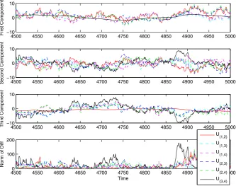
Fig. 2 Deficiency between the full and approximate processes for the 3-state chain. Comparison of the deficiencyU(i,j )(t )=X(i,j )(t )−X(t )projected onto each component of the system of trajectories of
an OU process onR3.Top panel:U(3,4)is essentially zero which shows that reduced processX(3,4)is
optimal for preserving the accuracy of the first component.Second panel: no reduced process is optimal for preserving the accuracy of the second component.Third panel:U(1,2)is essentially zero which shows that
X(1,2)is optimal for preserving the accuracy of the third component (the conducting state in our 3-state
example).Bottom panel: squared norm of the deficiencyU(i,j )2= X(i,j )−X2
˜
X=X(i,j,k) to explicitly define which columns of the full matrix B are neglected
in the approximate process, i.e. which stochastic transitions are neglected. We are interested in the accuracy of the approximation of the trajectory itself.
Figure2 illustrates the deficiency U(i,j )(t )=X(i,j )(t )−X(t ) between the full
process and all possible two noise source reductionsX(i,j ) on the 3-state chain, as
Table 2 Table of discrepancies
MU(i,j,k)=M(X(i,j,k)−X)
for the 3-state Markov process. The discrepancyMU(1,2)
(marked by∗) corresponds to reduced processX(1,2)
projected onto the third component, which is the optimal two-edge-neglecting
approximation ofXfor this example, in agreement with Schmandt and Galán [14]
MU(i,j,k) Rk Value
MU(1) R1 0.0417
MU(2) R2 0.0417
MU(3) R3 0.2917
MU(4) R4 0.2917
MU(1,2) R1+R2 0.0833*
MU(3,4) R3+R4 0.583
MU(1,3) R1+R3 0.3333
MU(1,4) R1+R4 0.3333
MU(2,3) R3+R3 0.3333
MU(2,4) R2+R4 0.3333
MU(1,2,3) R1+R2+R3 0.375
MU(1,2,4) R1+R2+R4 0.375
MU(1,3,4) R1+R3+R4 0.625
MU(2,3,4) R2+R3+R4 0.625
If we fix a point in the underlying sample space (a choice of four Poisson processes
Yk(t )in the systemN (t ) or a choice of four white noise processes dWk(t ) in the
systemX(t )) and then choose to neglect the fluctuations in two of the four, i.e. by replacingYk(t )withE[Yk(t )]ordWk(t )with zero, respectively, then the question is:
which choice leads to the most accurate representation of the process as seen by the measurement?
By Lemma1, we have the following expression for the edge importance termsRk:
Rk=
3
i=2 3
j=2
−1
λi+λj
Mvi
viζk
ζkvj
vjM. (16)
Evaluating this expression for the measurement functionalM= [0,0,1]yields
R1=R2=0.0417, R3=R4=0.2917.
Table2shows the stationary variance of the discrepancyMU(i,j,k)=M(X(i,j,k)−
X) for all possible reduced processes X(i,j,k). For instance, X(1,2) is the reduced
process that neglects fluctuations in reactions 1 and 2 and the stationary variance ofMU(1,2) isR1+R2=0.0833. Note thatX(1,2) is the optimal reduced process
in terms of the Schmandt and Galán stochastic shielding approximation (among all approximations neglecting exactly two edges) for the 3-state chain.
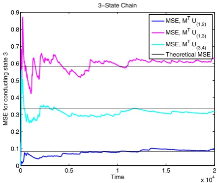
Figure3shows the mean squared error as a function of time forMU(i,j )(t )
cor-responding to the three classes of reduced processesX(i,j )(t )on the 3-state chain
(i.e., the classes areX(1,2),X(3,4), and{X(1,3), X(1,4), X(2,3), X(2,4)}, corresponding
to the three differentMU(i,j )(t )values shown in Table2above). The error
Fig. 3 Mean squared errors for the 3-state chain. Comparison of mean squared errors of
MU(i,j )in the 3-state chain,
i.e. the projection ofU(i,j )onto
the third component. The theoretical MSE values are computed by summing the appropriate edge importance valuesRk.MU(1,2)has the
smallest MSE out of the three classes of 2-noise source reduced process, showing that, as observed by Schmandt and Galán,X(1,2)is optimal at
preserving the accuracy of the full process with respect to the third component of the system
Mζ1=Mζ2=0,Mζ3=1, andMζ4= −1 we confirm the claim made by Schmandt
and Galán [14] that reactions 3 and 4 are important whereas reactions 1 and 2 are unimportant in terms of stochastic shielding for this 3-state example.
3 Analysis of Stochastic Shielding for a Random Graph Ensemble
For any particular Ornstein–Uhlenbeck process on a graph, Lemma1provides the edge importance valuesRk (Eq.10), which may be used to compute explicitly the
contribution to the deficiency made by neglecting any particular reaction, relative to a given measurement vectorM. In order to make general observations about the stochastic shielding approximation, we now consider an ensemble of random graphs. The proof of our main result (Theorem2, restated below) will rely on properties of the joint distribution of components of eigenvectors ofL, the graph Laplacian. Previously, we usediandj to refer to the source and destination nodes in a reaction. In this section, we will adapt the notation so that edgekis a reaction from nodel−to nodel+, denoted byl±(k)∈E(see Eq.17). In this section,iandjwill instead index eigenvectors ofL.
ζk=
⎛ ⎜ ⎜ ⎜ ⎜ ⎜ ⎜ ⎜ ⎜ ⎜ ⎜ ⎜ ⎝
ζk(1)
.. . ζk(l−)
.. . ζk(l+)
.. . ζk(n)
⎞ ⎟ ⎟ ⎟ ⎟ ⎟ ⎟ ⎟ ⎟ ⎟ ⎟ ⎟ ⎠ = ⎛ ⎜ ⎜ ⎜ ⎜ ⎜ ⎜ ⎜ ⎜ ⎜ ⎜ ⎜ ⎝ 0 .. . −1 .. . 1 .. . 0 ⎞ ⎟ ⎟ ⎟ ⎟ ⎟ ⎟ ⎟ ⎟ ⎟ ⎟ ⎟ ⎠ . (17)
are available, we use “O” notation. For the reader’s convenience, we restate Theo-rem2.
Theorem 2 Given an ensemble of symmetric directed graphs G=(V,E) with n nodes satisfying assumptionsA0–A5 (see Sect.3.1),a binary measurement vector M∈ {0,1}nsatisfying0<iMi∼O(1)asn→ ∞,and a stoichiometry vectorζk
corresponding to thekth reaction,the mean squared errorRkresulting from
neglect-ing thekth reaction has expected value
E[Rk|M] =
σk2|Mζk|
nC +O
n−q, asn→ ∞, for someq >1, (18)
where the constantCdepends on the mean edge weight.
In other words, since
Mζk=
1, if reactionkconnects nodes with differentMvalues,
0, if reactionkconnects nodes with the sameMvalue (19)
reactions connecting nodes with identical values ofM have a small contribution to the error, so these reactions can be neglected under the stochastic shielding approxi-mation. This result relies on a list of assumptions which are described in detail below. The proof of this theorem requires Lemma3, which is stated after the assumptions and proved in AppendixC.3.
3.1 Assumptions on the Random Graph Ensemble
We state a sequence of assumptions on the random graph ensemble needed to estab-lish our main result. Each assumption is reasonable for a broad class of graphs of interest, for reasons articulated in the Remarks following each assumption. In several instances we impose on our random graph ensemble, as assumptions, properties that are known to hold for broad classes of random matrices, such as the Wigner ensemble [19,20]. The ensemble we consider is not equivalent to a generalized Wigner ensem-ble. Nevertheless, for the reasons detailed below, it appears reasonable, that certain aspects of the eigenvector and eigenvalue distribution may be similar in the two cases. We consider an ensemble of symmetric directed graphsG=(V,E)with|V| =n. Letζk be the stoichiometry vector corresponding to thekth reaction (Eq.17) and
let(λi, vi)denote the eigenpairs of the graph LaplacianL=(A−D) listed with
eigenvalues in descending order. We assume that the eigenvector components arel2
-normalized with mean 0 and variance 1/n, and we assume the following:
A0. (Following [21].) Let aij ≥0, the entries of the adjacency matrix, be random
variables defined on a common probability space, with{aij,1≤i < j≤n}
in-dependent (but not necessarily identically distributed), withaij=aj i,E[aij] =
μA, V[aij] =σA2>0 for all 1≤i < j ≤n, and sup1≤i<j≤nE|(aij−μA)/
A1a. The graph is drawn from a random ensemble with the property that the eigen-valuesλi and eigenvectorsvi of the associated graph Laplacian are nearly
in-dependent. That is, for anyi, j, k, l∈ {1, . . . , n}and arbitrary measurable func-tionsf :R2→Randg:Rn×Rn→R
Ef (λi, λj)g(vk, vl)
=Ef (λi, λj)
Eg(vk, vl)
+O 1 n4
, asn→ ∞. (20)
Remark 1a: Assumption A1 holds for the symmetric Gaussian ensemble as well as for the more general Wigner ensemble [19,20]. Indeed for these ensembles the eigenvalues and eigenvectors are independent. The weaker assumption, that they are at most weakly correlated, appears reasonable for e.g. the ensemble of graph Laplacians obtained from the symmetric Erdös–Rényi random graph ensemble.
A1b. The graph is drawn from a random ensemble with the property that the joint (eigenvalue, eigenvector) distribution is nearly invariant under permutation of eigenvectors. That is, for anyi, j, k, l∈ {1, . . . , n}
Ef (λi, λj)g(vi, vj)
=Ef (λi, λj)g(vk, vl)
+O 1 n4
, asn→ ∞. (21)
Remark 1b: The symmetric Gaussian and Wigner ensembles are fully invariant under permutation of eigenvectors, and the weaker assumption of near invari-ance appears reasonable for the Erdös–Rényi ensemble. In particular, the pair
(λ−1
i+λj),(M
v
iviζkζkvjvjM)appearing in the definition ofRk (Lemma1)
are assumed to be approximately uncorrelated. This assumption is reasonable by virtue of the approximate rotational symmetry of the eigenvector distribu-tion under our choice of random graph model, which we expect to be close (heuristically) to the eigenvector distribution of the symmetric Gaussian en-semble [19,20].
A2. E[vi(l)] =0 for anyi, l∈ {1, . . . , n}wherevi(l)denotes thelth component of
theith eigenvector.
Remark 2a: Note thatE[vi(l)2] =1/n by thel2-normalization of the
eigen-vectors becausev2=ln=1v(l)2=1 for each eigenvectorv. This
normal-ization leaves a 2-fold ambiguity in the choice of eigenvectorv. Since+vand −v both have v2=1, we choose randomly between them so that the first
non-zero component is positive with probability 1/2.3
Remark 2b: By the symmetry of our random graph ensemble under the symmet-ric group acting on the change of labels, assumption A2 holds not just for the Gaussian and Wigner ensembles, but for any reasonable symmetric ensemble. In particular, it holds for the symmetric Erdös–Rényi random graph ensemble.
3In contrast, Tao and Vu [20] always choose the first non-zero component to be positive to remove this
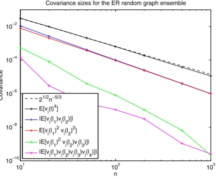
Fig. 4 Covariance sizes for the Erdös–Rényi random graph ensemble. Pairwise and fourth order covari-ance sizes of the eigenvector components of the graph Laplacian for the Erdös–Rényi random graph en-semble. To evaluate the fourth moment and the mixed moments listed inthe legend, we computed the average value over≥100 independent samples for each value ofn. Empirically, the expected value of
vi(l)4is approximately
√
2n−5/3(black);the dashed lineis√2n−5/3. The absolute value of the expec-tation ofvi(l1)vj(l2)isn−2ifi=j(blue) and essentially 0 ifi=j(data not shown; the average value
was 10−19or smaller). The expectation ofvi(l1)2vi(l2)2is approximatelyn−2(red). The absolute value
of the expectation ofvi(l1)2vi(l2)vi(l3)andvi(l1)vi(l2)vi(l3)vi(l4)are both of ordern−3(greenand
magenta). This is numerical evidence for assumptions A3–A5 below
A3. For anyi, j∈ {2, . . . , n}andl, l∈ {1, . . . , n}, a. E[vi(l)vj(l)] =O(n−3)asn→ ∞, fori=j.
b. E[vi(l)vi(l)] =O(n−2)asn→ ∞, forl=l.
Remark 3: Figure4provides numerical evidence for the plausibility of assump-tion A3 in the Erdös–Rényi case. As described in the figure, the empirical ex-pectation ofvi(l)vi(l)scales asO(n−2)for 10≤n≤1000; over this range the
empirical expectation ofvi(l)vj(l),i=j, is within machine error (≤10−19)
of zero.
A4. For anyi∈ {2, . . . , n}andl, l∈ {1, . . . , n},
a. E[vi(l)4] =O(n−q)asn→ ∞, for someq >1.
b. E[vi(l)2vi(l)2] =O(n−2)asn→ ∞, forl=l.
Remark 4: Assumption A4a holds for the Gaussian case for q=2. For the Erdös–Rényi case, empirically we see that assumption A4a holds forq≈5/3 as shown in Fig.4. Specifically, empirical evidence suggests thatE[vi(l)4] ≈
√
2n−5/3in this case.
A5. Suppose thatp1,p2,p3, andp4are nonnegative integers with4m=1pm=4,
at least three of which are non-zero. Then for any i∈ {2, . . . , n}and for any distinct components{l1, l2, l3, l4}
Evi(l1)
p1v
i(l2)
p2v
i(l3)
p3v
i(l4)
p4=On−3
asn→ ∞. (22)
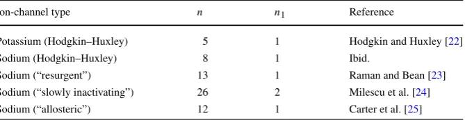
Table 3 Total number of states (n) and number of conducting states (n1) for different ion-channel models.
Empirically based model refinements have led to increasing numbers of channel states, without dramati-cally increasing the number of conducting states
Ion-channel type n n1 Reference
Potassium (Hodgkin–Huxley) 5 1 Hodgkin and Huxley [22]
Sodium (Hodgkin–Huxley) 8 1 Ibid.
Sodium (“resurgent”) 13 1 Raman and Bean [23]
Sodium (“slowly inactivating”) 26 2 Milescu et al. [24]
Sodium (“allosteric”) 12 1 Carter et al. [25]
components of a Wigner or Gaussian random matrix, different versions have been established by Tao and Vu [20] and Knowles and Yin [19]. Figure4 pro-vides numerical evidence for the plausibility of assumption A5 in the Erdös– Rényi case.
In addition to assumptions A0–A5 on the random graph ensemble, the statement of Theorem2 places an assumption on the measurement vectorM∈ {0,1}n. This vector contains n1>0 ones and n0>0 zeros such that n1+n0=n. We assume
n1=O(1)asn→ ∞, that is, we exclude the case wheren1grows without bound as
ngrows. (IfMhas the same value for all nodes, the output is constant and the error is identically zero. The expression in Theorem2holds trivially so we ignore this case.) To motivate this assumption, Table3shows the total number of states (n) and the number of conducting states (n1) for representative ion-channel models. Model
re-finements driven by empirical evidence have tended to increase the total number of states relative to Hodgkin and Huxley’s original model, without significantly increas-ing the number of conductincreas-ing states.
Although assuming thatn1=O(1) is biologically plausible, we make this as-sumption mainly for technical reasons as indicated in the proof of Theorem2. We note, however, that in the numerical example in Sect.3.3, the conclusions of Theo-rem2appear to hold equally well whenn1=n2=n/2.
Lemma 3 If assumptionsA0–A5hold andM∈ {0,1}nsatisfies0<iMi∼O(1)
asn→ ∞.Then asn→ ∞,
A. E[Mviviζk] =E[
l∈1Mvi(l)(vi(l+)−vi(l−))] =
1
nMζk+O(n−
2).
B. E[Mvivi ζk]2=E[
l∈1Mvi(l)(vi(l+)−vi(l−))]
2= 1
n2|Mζk| +O(n−4).
C. E[(Mviviζk)2] =E[(
l∈1Mvi(l))
2(v
i(l+)−vi(l−))2] =O(n−q) for some
q >1.
3.2 Proof of Main Theorem
Suppose assumptions A0–A5 hold andM∈ {0,1}n satisfies 0<
iMi ∼O(1)as
n→ ∞. By Lemma1,Rk denotes the contribution of thekth reaction to the
defi-ciency of the approximate process. Given the measurement vectorM, we have (ex-actly)
E[Rk|M] =E
σk2
n
i=2
n
j=2
−1
λi+λj
Mvivi ζk
ζkvjvjM
. (23)
This expectation is taken over the space of symmetric directed graphs G=(V,E)
where edgekis chosen at random from the set ofn2possible bidirectional edges. If
l±(k) /∈E, thenE[Rk|M] =0.
If the graph Laplacian were drawn from a symmetric Gaussian ensemble (or Wigner ensemble; see [19,20]), then the eigenvalues and the eigenvectors would be independent. For other ensembles we impose the weaker condition ofnear inde-pendence(assumption A1a), which in this case means that for eachi≥2 andj≥2, we assume
E −1 λi+λj
Mviviζk
ζkvjvjM
=E −1 λi+λj
EMviviζk
ζkvjvjM
+O 1 n4
, asn→ ∞. (24)
Under assumption A1b, the joint distribution of eigenvalues and eigenvectors is approximately separable into the product of two measures, one for the eigenvalues and a second for the eigenvectors. In this case the expectationE[(λ−1
i+λj)]in the sum (23) can be replaced by its average,
S≡ 1 (n−1)2
n
i=2
n
j=2
−1
λi+λj
, (25)
to obtain
E[Rk|M] =σk2E[S]E
n
i=2
n
j=2
Mviviζk
ζkvjvjM
+O 1 n2
. (26)
As shown in [21], assumption A0 implies that the empirical eigenvalue distribution for the graph LaplacianL,
˜
Fn(x)=
1
n
n
i=1 I
λi√+nμA
nσA
≤x
, (27)
converges weakly (with probability one) asn→ ∞to the free convolutionγ of the semicircle law,ρsc(x)=21π√4−x2I (|x| ≤2), with the standard Gaussian,g(x)=
exp[−x2/2]/√2π. The measureγ becomes concentrated aroundλi ≈ −nμA as n
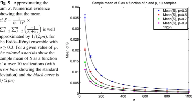
Fig. 5 Approximating the sumS. Numerical evidence showing that the mean ofS= 1
(n−1)2×
n i=2
n j=2
−
1
λi+λj
is well approximated by 1/(2pn), for the Erdös–Rényi ensemble with
p≥0.3. For a given value ofp,
the colored asterisksshow the sample mean ofSas a function ofnover 10 realizations (with
error barsshowing the standard deviation) andthe black curveis 1/(2pn)
asn→ ∞. Therefore, by imposing assumption A0 and settingC=2μA, we have
E[S] →1/(nC), asn→ ∞, yielding in the limit
E[Rk|M] =
σk2 nCE
n
i=2
n
j=2
Mviviζk
ζkvjvjM
+O 1 n2
. (28)
For the Erdös–Rényi ensemble with n nodes and edge probabilityp, we have
E[S] →1/(nC) for C=2p. Figure 5 shows that the sample mean ofS over 10 realizations (i.e. 10 different Erdös–Rényi random graph configurations with the same parameters) rapidly approaches 1/(2pn), asnincreases, for values ofpranging from 0.3 to 0.9. As the factor of 1/nis common across allk, it does not affect the stochastic shielding argument.
To prove Theorem2, we will show that
E
n
i=2
n
j=2
Mviviζk
ζkvjvjM
=
1+O(n1−q), |Mζk| =1,
O(n1−q), |Mζk| =0,
asn→ ∞, (29)
for some q >1, corresponding to the parameter q appearing in assumption A4. This dichotomy is the basis for neglecting the edgesk such that Mζk =0, as in
the stochastic shielding approximation. To do this, we will use assumption A3a and Lemma 3 to show the following:
E
n
i=2
n
j=2
Mviviζk
ζkvjvjM
(30)
=
n
i=2
j=i
EMviviζk
Mvjvjζk
+
n
i=2
EMviviζk
2
=
n
i=2
j=i
EMvivi ζk
EMvjvjζk
+
n
i=2
EMviviζk
2
+O 1 n
, asn→ ∞ (32)
=Mζk+O
n1−q, asn→ ∞. (33) It suffices to show that the first term in Eq.32is
n
i=2
j=i
EMviviζk
EMvjvjζk
=Mζk+O
1
n
, asn→ ∞, (34)
and the second term is
n
i=2
EMviviζk
2
=On1−q, asn→ ∞. (35)
Starting with the first term in Eq. 31, it follows from assumption A3a that, as
n→ ∞,
EMviviζk
Mvjvjζk
=EMvivi ζk
EMvjvjζk
+O 1 n3 (36) which means n
i=2
j=i
EMviviζk
Mvjvjζk
=
n
i=2
j=i
EMviviζk
EMvjvjζk
+O 1
n
. (37)
We can expand the left hand side of Eq. 34 by using the definitions Mvi =
l∈1Mvi(l)andv
i ζk=vi(l+)−vi(l−), which yield n
i=2
j=i
EMviviζk
EMvjvjζk
(38)
=(n−1)(n−2)EMviviζk
EMvjvjζk
(39)
=(n−1)(n−2)E
l∈1M
vi(l)
vi(l+)−vi(l−)
2
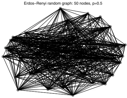
Fig. 6 Erdös–Rényi random graph. Realization of an Erdös–Rényi random graph with
n=50 nodes and edge probabilityp=0.5
By Lemma3part B, we have thatE[l∈1
Mvi(l)(vi(l+)−vi(l−))]
2= 1
n2|Mζk| +
O(n−4), asn→ ∞. Continuing Eq.40above we have =(n−1)(n−2)
1
n2Mζk+O
n−4 (41) =Mζk+O
n−1 (42) asn→ ∞, which establishes the first term (Eq.34).
We now focus on the second term in Eq.32. In Lemma3part C, we establish that asn→ ∞
EMviviζk
2
=E
l∈1M
vi(l)
2
vi(l+)−vi(l−)
2
=On−q. (43)
Hence,(n−1)E[(l∈1
Mvi(l))
2(v
i(l+)−vi(l−))2] =O(n1−q)as n→ ∞, which
establishes the second term (Eq.35). Therefore, we have established Theorem2.
3.3 Symmetric Erdös–Rényi Random Graph Ensemble
Many varieties of random graphs have been used to describe biological systems [26,
27]. Here, we restrict attention to an ensemble of symmetric Erdös–Rényi random graphsG(n, p)onnnodes, for which each of(n2−n)/2 possible bidirectional edges occurs independently with probabilityp [28,29]. Consider a graph drawn from the Erdös–Rényi ensemble forn=50 andp=0.5. See Fig.6for an example. TakeAto be the unweighted adjacency matrix (αk∈ {0,1}) and letσk=1 for all reactionskso
that thekth column of the matrixBis exactly the stoichiometry vector for reactionk. Specifying any measurement vectorM∈ {0,1}50 induces a partition of edges into “important” (type 0–1) or “unimportant” (types 0–0 or 1–1) classes. LetEI be the set
of important edges andEU be the set of unimportant edges. Clearly,E=EI∪EU. In
Fig. 7 Rank order of edge importance for the Erdös–Rényi ensemble. Edge importance valuesRkplotted in descending
order for the process on an Erdös–Rényi random graph with 50 nodes, edge probability 0.5, and measurement functionalM
such that half the nodes are labeled 1 and the other half are 0. There is a clear separation between the important edges (type 0–1) and unimportant edges (types 0–0 and 1–1). The cluster of important edges has a meanRkvalue of 1/50=0.02
whereas the unimportant cluster lies belowthe lineat
√
2n−5/3≈0.0021
Theorem2says that if the matrix of eigenvector components of the Erdös–Rényi graph Laplacian is sufficiently similar to a random matrix drawn from the Gaussian ensemble (in terms of assumptions A0–A5) then one would expect the partitioning of theRkinto two clusters. One cluster, containing the important edges, will be centered
at 1/n. A second cluster, containing the unimportant edges, will have smaller Rk
values (O(n−q)whereq >1 is governed by the fourth moment; see assumption A4a in Sect.3.1). To the extent to which this similarity to the Gaussian ensemble holds, our calculation ofRk involves projecting the measurement vectorMand the vectors
ζk onto randomly chosen subspaces ofRn.
As shown in Fig.4, assumptions A0–A5 appear to be satisfied for the symmetric Erdös–Rényi random graph ensemble. In particular, the fourth moment of the eigen-vector components (assumption A4a) appears to hold empirically for q≈5/3; in particular, we find that, empirically,E[vi(l)4] ≈
√
2n−5/3. This behavior suggests that the unimportant edges should have a meanRkvalue
√
2n−5/3. Settingn=50, for example, we would expect one cluster ofRk values centered at 1/50=0.02 for
k∈EI and another cluster close to
√
2·50−5/3≈0.0021 fork∈EU. Figure7shows
the rank order of edge importance valuesRk corresponding to them reactions in
the Erdös–Rényi random graph. The top cluster is centered at 0.02 (upper horizon-tal red line) and the bottom cluster is bounded above by 0.0021 (lower horizontal red line) consistent with Theorem2for the Erdös–Rényi random graph ensemble with 50 nodes and edge probabilityp=0.5. Since the measurement functionalMis binary, we see a significant gap between the two clusters, as expected. If the components of
Mare graded, i.e. drawn uniformly from the unit interval, then this curve appears to be smooth (see discussion in Sect.5).
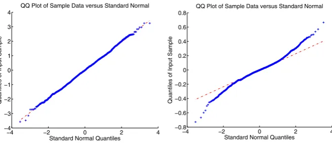
Fig. 8 Comparison of eigenvector components of the graph Laplacian in the Erdös–Rényi and Gaussian ensembles. Numerical evidence illustrating that the eigenvector components of the graph Laplacian for the symmetric Erdös–Rényi random graph ensemble are close to Gaussian distributed (to one standard deviation).Left: quantile–quantile plot for a Gaussian random matrix with N(0,1/50) entries.Right: quantile–quantile plot of eigenvector components for the Erdös–Rényi case withn=50 nodes and edge probabilityp=0.5
Nevertheless, Theorem2predicts that there will be two clusters ofRk values as
de-scribed above and shown in Fig.7for the Erdös–Rényi case withn=50 andp=0.5.
4 Application: Stochastic Shielding of Hodgkin–Huxley Channels Under Voltage Clamp
Hodgkin and Huxley’s (HH) model for the generation and propagation of action potentials along the giant axon of the squidLoligolies at the foundations of mod-ern neuroscience [22,30]. In the classic HH model, action potentials are generated through the interaction of a leak current and two voltage-gated ionic currents, carried by a sodium ion specific channel and a potassium ion specific channel. The potas-sium channel comprises four identical subunits that open and close independently with voltage-dependent rates. The channel carries a current when all four subunits are in the open state. At the molecular level, a single channel can be represented as a continuous time Markov jump process on a chain of five states, the fifth of which has non-zero conductance. Of the eight transitions connecting states along this chain, only the last two connect states with different conductances, therefore the stochastic shielding approximation would preserve the fluctuations of these transitions and not the other six.
The sodium channel involves two types of subunits, an activation subunit (“m”) present in three identical copies, and an inactivation subunit (“h”) present in a single copy.4The resulting graph has eight distinct states connected by 20 different transi-tions, each occurring with a voltage-dependent rate [31–33]. Four of these 20
tran-4Modern measurements of purified sodium channel preparations suggest the presence of four activation
sitions connect states with differing conductance values (zero versus non-zero); the fluctuations of the remaining 16 transitions are ignored under the stochastic shielding approximation.
Schmandt and Galán compared simulations of a system comprising 5000 individ-ual potassium channels and 25000 individindivid-ual sodium channels, both with and without the stochastic shielding approximation. It is possible to construct an exact simulation scheme, analogous to Gillespie’s stochastic simulation algorithm [34], that takes into account the nonstationarity of the transition rates (propensities) arising from their voltage dependence [35]. However, Schmandt and Galán used a discrete time ap-proximation to this process. AppendixAdiscusses Schmandt and Galán’s approach in more detail. Here we apply our analysis to evaluate the edge importanceRk of
each transition in the graph for the classic HH potassium and sodium channels, re-spectively. Rather than consider the case of time-varying transition rates, we restrict attention to the “voltage clamped” case. If the membrane potential is experimentally held constant for a given cell, the per capita transition rates remain constant and the fluctuating ion-channel population forms a stationary Markov process. In particular, our analysis approximates this stationary population process with a linear multidi-mensional Ornstein–Uhlenbeck process (see AppendixB); this approximation is rea-sonable given the large numbers of individual channels considered in Schmandt and Galán’s simulations.
In general, the ion-channel state graphs for the potassium and sodium channels in the HH model have graph LaplaciansLthat are not symmetric. Therefore, we need to modify our definition of the edge importanceRk(Eq.10) in order to apply our results.
WhenLis not symmetric, we will assume thatLis nevertheless diagonalizable, i.e. that there are eigenvaluesλi and a biorthogonal system of vectorsvi,wi (right and
left eigenvectors) satisfying
Lvi=λivi,
wi L=λiwi, (44)
wivj=δij.
In this case the decomposition ofLbecomesL=iλiviwi , and the definition of
Rk is modified as follows:
Rk=σk2 n
i=2
n
j=2
−1
λi+λj
Mvi
wiζk
ζkwj
vjM. (45)
4.1 Hodgkin–Huxley Potassium Channel
The potassium channel state graph in the Hodgkin–Huxley model is a 5-state chain with one conducting state. Following the tau-leaping construction (AppendixB) we consider a stationary OU process X(t )∈R5, with linear measurement functional
Fig. 9 Illustration of the Hodgkin–Huxley potassium channel state graph. This is a 5-state chain where state 5 is the conducting state. The eight reactions are labeled inblueand are used to define the edge importance valuesRkin the figures below. The reaction ratesαnandβnare voltage-dependent as defined
by Eqs.47–48
(weighted) adjacency matrixAis
A=
⎛ ⎜ ⎜ ⎜ ⎜ ⎝
0 4αn(V ) 0 0 0
βn(V ) 0 3αn(V ) 0 0
0 2βn(V ) 0 2αn(V ) 0
0 0 3βn(V ) 0 αn(V )
0 0 0 4βn(V ) 0
⎞ ⎟ ⎟ ⎟ ⎟
⎠, (46)
which is evidently not symmetric. The voltage-dependent transition rates are given by
αn(V )=
0.01(V+55)
1−e(−0.1(V+55)), (47)
βn(V )=0.125e−(V+65)/80. (48)
Then the graph LaplacianL=(A−D)is voltage-dependent and is given by
L=
⎛ ⎜ ⎜ ⎝
−4αn(V ) βn(V ) 0 0 0
4αn(V ) −(βn(V )+3αn(V )) 2βn(V ) 0 0
0 3αn(V ) −2(βn(V )+αn(V )) 3βn(V ) 0
0 0 2αn(V ) −(3βn(V )+αn(V )) 4βn(V )
0 0 0 αn(V ) −4βn(V )
⎞ ⎟ ⎟ ⎠,
since the entries in the diagonal matrixDare the weighted out-degrees of each node for a given voltageV, i.e. Dii(V )=
5
j=1Aij(V ). The matrixB is also
voltage-dependent. Recall that thekth column ofBcorresponds to thekth reaction, and this can be written asσk(V )ζk. Ifrk is the per capita rate of reactionk (transition from
nodei(k)toj (k)), thenσk(V )=
rk(V )N¯i(V )whereN¯i(V )is the average number
of channels at stateiat equilibrium for voltageV. Hence,Bis given by
B=r1(V )N¯i(1)(V )ζ1, . . . ,
rk(V )N¯i(k)(V )ζk, . . . ,
rm(V )N¯i(m)(V )ζm
. (49)
Figure10shows the edge importanceRkas a function of voltage for each reaction
k∈ {1, . . . ,8}in the potassium channel state graph. Note that since the process is at steady state, and respects detailed balance, the mean flux due to the two reactions connecting the same pair of nodes will be equal and opposite. Thus, in this case,
Fig. 10 Hodgkin–Huxley potassium channel: edge importance. This figure shows edge importanceRkas a
function of voltage in the range [−100,100]mV for each reactionk∈ {1, . . . ,8}.The blue curvecorresponds to edges 7 and 8 (R7=R8), the transitions
between state 4 and conducting state 5, which is the largestRk
value in the voltage range above. If neglected, these two reactions would have the highest contribution to the error
to edges 7 and 8, the transitions between state 4 and conducting state 5, and has the largest edge importance value in the voltage range[−100,100]mV. This says that if either or both of these reactions are neglected, they would have the highest contribution to the error.
Physically, it is the current rather than the state occupancy that holds the greatest interest. The current through a population of potassium channels with net conduc-tancegis I=g(V −Vk); hereVk= −77 mV is the potassium reversal potential,
and the conductanceg=goNo is the product of the unitary or single channel
con-ductancegowith the total number of channels in the open state,No. The variance of
the current is therefore(go(V −Vk))2times the variance of the occupancy number,
meaning that near the reversal potential, the current can have low variance even if the channel state has high variance. For convenience we setgo=1, which amounts to a change of nominal units for measuring the conductance.
Figure11shows the variance of the nominal current,Rk∗(V−Vk)2as a function
of voltageV for each reactionkfor the potassium channel. In addition to having the highest edge importance curve, the blue curveR7=R8also has the highest variance
(left panel). The right panel shows the probability of being in each state as a function of voltage.
4.2 Hodgkin–Huxley Sodium Channel
The sodium channel state graph in the Hodgkin–Huxley model consists of two linked 4-state chains, for a total of eight states, including one conducting state, and 20 reactions. Again following the tau-leaping construction (AppendixB) we consider a stationary OU process X(t )∈R8, with linear measurement functional
Fig. 11 Hodgkin–Huxley potassium channel: variance of current and state occupancy.Left: variance of the currentRk∗(V−Vk)2as a function of voltageV for each reactionkwhereVk= −77 mV is the
reversal potential for the potassium channel.The blue curveR7=R8 has the highest variance.Right:
leading eigenvector components (normalized so that the components sum to 1) as a function of voltage
Fig. 12 Illustration of the Hodgkin–Huxley sodium channel. This channel has eight states, where state 8 is the conducting state, and 20 reactions. The reactions are labeled inblueand are used to define the edge importance valuesRkin the figures below. The reaction ratesαm,αh,βm, andβhare voltage-dependent,
defined in Eqs.51–52
The adjacency matrix in this case is
A=
⎛ ⎜ ⎜ ⎜ ⎜ ⎜ ⎜ ⎜ ⎜ ⎜ ⎝
0 3αm(V ) 0 0 αh(V ) 0 0 0
βm(V ) 0 2αm(V ) 0 0 αh(V ) 0 0
0 2βm(V ) 0 αm(V ) 0 0 αh(V ) 0
0 0 3βm(V ) 0 0 0 0 αh(V )
βh(V ) 0 0 0 0 3αm(V ) 0 0
0 βh(V ) 0 0 βm(V ) 0 2αm(V ) 0
0 0 βh(V ) 0 0 2βm(V ) 0 αm(V )
0 0 0 βh(V ) 0 0 3βm(V ) 0
⎞ ⎟ ⎟ ⎟ ⎟ ⎟ ⎟ ⎟ ⎟ ⎟ ⎠
,
(50)
where the voltage-dependent entries are defined by
αm(V )=
0.1(V+40)
1−e−(V+40)/10, βm(V )=4e−
Fig. 13 Hodgkin–Huxley sodium channel: edge importance. This figure shows edge importanceRkas a
function of voltage in the range [−100,100]mV for each reactionk∈ {1, . . . ,20}.The magenta curvecorresponds to edges 11 and 12 andthe yellow curvecorresponds to edges 19 and 20 (transitions between the conducting state 8 and its two nearest neighbors, states 7 and 4, respectively). Note that
R11=R12(magenta) has the
highest edge importance in the voltage range[−100,−25]mV andR19=R20(yellow) has the
highest value in the range [−25,100]mV
αh(V )=0.07e−(V+65)/20, βh(V )=
1
1+e−(V+35)/10. (52)
The graph LaplacianL=(A−D)is
L=
⎛ ⎜ ⎜ ⎜ ⎜ ⎜ ⎜ ⎜ ⎜ ⎜ ⎜ ⎝
−D11(V ) βm(V ) 0 0
3αm(V ) −D22(V ) 2βm(V ) 0
0 2αm(V ) −D33(V ) 3βm(V )
0 0 αm(V ) −D44(V )
αh(V ) 0 0 0
0 αh(V ) 0 0
0 0 αh(V ) 0
0 0 0 αh(V )
βh(V ) 0 0 0
0 βh(V ) 0 0
0 0 βh(V ) 0
0 0 0 βh(V )
−D55(V ) βm(V ) 0 0
3αm(V ) −D66(V ) 2βm(V ) 0
0 2αm(V ) −D77(V ) 3βm(V )
0 0 αm(V ) −D88(V )
⎞ ⎟ ⎟ ⎟ ⎟ ⎟ ⎟ ⎟ ⎟ ⎟ ⎟ ⎠
,
whereDii(V )=
8
j=1Aij(V )from the adjacency matrix above (Eq.50). The matrix
Bis also voltage-dependent and is given by the general expression in Eq.49. Figure13shows the edge importanceRkas a function of voltage for each reaction
k∈ {1, . . . ,20}for the sodium channel state graph. The sodium channel also satisfies detailed balance, so each pair of complementary reactions ki,ki+1 connecting the

![Table 2 Table of discrepanciesexample, in agreement withSchmandt and Galán [M⊺U(i,j,k) = M⊺(X(i,j,k) −X)for the 3-state Markov process.The discrepancy M⊺U(1,2)(marked by ∗) corresponds toreduced process X(1,2)projected onto the thirdcomponent, which is the optimaltwo-edge-neglectingapproximation of X for this14]](https://thumb-us.123doks.com/thumbv2/123dok_us/915755.1589441/11.439.159.388.58.251/discrepanciesexample-agreement-withschmandt-discrepancy-corresponds-thirdcomponent-optimaltwo-neglectingapproximation.webp)