ReseaRch aRticle
S
enSitivityA
nAlySiS of Af
ireS
preAdM
odel in AC
hApArrAll
AndSCApeR.E. Clark1*, A.S. Hope1, S. Tarantola2, D. Gatelli2, P.E. Dennison3, and M.A. Moritz4
1Department of Geography, San Diego State University, San Diego, California 92182-4493, USA
2Joint Research Centre of the European Commission, Institute for the Protection and Security of the Citizen,
TP 361, I-21020 Ispra (Va), Italy
3Center for Natural and Technological Hazards, Department of Geography, University of Utah,
Salt Lake City, Utah 84112, USA
4Center for Fire Research and Outreach,
Department of Environmental Science, Policy, and Management, University of California, Berkeley, California 94720, USA
*Corresponding author: Tel.: 001-619-890-5638; e-mail: [email protected]
AbStrACt
Due to a unique combination of environmental conditions, the chaparral shrublands of
southern California are prone to large, intense wildland fires. There is ongoing work in the fire research community to establish whether fuel accumulation or weather conditions are the determining factor in the prevalence of large chaparral fires. This study introduces
a framework for contributing a modeling perspective to understanding these alternative
hypotheses. As models formalize our understanding of the physical process of fire spread,
the sensitivity of the models to the meteorological and fuel inputs should be indicators of their relative importance. A global sensitivity analysis (GSA) was conducted on HFire, a
spatially explicit raster model developed for modeling fire spread in chaparral fuels, based
on the Rothermel spread equations. The GSA provided a quantitative measure of the
importance of each of the model inputs on the predicted fire size. The results indicate that, under extreme weather conditions, wind speed was over three times more influential on predicted fire sizes than any other single model input. This finding supports the idea that fires burning under Santa Ana conditions are primarily driven by high wind speeds.
Future research will involve extending the GSA methodology to quantify the relative
importance of these inputs in terms of the long-term fire regime in chaparral ecosystems.
Keywords: chaparral, global sensitivity analysis, HFire model, Rothermel equations
Citation: Clark, R.E., A.S. Hope, S. Tarantola, D. Gatelli, P.E. Dennison, and M.A. Moritz. 2008.
introduCtion
Southern California is considered among
the most fire-hazardous landscapes in North
America due to a unique combination of environmental conditions that are favorable to
the development of large fires. These
conditions include volatile fuels, dense fuel growth, steep terrain, and recurrent droughts.
The influence of the Santa Ana foehn winds further increases the risk of large fires. In a
Santa Ana event, the normal onshore marine
airflow is replaced by offshore, downslope
winds. The combination of high wind speeds, dry continental air, clear skies, and increased temperatures can rapidly dry fuels. The prevailing conditions during a Santa Ana event, including low relative humidity, high wind speed, and warming, can result in “explosive” burning conditions (Schroeder et al. 1964).
The chaparral shrublands of southern California are dominated by periodic, large,
high-intensity fires (Keeley and Fotheringham 1994, Moritz 1997). The fire research
community has not reached a consensus as to
the impact that fire suppression policies have had on the modern chaparral fire regime (the
size, intensity, and frequency of chaparral
fires). Studies have compared the historic fire
regimes of southern California and Baja California (Minnich 1983, Minnich and Bahre 1995, Minnich and Chou 1997, Minnich 2001)
and have concluded that fire suppression
efforts in southern California result in larger and more contiguous stands of older fuels, and that this fuel accumulation leads to larger and
more intense fire events. These studies
hypothesize that the chaparral landscape, in
the absence of fire suppression policies, would
be a mosaic of stands of younger and older vegetation. Patches of younger vegetation would then serve as natural breaks, preventing
smaller fires from developing into larger fires,
even during Santa Ana events. Younger stands can also can also result in reduced rates of
spread when reburned (Philpot 1977). Tests of the age-dependent hypothesis have analyzed similar historical data but have concluded that there is not a direct relationship between large
fires and fuel accumulation, and that large fires are a natural feature of the chaparral fire regime (Keeley et al. 1999, Keeley and Fotheringham 2001a, Keeley and Fotheringham
2001b, Moritz 2003, Moritz et al. 2004). In all of these studies, one point of agreement has been that Santa Ana winds can be the driving
force behind large fire events.
Fire behavior models are a conceptual representation of the physical process
controlling fire spread. In fire-prone ecosystems, fire behavior models are used for
a number of applications that involve assessing
the various risks associated with wildland fire,
including training support personnel, planning prescribed burns, predicting the behavior of
active fires, and comparing the effects of
various suppression strategies (Andrews 1989). Fire modeling is also important for understanding how this natural ecological process operates on the landscape (e.g., Hargrove et al. 2000). Fire behavior models
can provide significant insight for research on ecological processes where conducting field
studies can be destructive, and where there is a limited amount of data available from historical events.
The purpose of this study was to introduce a framework for incorporating information
from fire behavior model predictions into fire ecology and fire regime research. As models
formalize our understanding of the physical
process of fire spread, the sensitivity of the
models to the meteorological and fuel inputs should be indicators of their relative importance. Sensitivity analysis (SA) is the study of how the variation in the output of the model can be attributed (qualitatively or quantitatively) to the variation in the model inputs (Saltelli 2000). SA is recommended for
quantifying the influence each input,
model, and for assessing uncertainty in the output that is associated with uncertainty in the inputs (Cruz et al. 2003).
This study was also a conceptual validation of HFire, a spatially explicit model developed
for predicting fire spread in chaparral fuels.
The objective was to use SA techniques to quantitatively establish the way in which the output of HFire is dependent on the inputs of fuel and weather conditions. This analysis was
framed in terms of predicting the size of fires
during potential Santa Ana events, and the research hypothesis being tested was that wind speed accounts for more variability in
simulated fire size than fuel-related variables such as fine dead fuel moisture and fuel model.
The modeling framework introduced in this study could be extended by repeating the analysis under a wider range of conditions representative of the climatology of southern California, which would allow for a more complete characterization of the role that weather and fuels play in terms of the modern
chaparral fire regime.
There are few examples of sensitivity
analysis studies in fire research literature,
nearly all of which involve what is referred to as a “local approach” (e.g., Bevins and Martin 1978, Trevitt 1991, Bessie and Johnson 1995, Hargrove et al. 2000, Miller and Yool 2002, Cruz et al. 2003). Local approaches estimate the effect of the variation of a single input or
parameter by keeping all the others fixed at
their nominal values. Local methods are well established and are familiar to most modelers (Campolongo et al. 2000). Local SA serves as an ad-hoc stability analysis, providing a measure of how stable the model is around the best estimates for the inputs (Turanyi and Rabitz 2000). The local approach is not recommended for investigating the sensitivity of non-linear models in which the uncertainty in the output associated with the uncertainty in each input may be of different orders of magnitude (Cukier et al. 1973).
An alternative approach to evaluating model sensitivity is global sensitivity analysis (GSA), where the input factors, which can be model inputs, sub-models, and model
parameters, are defined by their probability
density functions, and all the factors in the analysis vary simultaneously (Saltelli 2000). Representing factors as probability density functions allows for the exploration of the full range of potential values for each input. Samples from these distributions are used as inputs for model simulations, producing a distribution of model output. By decomposing the variance of the model output, the contribution of each input can be assessed. The sensitivity estimate for each factor, known as an “importance” measure, can be written, in, in terms of conditional variance, as:
Si = V[E(Y|Xi )]/V(Y)
where Y is the output variable, Xi is an input factor, V(Y) is the unconditional variance, E(Y|Xi = x*
i) is the expectation of Y conditional on Xi having a given value x*
i. Importance measures can be compared across factors, and
the more influential factors will have higher
scores.
A review of GSA procedures can be found in Saltelli et al. (2004). Salvador et al. (2001) present an application of GSA techniques in
fire modeling research. GSA has been applied to a number of diverse fields, including
environmental policy, population dynamics, chemical reaction, and economic modeling, and a review of these applications is given in Saltelli et al. (2000). The implementation of global methods in other environmental modeling applications suggests that they can
provide useful insight for fire modeling and fire ecology research.
HFire is a spatially explicit fire spread model that was developed for modeling fires
contact-based approach to fire spread (Kourtz
and O’Regan 1971). This approach is very
computationally efficient, allowing
non-uniform time steps based on the amount of
time required for fire to spread from cell to
cell. Similar to FARSITE (Finney 1998), the
semi-empirical Rothermel fire spread equation (Rothermel 1972, with modifications by Albini
1976) is used in HFire to determine the direction and the magnitude of the maximum
rate of fire spread. The Anderson (1983)
empirical relationship, relating wind speed to
the length-to-width ratio of fire spread, is used to calculate fire spread rates in two dimensions. In HFire, a fire spreading through a lattice of
cells has eight degrees of freedom. In any
three-by-three neighborhood of cells, a fire
located at the center of the neighborhood has the potential of spreading to all eight adjacent neighbors. HFire keeps track of the fractional spread distance from cell center to cell center,
allowing the modeled fire to simultaneously
spread to all of its neighboring cells during a time step.
HFire has been demonstrated to be, on average, 92 times faster than FARSITE for
modeling the same fire (Morais 2001). The
faster run times allow for its use for research applications in which large numbers of simulations are required. The model can be
used to simulate single fire events or multiple
events occurring over a period of hundreds of years. Morais (2001) found that HFire was as accurate as FARSITE for modeling two
historical chaparral fires under both extreme
and moderate wind conditions. To date, the
sensitivity of Rothermel-based fire spread
models over full ranges of input variables has not been examined. A GSA of the HFire model is critical for understanding how input
variables used for simulating wildfires contribute to the modeled fire size, and over longer time periods, fire frequency.
MethodS
Sensitivity analysis was implemented by 1) identifying a study area suited to testing the experimental hypotheses; 2) collecting the spatial information needed to run the model; 3)
collecting the temporal input data; 4) defining
a distribution for each input factor based on statistical analysis of the data; 5) sampling from the distributions of the input factors, and executing the model using these samples; 6) performing the sensitivity analysis in order to quantify the relative importance each input factor has on the output of the model; and 7) evaluating the hypotheses based on the results of the sensitivity analysis.
Study Domain
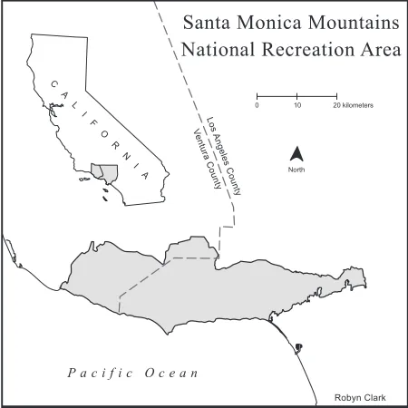
The domain for this study was the Santa Monica Mountains National Recreation Area (SMM), located in Los Angeles and Ventura Counties in southern California (Figure 1). SMM was the original study site for the development of the HFire model. The recreation area is located within southern
���������������������� ������������������������
� � � � � � � � � � � � �
���� �������������� ��������������
� �
� �
� �
� �
� �
� �� �������������
�����������
�����
California’s Mediterranean-type ecosystem. The native vegetation is a mosaic of chaparral, coastal sage scrub, oak woodland, riparian woodland, and grasslands (Radtke et al. 1982).
Over 40 % of the fires in this region are large fires exceeding 400 ha in size, and most of these large fires occur during Santa Ana events
in the fall (Radtke et al. 1982). A nine by nine kilometer subset was selected in an area in the western region of the park that is undeveloped and is predominately chaparral. This study required an area large enough that simulated
fires would not reach the edge of the landscape.
Using a larger subset was not viable due to the layout of the terrain and vegetation and the proximity to urban areas. The terrain and fuels
input data were then used to artificially expand
the subset by creating and inverting mirror images of the study area (Figure 2). This
method alters the orientation of the fuels and the topography, but retains the connectivity between the slope of the terrain and the fuel characteristics.
Input Data
HFire requires a number of temporally and spatially dynamic inputs. The required temporal inputs to HFire are wind speed, wind
direction, fine dead fuel moisture, live
herbaceous fuel moisture, and live woody fuel moisture. The spatial inputs to HFire are slope, aspect, elevation, and fuel characteristics, as well as the coordinates of the ignition location.
Live herbaceous fuel moisture and live woody fuel moisture data were not available for this study domain and period.
Consequently, the decision was made to fix
�������
������������
������������������������
����������������
����������������������� ����������������
��������������� ���������������� ������������
��������������������� �������������
��������������������� �������������
�����
�����
live herbaceous fuel moisture at 50%, and live woody fuel moisture at 70 %. These values were used in the HFire development to represent the lowest live fuel moisture values in the dry season for chaparral fuels (Morais
2001). As fixed values, live herbaceous and
live woody fuel moistures could not be included in the GSA, as variance based approaches involve assessing the importance of each input by decomposing the variance of the output data on the variance of the input data.
Hourly data for wind speed, wind direction,
and fine dead fuel moisture were obtained from
the Western Regional Climate Center (WRCC 2004) for the Cheeseboro Remote Automated Weather Station (RAWS) gauge for the study years 1996-2002. The RAWS records were
culled to the “peak fire season” months of
September to November. The records were also culled to include only days with Santa
Ana burst conditions, defined by the National
Weather Service as six or more consecutive hours with prevailing winds from the northeast quadrant (Burroughs 1991). The wind
direction for this study was defined as the
average daily wind direction in that quadrant. Days with any missing hourly observations for any variable were removed from the dataset. Terrain variables (slope, aspect, and elevation) were based on a 10 m United States Geological Survey digital elevation model (DEM) of the Santa Monica Mountains. The DEM was resampled to spatial resolutions of 30 m and 100 m. The fuels maps were based on a map of potential natural vegetation (PNV), which represented the ultimate vegetation community, and therefore fuel type, that would occur in the
long absence of fire (J. Franklin, San Diego
State University, unpublished report). The
PNV map was modified according to SMM
maps of riparian areas and local planning agency maps of recent development. Vegetation communities capable of carrying
wildfire during typical weather conditions
were then assigned to one of the 13 standard Northern Forest Fire Laboratory (NFFL) fuel models (Albini 1976) or to a custom model (Weise 1997) based on shrubland vegetation characteristics. The custom models for chaparral shrubs have a substantially lower fuel loading (the amount of available biomass, measured as the dry weight per unit area) than the standard NFFL fuel model used for chaparral (Model four — 2 m high chaparral). The HFire model does not require a fuel loading input separate from the fuel model and, in this research, the contrast between the standard and the custom fuel models serves as a surrogate variable for exploring the effects of different levels of fuel accumulation. Ignitions were seeded using a random, uniform distribution across the landscape. Ignitions that landed within cells containing no fuels were not permitted to propagate.
Distributions for input data and their associated parameters (mean and standard deviation) were assigned on the basis of statistical analysis of the empirical data (Table 1), and represent the inherent natural variation in the input data. The data were tested for normality using the Shapiro Wilks
goodness-of-fit test (Royston 1982). Wind speed and fine dead fuel moisture were not normally
distributed, and transformations were applied to approximate a normal distribution for sampling purposes. The mean and the standard deviation of the transformed data were used as the estimate of the mean and the standard deviation of the normal distribution. Choices in the fuel models and spatial resolutions were represented for sampling purposes by discrete uniform distributions.
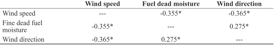
In order to select the appropriate sampling method for the data, it was necessary to determine if the factors were independent (orthogonal), as many sampling methods are
based on this assumption. Wind speed, fine
significantly correlated (Table 2). This
correlation is a likely feature of Santa Ana events, with the associated prevailing conditions of low humidity, high wind speed, and warming. For the purposes of this study, the assumption of stochastic independence was inappropriate; therefore, this research required the use of a sampling method appropriate for correlated inputs.
Sample Generation and Model Evaluation
The recommended sampling method for correlated inputs is replicated Latin Hypercube Sampling (r-LHS) (Saltelli et al. 2004). SIMLAB, a software program for performing uncertainty and sensitivity analysis (Saltelli et
al. 2004), was used to generate 2000 input samples using the r-LHS technique. The Iman and Conover technique was used to control for correlation in the input data by matching the rank-correlation structure of the samples to the empirical data (Iman and Conover 1982). This allows the sampled values to co-vary in a manner that is consistent with the co-variation in the empirical data.
The samples were used as inputs for 2000 HFire model runs, simulating a single event lasting 24 hr in duration, and the total area
burned was extracted from the output files for
each simulation. Fires that reached the boundary of the synthetic landscape were re-run on a larger synthetic landscape. SIMLAB was then used to calculate the importance measures from the distribution of the model Input (units) µ, σ of the data Shapiro-Wilks W for selected transform distributionAssigned
Wind speed (km/hr) 12.83, 6.25 W = 0.9833, p-value = 0.0016
(inverse transform) Normal Fine dead fuel
moisture ( %) 8.59, 4.64 W = 0.9809, p-value = 0.0006 (natural log transform) Normal Wind direction
(degrees) 56.60, 13.04 W = 0.9798, p-value = 0.0003 (square root transform) Normal
Spatial resolution --- --- Uniform
Fuel model --- --- Uniform
X coordinate of
ignition --- --- Uniform
Y coordinate of
ignition --- --- Uniform
Wind speed Fuel dead moisture Wind direction
Wind speed --- -0.355* -0.365*
Fine dead fuel
moisture -0.355* --- 0.275*
Wind direction -0.365* 0.275*
---Table 1. Description of input distributions.
Italicized inputs are trigger factors, designed to allow for modeling choices to be represented as distributions for sampling purposes.
Table 2. Non-parametric correlations, Spearman’s Rho.
outputs. The formulas for estimating the importance measures using r-LHS are
presented in McKay (1996) and Helton and
Davis (2001). In order to assess the stability of the sensitivity estimates, the analysis was repeated using a larger sample size (N = 4000).
reSultS
In the first set of model simulations (N =
2000), 105 ignitions were not successful
because the ignition cell was classified as
unburnable. In the second set of model simulations (N = 4000), 216 ignitions were not successful. The descriptive statistics for the output of the model simulations are presented in Table 3, and the histograms of the outputs are presented in Figures 3a and 3b. The
majority of the observations are at the lower end of the range, with few events in the extreme end of the range, as would be expected for an extreme event. In a visual examination
of the shapes of the modeled fire perimeters, it
was found that simulations with higher wind-speeds resulted in burn perimeters that were generally plume shaped, while the perimeter shapes for simulations in which the wind speed was relatively low are more circular. These
findings are consistent with previous classifications of fire shapes (Albini 1976).
The importance measures for wind speed,
fine dead fuel moisture, and the choice of fuel models were statistically significant for both
sets of simulations (Table 4). Wind speed was
identified as the most influential factor,
accounting for more than 40 % of the variation
in the model output, followed by fine dead fuel
Viable ignitions
Statistics for the total burned area (km2), all simulations (viable ignitions)
Minimum Maximum Mean Standard deviation Simulation set 1
(N = 2000) 1895 (0.0009)0.0000 (3094.62)3094.62 (100.89)95.59 ,, (194.77)190.91 Simulation set 2
(N = 4000) 3784 (0.0009)0.0000 (4658.59)4658.59 (108.32)102.47 (244.33)238.90
Table 3. Descriptive statistics, output of model simulations.
���������������
� ��� ���� ���� ���� ���� ����
� ��� ��� ��� ��� ���� ���� ���� �����
���������������
� ��� ���� ���� ���� ���� ����
� ��� ��� ��� ��� ���� ���� ���� �����
Figure 3a. Histogram of model output, simulation
moisture (less than 15 %), and fuel model (less than 10 %). Wind direction, spatial resolution, and the ignition locations had scores close to zero, indicating that these factors were not
influential and did not have a significant main
effect on the output of the model. The ranking of these factors did not change with the larger sample size.
diSCuSSion
The estimated importance measure for wind speed was more than three times that of
the closest input factor of fine dead fuel moisture. This finding supports the argument that fires burning under Santa Ana conditions
are wind driven events, to the extent that the Rothermel equations in the HFire model
structure represent the physical process of fire spread. In contrast, fine dead fuel moisture
was responsible for less than 15 % of the
variation in simulated fire size. The HFire
model is still being improved upon, and the
identification of wind speed and fine dead fuel moisture as influential factors contributes to
the conceptual validation of the model, as these inputs describe known and expected
influential determinants of fire size. This
research established that the model behaves in a way that conforms to the expectations for the
physical system, increasing the confidence that
can be placed in the model predictions.
This study was framed in terms of
modeling fires in potential Santa Ana
conditions, and the ranking of the input factors could change if a wider range of meteorological
conditions were used. Outside of peak fire season, the fine dead fuel moisture input may have a larger influence, as conditions are more
likely to be unfavorable for burning. The inputs of live herbaceous and woody fuel moistures were not included in this analysis due to the lack of available data. Depending on the seasonal trends, these inputs could be
significant drivers of the model output. To test
this assumption, this analysis should be repeated in a study area where live fuel moistures are regularly monitored. Other options include developing surrogate measures to estimate these inputs from available data or repeating the analysis with synthetic values for live fuel moistures.
The results of this study reflect the influence of the conditions sampled from the
RAWS time series, allowing for a characterization of the sensitivity of the model to each of the climatological inputs separately. Future research will examine methods for sampling the input data in a way that preserves the temporal autocorrelation in the data. One such approach would be to randomly pick a 24 hr series from the data for each replicate. While this method would not provide a separate sensitivity measure for each of the climatological inputs, it would provide a measure of the sensitivity to the diurnal pattern in prevailing conditions. Identifying longer-term patterns may also be useful for simulations that are longer than 24 hr in duration.
The importance measure estimated for fuel model, while even smaller than that of wind
speed or fine dead fuel moisture, was
Wind
speed
Fine
dead fuel
moisture directionWind resolutionSpatial modelFuel X Y Simulation set 1
(N = 2000) 0.4312 0.1448 0.0214 -0.0003 0.0985 0.0210 0.0037 Simulation set 2
(N = 4000) 0.4686 0.1346 0.0408 0.0002 0.0625 0.0090 0.0142
significant. All of the simulations that resulted in fires that were too large for the original
synthetic landscape were simulations using the NFFL fuel maps. The custom models for chaparral shrubs were developed because the NFFL fuel model for chaparral did not represent the more moderate fuel loading found in the chaparral shrublands of the SMM region. The importance of the fuel model input and the questions pertaining to the role
of fuel accumulation in the chaparral fire
regime suggest that this input should be of
concern when modeling fires in chaparral
fuels. Custom fuel models, while costly to
develop, provide site-specific information on important determinants of fire spread. Even under the potential Santa Ana conditions represented in this study, when rates of spread are likely to be maximized, differences in fuel
loading resulted in significantly different spread
predictions. Using NFFL fuel models may
result in over-predicting fire size in most
chaparral landscapes.
The importance measures for spatial resolution in both sets of simulations were close to zero, indicating that changing between 30 m and 100 m resolution has no noticeable
influence on the variability in predicted fire size. Spatial resolution was the least influential
factor for both sets of simulations. The landscape is dominated by chaparral, and the range of possible conditions of chaparral vegetation is condensed into a small number of fuel models. It is perhaps not surprising that the model was insensitive to the way in which this relatively homogeneous landscape was divided. Miller and Yool (2002) suggest the
appropriate resolution for fire modeling
purposes is the resolution that represents the
finest scale of heterogeneity in the landscape.
It would appear that when modeling Santa Ana
fires in this landscape, the 100 m resolution
would be acceptable. Further investigation is needed to identify the threshold resolution that allows for the optimization of predictive
efficiency and accuracy.
The importance measure for wind direction was not a strong driver of model behavior. This could be a result of the synthetic landscape, as the terrain has a directional trending in the canyons that the process of inverting the landscape fails to maintain. The relationship of wind direction to the orientation of the topography could therefore be more
influential than these results would indicate.
Wind direction was also held constant for the simulations and was restricted to the northeast quadrant. These restrictions were considered necessary for representing potential Santa Ana events, when the winds blow persistently from that direction. Representing the full range of wind directions and speeds outside of Santa Ana events could provide insights into the ways in which topography and wind direction and speed may interact in this region.
The importance measures for the coordinates of the potential ignitions locations were very small. The simulations were 24 hr in duration, and the location of a successful
ignition was likely influential during the first few hours and less influential over time. There
were relatively few unburnable ignition locations in this landscape, which led to few simulations in which no area was burned.
The inherent limitations of fire spread
modeling are apparent in this research. This research did not test the assumptions of HFire, the Rothermel (1972) equations, or the Andersen (1983) ellipse model. For example,
the HFire model predicts surface fire spread, and does not model the spread of fire by fire brands or by the ignition of fire gasses. The results of this analysis are specific to the prediction of fire size using the HFire model,
to the chaparral landscape of the Santa Monica Mountains, to the time period of the study, and to potential Santa Ana conditions.
Global Sensitivity Analysis (GSA) is an objective and quantitative method for model evaluation that offers considerable insight for research into physical processes. Given that
ACknowledgeMentS
Thanks are due to H. Johnson for his assistance in the preparation of the figures. This study
was funded in part by the U.S. National Aeronautics and Space Administration, Land Cover Land Use Change Program, Grant No. NAG5-11141.
literAture Cited
Albini, F.A. 1976. Estimating wildfire behavior and effects. USDA Forest Service General
Technical Report INT-30.
Anderson, H.E. 1983. Predicting wind-driven wildland fire size and shape. USDA Forest Service
Research Paper INT-305.
Andrews, P.L. 1989. Application of fire growth simulation models in fire management. Pages
317-321 in: D.C. McIver, H. Auld, and R. Whitewood, editors. Proceedings of the 10th Conference on Fire and Forest Meteorology. Forestry Canada, Ottawa, Canada.
Bessie, W.C., and E.A. Johnson. 1995. The relative importance of fuels and weather on fire
behavior in subalpine forests. Ecology 76: 747-762.
Bevins, C.D., and R.E. Martin. 1978. An evaluation of the slash (I) fuel model of the 1972 National Fire Danger Rating System. USDA Forest Service Research Paper PNW-247.
Bond, W.J., and J.J. Midgley. 1995. Kill thy neighbour: an individualistic argument for the evolution of flammability. Oikos 73(1): 79-85.
Burroughs, L.D. 1991. Forecast guidance for Santa Ana conditions. National Weather Service,
Office of Meteorology Technical Procedures Bulletin 391.
Campolongo, F., A. Saltelli, T. Sorensen, and S. Tarantola. 2000. Hitchhiker’s guide to sensitivityHitchhiker’s guide to sensitivity
analysis. Pages 15-47 in: A. Saltelli, K. Chan, and E. M. Scott, editors. Sensitivity analysis.
John Wiley & Sons, Ltd., Chichester, England. decision-support applications, more attention needs to be paid to incorporating GSA
techniques in other fire modeling studies.
HFire has the ability to stochastically simulate
fire regimes, drawing from a wider range of
historical climatological conditions and
tracking the age of vegetation following fires.
An extension of this analysis will therefore involve conducting a GSA of the model, while
simulating the complexities of a long-term fire
regime at the landscape scale.
Exploring the relative importance of exogenous and stochastic factors (e.g., meteorological variables) as compared to more endogenous and deterministic factors (e.g., plant characteristics) is central to understanding
the fire ecology of many terrestrial ecosystems.
For example, there is support for the idea that
plant flammability may have played an
evolutionary role in some species (Mutch 1970). Given the paucity and the infeasibility
of conducting extensive field experiments,
simulation modeling is one of the few ways we can investigate patterns of plant traits (e.g., Pausas and Lloret 2007) or the degree to which plants may alter their own probabilities of burning at local (e.g., Bond and Midgley 1995) and landscape scales (e.g., Moritz et al. 2005).
Assessing the sensitivities of fire-related
models may thus lead to insights in both
Cruz, M. G., M.E. Alexander, and R.H. Wakimoto. 2003. Definition of a fire behavior model evaluation protocol: a case study application to crown fire behavior models. Pages 48-68 in:
P.N. Omi, and L.A. Joyce, technical editors. Fire, fuel treatments, and ecological restoration: conference proceedings. USDA Forest Service Proceedings RMRS-P-29.
Cukier, R.I., C.M. Fortuin, K.E. Shuler, A.G. Petschek, and J.H. Schaibly. 1973. Study of the sensitivity of coupled reaction systems to uncertainties in rate coefficients I. Theory. The
Journal of Chemical Physics 59: 3873-3878.
Desert Research Institute. 2004. RAWS USA climate archive. Western Regional Climate Center. <http://www.raws.dri.edu/index.html>. Accessed January 5, 2004.
Finney, M.A. 1998. FARSITE: Fire Area Simulator-Model development and evaluation. USDA Forest Service Research Paper RMRS-RP-4.
Hargrove, W.W., R.H. Gardner, M.G. Turner, W.H. Romme, and D.G. Despain. 2000. Simulating
fire patterns in heterogeneous landscapes. Ecological Modelling 135: 243-263.
Helton, J.C., and F.J. Davis. 2001. Latin hypercube sampling and the propagation of uncertainty in analyses of complex systems. Sandia National Laboratories Document 5165.
Iman, R.L., and W.J. Conover. 1982. A distribution-free approach to inducing rank correlation among input variables. Communications in Statistics: Simulation and Computation 11: 311-334.
Keeley, J.E., and C.J. Fotheringham. 1994. Impact of past, present, and future fire regimes on
North American Mediterranean shrublands. Pages 218-262 in: J.M. Moreno, and W.C.
Oechel, editors. The role of fire in Mediterranean-type ecosystems. Springer-Verlag, New
York, USA.
Keeley, J.E., C.J. Fotheringham, and M. Morais. 1999. Reexamining fire suppression impacts on brushland fire regimes. Science 284:1829-1832.
Keeley, J.E., and C.J. Fotheringham. 2001a. Historic fire regime in Southern California
Shrublands. Conservation Biology 15: 1536-1548.
Keeley, J.E., and C.J. Fotheringham. 2001b. History and management of crown-fire ecosystems:
a summary and response. Conservation Biology 15: 1561-1567.
Kourtz, P.H. and W.G. O’Regan. 1971. A model for a small forest fire, to simulate burned and
burning areas for use in a detection model. Forest Science 17: 163-169.
McKay, M.D. 1996. Variance-based methods for assessing uncertainty importance in
NUREG-1150 analyses. Los Alamos National Laboratory LA-UR-96-2695.
Miller, J.D., and S.R. Yool. 2002. Modeling fire in semi-desert grassland/oak woodland: the
spatial implications. Ecological Modelling 153: 229-245.
Minnich, R.A. 1983. Fire mosaics in southern California and northern Baja California. Science 219: 1287-1294.
Minnich, R.A., and C.J. Bahre. 1995. Wildland fire and chaparral succession along the
California-Baja California boundary. International Journal of Wildland Fire 5: 13-24.
Minnich, R.A., and Y.H. Chou. 1997. Wildland fire patch dynamics in the chaparral of southern
California and northern Baja California. International Journal of Wildland Fire 7: 221-248.
Minnich, R.A. 2001. An integrated model of two fire regimes. Conservation Biology 15:
1549-1553.
Morais, M. 2001. Comparing spatially explicit models of fire spread through chaparral fuels: a new algorithm based upon the Rothermel fire spread equation. Thesis, University of
Moritz, M.A. 1997. Analyzing extreme disturbance events: fire in Los Padres National Forest.
Ecological Applications 7(4): 1252-1262.
Moritz, M.A. 2003. Spatiotemporal analysis of controls on shrubland fire regimes: age dependency and fire hazard. Ecology 84(2): 351-361.
Moritz, M.A., J.E. Keeley, E.A. Johnson, and A.A. Schaffner. 2004. Testing a basic assumption of shrubland fire management: how important is fuel age? Frontiers in Ecology and the
Environment 2: 67-72.
Moritz, M.A., M.E. Morais, L.A. Summerell, J.M. Carlson, and J. Doyle. 2005. Wildfires,
complexity, and highly optimized tolerance. Proceedings of the National Academy of Sciences 102(50): 17912-17917.
Mutch, R.W. 1970. Wildland fires and ecosystems - a hypothesis. Ecology 51(6): 1046-1051.
Pausas, J.G., and F. Lloret. 2007. Spatial and temporal patterns of plant functional types under
simulated fire regimes. International Journal of Wildland Fire 16(4): 484–492.
Philpot, C.W. 1977. Vegetative features as determinants of fire frequency and intensity. Pages
12-17 in: H.A. Mooney, and C.E. Conrad, technical coordinators. Proceedings of the
Symposium on the Environmental Consequences of fire and fuel management in
Mediterranean ecosystems. USDA Forest Service General Technical Report WO-3.
Radtke, K., A.M. Arndt, and R.H. Wakimoto. 1982. Fire history of the Santa Monica Mountains.
USDA Forest Service General Technical Report PSW-58.
Rothermel, R.C. 1972. A mathematical model for predicting fire spread in wildland fuels. USDA
Forest Service Research Paper INT-115.
Royston, J.P. 1982. An extension of Shapiro and Wilk’s W test for normality to large samples. Applied Statistics 31: 115-124.
Saltelli, A., F. Campolongo, and E.M. Scott, editors. 2000. Sensitivity analysis. John Wiley & Sons, Ltd., Chichester, England.
Saltelli, A. 2000. What is sensitivity analysis? Pages 3-13 in: A. Saltelli, F. Campolongo, and
E.M. Scott, editors. Sensitivity analysis. John Wiley & Sons, Ltd., Chichester, England. Saltelli, A., S. Tarantola, F. Campolongo, and M. Ratto. 2004. Sensitivity analysis in practice:
guide to assessing scientific models. John Wiley & Sons, Ltd., Chichester, England.
Salvador, R., J. Pinol, S. Tarantola, and E. Pla. 2001. Global sensitivity analysis and scale effects
of a fire propagation model used over Mediterranean shrublands. Ecological Modelling 136:
175-189.
Schroeder, M.J., M. Glovinsky, V.F. Hendricks, F.C. Hood, M.K. Hull, H.L. Jacobsen, R. Kirkpatrick, D.W. Krueger, L.P. Mallory, A.G. Oertel, R.H. Reese, L.A. Serguis, and C.E. Syverson. 1964. Synoptic weather types associated with critical fire weather. US Department
of Commerce, National Bureau of Standards, Institute for Applied Technology AD-449-630.
Trevitt, A.C.F. 1991. Weather parameters and fuel moisture content: standards for fire model
inputs. Pages 157-166 in: N. Cheney and A. Gill, editors. Proceedings of conference on
bushfire modelling and fire danger rating systems. CSIRO Division of Forestry, Yarralumla,
Canberra.
Turanyi, T., and H. Rabitz. 2000. Local methods. Pages 81-100 in: A. Saltelli, F. Campolongo, and E.M. Scott, editors. Sensitivity analysis. John Wiley & Sons, Ltd., Chichester, England. Weise, D.R. 1997. Recent chaparral fuel modeling efforts. Resource Management: the Fire