R E S E A R C H
Open Access
A multi-frame super-resolution method
based on the variable-exponent nonlinear
diffusion regularizer
Baraka Jacob Maiseli
1,2*, Ogada Achieng Elisha
3and Huijun Gao
2Abstract
In this work, the authors have proposed a multi-frame super-resolution method that is based on the diffusion-driven regularization functional. The new regularizer contains a variable exponent that adaptively regulates its diffusion mechanism depending upon the local image features. In smooth regions, the method favors linear isotropic diffusion, which removes noise more effectively and avoids unwanted artifacts (blocking and staircasing). Near edges and contours, diffusion adaptively and significantly diminishes, and since noise is hardly visible in these regions, an image becomes sharper and resolute—with noise being largely reduced in flat regions. Empirical results from both simulated and real experiments demonstrate that our method outperforms some of the state-of-the-art classical methods based on the total variation framework.
Keywords: Super-resolution; Regularization; Image reconstruction; Diffusion
1 Introduction
1.1 Overview of the super-resolution methods
Super-resolution image reconstruction refers to a collec-tion of various image-processing tools used to recon-struct high-resolution images from their corresponding degraded versions ([1–5], and references therein). The term resolution, as used in this work, is the number of pix-els per unit area. Therefore, a high-resolution image with both appreciable subjective and objective qualities has a larger pixel count compared with a low-resolution image.
Humans are naturally inclined to vouch for high-quality images. Perhaps the reason for this inclination is the fact that such images contain more information and, hence, are easier to comprehend and interpret. In machine learn-ing and computer vision tasks, detailed images are useful to accurately and robustly highlight and extract criti-cal features, such as edges and contours. These typicriti-cal examples make super-resolution a vital technology.
*Correspondence: [email protected]
1Department of Electronics and Telecommunication Engineering, College of Information and Communication Technologies, University of Dar es Salaam, P. O. Box 35194, 00255 Dar es Salaam, Tanzania
2Research Institute of Intelligent Control and Systems, Harbin Institute of Technology, 150001 Harbin, China
Full list of author information is available at the end of the article
Super-resolution methods attempt to address the hard-ware limitations for improving image qualities. The advantage of these methods is that they discourage hard-ware modifications to achieve high-resolution images and, thus, are cheap and promote portability. The hardware approach, on the contrary, prompts for changes in the sensor, chip size, and device’s internal circuitry to meet the same goal of the super-resolution process. These hardware changes come at the following costs: (1) the current technology disallows further reduction of the sen-sor’s pixel size (which increases pixel count and, there-fore, improves resolution) as the process may introduce unwanted shot noise that degrades images; (2) increas-ing the chip size, which improves the spatial resolution, raises capacitance that slows down the charge transfer rate; and (3) additional weight due to hardware change may limit particular applications, such as remote sensing or unmanned aerial surveillance.
The methods for solving the super-resolution problem can be put into two groups, namely multi-frame and single-frame. The former group uses a single image to generate its corresponding high-resolution version [6–9]. Despite the extensive review, single-frame-based super-resolution approaches—interpolation (nearest neighbor, bilinear, and bicubic) and example-based [10–13]—tend
to generate unpleasing results due to insufficient amount of input images. For example, interpolation methods are known for producing blurry and aliased images. Besides, example-based approaches are computationally ineffi-cient and may, therefore, be unsuitable for real-time processing. A thorough discussion on single-frame super-resolution methods is beyond the scope of our work. However, for a comprehensive review of this category of methods, we refer interested readers to the works in [7, 8, 14–20]
A multi-frame super-resolution approach—which this paper is based upon—attempts to generate a high-resolution image by fusing some pieces of information from multiple degraded images of the same scene [21–24]. The fundamental premise of this approach is that pairs of similar images are likely to differ by rotations, trans-lations, and/or affine transformations due to (1) shaking of the camera, (2) different capturing and exposure times, and (3) relative motion between camera and scene. We can exploit this additional information to produce a more resolute scene by computing the values of these attributes and using them to align the frames onto a common high-resolution grid. The rest of this work discusses the multi-frame super-resolution methods.
The super-resolution problem is highly ill-posed due to insufficient number of the observed low-resolution frames. A classical approach to address this problem is called regularization. Authors have, therefore, proposed different types of priors.
A classical and, perhaps, popular prior is based on the Tikhonov model [25, 26]. This prior introduces into the restoration problem a smoothness constraint that removes extraneous noise from an image. The weak-ness of the Tikhonov prior is that it tends to destroy edges—an effect that degrades images. Therefore, the prior has captured the interest of many researchers to develop models that simultaneously suppress noise and preserve critical image features: Huber Markov random field (Huber-RMF) [27, 28], edge-adaptive RMF [29, 30], sparse directional [31, 32], and total variation (TV) [33–35].
Of the aforementioned priors, TV has attracted more attention of researchers as it generates results with pleasing objective and subjective qualities. The major weaknesses of the TV model are blocking and staircas-ing effects, false-edge generation near edges, and non-differentiability property at zero—a situation that makes the numerical implementation rather challenging. The TV model was initially applied in image denoising [36]. Later, the model was adapted to other applications: super-resolution [33], MRI medical image reconstruction [37], inpainting [38], and deblurring [39]. In this work, we explore some classical TV-based approaches to address the super-resolution problem.
In 2008, Marquina et al. proposed a convolutional model for a super-resolution problem based on the constrained TV framework [33]. In their work, the authors introduced the Bregman algorithm as an iterative refinement step to enhance the spatial resolution. The results demonstrate that the method generates detailed and sharper images, but blocking and staircasing artifacts are still evident.
In [35], Farsiu and colleagues proposed a bilateral total variation (BTV) prior, which is based on the L1 norm minimization and the bilateral filter regularization func-tional, for a multi-frame super-resolution problem. Their method is computationally inexpensive and robust against errors caused by motion and blur estimations and gen-erates images that are convincingly sharper. However, bilateral filters that the method derives its strengths from are known to introduce artifacts like staircasing and gradi-ent reversal. Additionally, the BTV inadequately addresses the partial smoothness of an image [40]. Besides, the numerical implementation of theL1norm component is challenging as it masks the super-resolution data term.
In [34], Ng et al. applied the TV prior to address the following issues in the super-resolution video reconstruc-tion: noise, blurring, missing regions, compression arti-facts, and motion estimation errors. The authors demon-strated the efficacy of their method in several cases of motions and degradations and provided the experimen-tal results that outperform some other classical super-resolution methods.
Ren et al. proposed a super-resolution method, which is based on the fractional order TV regularization, with a focus to handle fine details, such as textures, in the image [41]. Results show that their approach addresses to some extent the weaknesses of the traditional TV.
In [21], Li et al. attempted to address the drawbacks of the global TV by proposing two regularizing functionals, namely locally adaptive TV and consistency of gradients, to ensure that edges are sharper and flat regions are smoother. The method heavily depends on the gradient details of an image, a feature that may produce pseudo-edges in noisy homogeneous regions. Note that both noise and edges are image features with gradient (or high-intensity) values. As Li’s method is gradient-dependent, it may equally treat both noise and edges, and this may generate unwanted artifacts.
to regularization parameters) and outperforms the Li et al. method. But under severe noise conditions, the Yuan et al. approach fails as it is pixel-unit-based [40].
Recently, Weili et al. proposed an adaptive TV-driven super-resolution method that provides convincing results compared with those generated by the standard TV model [40]. The authors incorporated into the classical super-resolution formulation a feature-sensitive prior that approximates theL1norm near edges, and this helps to efficiently highlight these critical features. In flat regions, the prior approximates theL2norm, thus providing noise removal.
Inspired by the weaknesses of the standard TV and its variants, this work proposes an alternative frame-work based on nonlinear diffusion processes—which have yielded promising results in image-denoising applica-tions [36, 43–47]—to address the super-resolution ill-posedness. Our diffusion-driven prior includes an adap-tive kernel that sensiadap-tively and dynamically updates its value in accordance with the scanned local image fea-tures. That is, the kernel is linear isotropic in flat regions and nonlinear anisotropic near edges. Being locally adap-tive, the model generates more resolute scenes and avoids blocking artifacts inherent in the conventional TV.
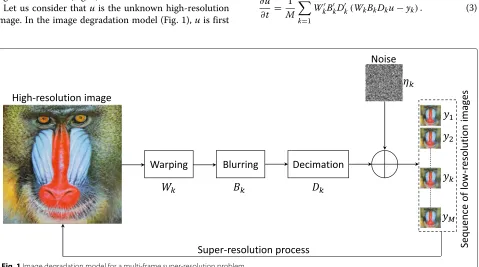
1.2 A classical multi-frame image degradation model Imaging devices, such as cameras, endure unavoidable hardware limitations and influence of external noise. Therefore, an image signal that passes through the imag-ing system usually undergoes degradations before reach-ing its destination (Fig. 1).
Let us consider thatuis the unknown high-resolution image. In the image degradation model (Fig. 1),uis first
acted upon by the warping operator, Wk, which rotates and translates it. Then, the degraded version ofuproceeds to the next stage, where it is blurred by the blurring oper-ator,Bk. In the next stage, the dimension (width×height) of the degraded (warped and blurred)uis decreased by the decimation operator, Dk. Finally, noise (assumed to be additive white Gaussian), ηk, is added as a further image degradation agent. Consequently, a sequence of low-resolution images, {yk}, where k=1, 2, 3,. . .,M is generated. As the model is multi-frame-based, the degra-dation process incorporates a sequence of composite operators—W1B1D1,. . .,WkBkDk,. . .,WMBMDM— which are applied to u to produce y1,. . .,yk,. . .,yM, respectively.
Therefore, we intuitively represent the multi-frame image degradation model by the equation
yk=WkBkDku+ηk (1)
Treatingηkas energy, our objective is to minimize it using theL2norm that is known for its ability to suppress noise. Therefore, the minimization problem becomes
min u
1 2M
M
k=1
yk−WkBkDku2L2()
, (2)
where is the supporting domain of u. Applying the Euler-Lagrange optimization approach, and embedding the resulting solution into a dynamical system, we get
∂u
∂t =
1
M
M
k=1
WkBkDk(WkBkDku−yk). (3)
2 Multi-frame super-resolution process
2.1 Background
The fundamental aim of the super-resolution process is to improve the spatial resolution of an image while sup-pressing unwanted artifacts. A well-known approach to achieve this goal is to incorporate a regularizing potential into the super-resolution energy functional. Therefore, we can reformulate (2) as a variational problem
min u∈BV∩L2()
1 2M M
k=1
(yk−WkBkDku)2dx+
ψ(|∇u|)|∇u|dx
+ λ
2
(u−f) 2dx
,
(4)
where the terms from left are defined as follows: super-resolution or data, regularization potential, and fidelity, respectively. From (4), the coefficient function, ψ(s), simultaneously detects edges and penalizes the norm of the image gradient, and the fidelity term, which contains λ as the regularizing parameter, establishes a trade-off between the evolving image,u, and the initial guess,f.
The parameterized (time-dependent) Euler-Lagrange form of (4) is
∂u
∂t =
1
M
M
k=1
WkBkDk(WkBkDku−yk)
+div
ψ(|∇ u|)
|∇u| +ψ
(|∇u|)∇u
−λ(u−f).
(5)
In [36], Rudin et al. proposedψ(s)=1, and plugging this value into (5) yields
∂u
∂t =
1
M
M
k=1
WkBkDk(WkBkDku−yk)+div
1 |∇u|∇u
−λ(u−f), (6)
which is the multi-frame super-resolution model based on the Rudin-Osher-Fatemi (ROF) regularizing functional. Although the ROF model suppresses noise and effec-tively recovers edges, it has some limitations, as noted by Ogada and colleagues [43]. Firstly, the formulation favors piecewise-constant solutions that result into staircasing effects or even generation of false edges. Secondly, the ROF model tends to reduce contrast in homogeneous or noise-free image regions. Thirdly, the TV diffusion model—despite its anisotropic property—produces a pro-cess that only diffuses in a direction that is orthogonal to the gradients of the image contours. This has a conse-quence of producing blockiness in the results. And lastly, the ROF evolution system contains a|∇1u| component that runs into a spike when |∇u| = 0 in flat regions. To
solve this challenge, the numerical implementations of the model usually incorporate a lifting parameter 0< <1, whereis made too small. That is, the diffusion coefficient in the divergence part of (6) is replaced by |∇u1|+. In our view, this modification limits the accuracy of the results and may even cause instabilities.
Motivated by the weaknesses of the ROF model, Ogada et al. proposed an alternative method for image denois-ing that focuses on selectdenois-ing an appropriate value ofψ(s). Their approach provides a criteria for deciding the nature of ψ(s) in terms of linearity, sub-linearity, and super-linearity. This ensures that the resulting regularizing func-tional is strictly convex and grows linearly. In image-denoising problems, linear growth and convex functionals are known to generate appealing results. Additionally, the authors’ diffusion equation contains the denominator that never collapses to zero even in smooth regions (where |∇u| = 0), thus avoiding the singularity risk like that encountered in the TV problem.
Therefore, Ogada et al. selected a sub-linear growth functional coefficient
ψ(|∇u|)= |∇u|
1+ |∇u|. (7)
Pluggingψ(s)from (7) into (5) gives
∂u
∂t =
1
M
M
k=1
WkBkDk(WkBkDku−yk)+div
2+ |∇u|
(1+ |∇u|)2∇u
−λ(u−f).
(8)
Decomposing (7) intouTT (tangential) anduNN (normal) components yields
∂u
∂t =
1
M
M
k=1
WkBkDk(WkBkDku−yk)+
2+ |∇u|
(1+ |∇u|)2
uTT
+
2 (1+ |∇u|)3
uNN−λ(u−f), (9)
which possesses the diffusion mechanisms in both tan-gential and normal directions to the isophote lines. Fur-thermore, Eq. 9 promotes varying degrees of diffusions depending upon the local image structures, particularly edges and contours.
2.2 Proposed model 2.2.1 Model formulation
The smoothing functional proposed by Ogada et al. [43] produces superior results compared with the Perona-Malik (PM) [44], D-α-PM [45], and total variation [36]. The model has been used for denoising applications. In this work, we have modified the model by integrating into its diffusivity an edge-probing variable exponent that is robust against noise. Furthermore, the modified for-mulation was encapsulated into the classical multi-frame super-resolution model.
Now, we propose a non-variational problem
0=1
M
M
k=1
WkBkDk(WkBkDku−yk)+div ⎛ ⎜ ⎝ 2+
|∇u|
β
1+|∇βu|α(x)
∇u
⎞ ⎟ ⎠
−λ(u−f),
(10)
whereβis a shape-defining parameter and
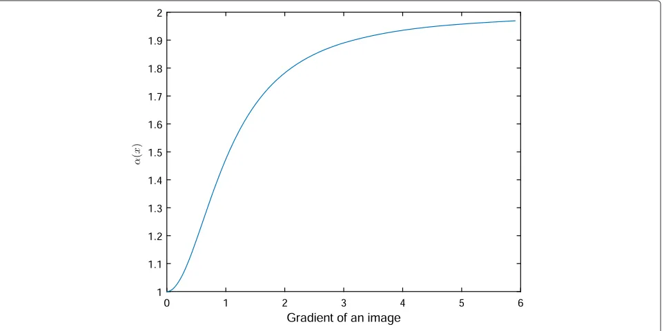
α(x)=2− 1
1+κ|∇(Gσ ∗f)|2 (11)
is an adaptive feature-dependent variable exponent with σ >0 andGσ(x)= 4πσ1 exp
−|x|2 4σ2
(Fig. 2). The authors in [46] found thatσ = 0.50 and 0.0025 < κ < 0.025 produced promising restoration results, and indeed, their findings worked well for our case. Equation 10 is usually solved by embedding it into a dynamical system, which
is then evolved until steady state conditions are attained. Therefore, parameterizing the equation in time yields
∂u
∂t=
1
M
M
k=1
WkBkDk(WkBkDku−yk)+div ⎛ ⎜ ⎝ 2+
|∇u|
β
1+|∇βu|
α(x)∇u ⎞ ⎟ ⎠
−λ(u−f) for (x,t)∈×(0,T),
u(x, 0)=f, x∈, ∂u
∂n=0, (x,t)∂×(0,T),
(12)
which can be implemented in the computer using the appropriate numerical schemes. In this paper, we used the four-point neighborhood explicit scheme to imple-ment (12), as detailed in the later sections.
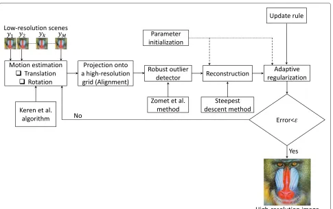
Figure 3 shows the block diagram that implements our model in (12). From the illustration, a sequence of M
frames,y1,y2,. . .,yk,. . .,yM, is first captured by an imag-ing device. Then, the values of the motion parameters (rotations and translations) between{yk+1}k=1,2,...,M and
y1(reference frame) are computed using the Keren et al. algorithm—which is chosen for its reliability, robustness, accuracy, and computational efficiency. Next, the frames are aligned using the computed motion values and pro-jected onto the high-resolution grid. Next, the Zomet et al. method is used to robustly detect outliers in the data. The actual reconstruction is done in the following step, and we used the steepest descent approach for this purpose. Lastly, the proposed regularizing functional is incorpo-rated to address the super-resolution ill-posedness and also to address noise issues in the image. The program’s iteration exit point is determined using theL2error norm
Fig. 3Flow diagram for the proposed framework
u(n)−u(n−1)2 2 u(n)2
2
< ε, (13)
where 0< ε <1 is a tuning constant that determines the final error of the results.
2.2.2 Physical significance and roles ofα(x)
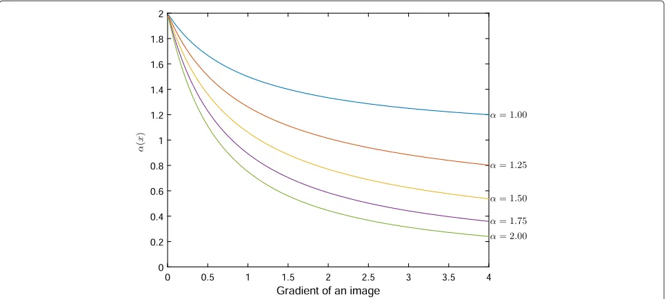
The variable,α ∈[ 1, 2], sweeps values between one and two according to the local features of an image (Fig. 4). From (11), we observe the following cases:
1. In flat regions (|∇(Gσ∗f)| →0),α =1. Substituting this value ofαinto (12) yields
∂u
∂t =
1
M
M
k=1
WkBkDk(WkBkDku−yk)
+div
2+ |∇βu| 1+ |∇βu|∇u
−λ(u−f).
Now, expanding the divergence part of this equation produces
∂u
∂t =
1
M
M
k=1
WkBkDk(WkBkDku−yk)
+div
1 1+ |∇βu|∇u
+ u,
(14)
which combines two regularizing models, namely ROF and isotropic diffusion. Therefore, the formulation can isotropically remove noise in these (flat) regions. Additionally, ifβis carefully tuned, we may preserve weak edges due to the presence of a regularizing component—middle term of (14)—that is similar to that of TV.
2. Near edges (|∇(Gσ∗f)| → ∞),α=2. Thus, Eq. 12 becomes
∂u
∂t =
1
M
M
k=1
WkBkDk(WkBkDku−yk)
+div
⎛ ⎜ ⎝ 2+
|∇u| β
1+ |∇βu|
2∇u ⎞ ⎟ ⎠
Fig. 4Variation of the proposed diffusivity with respect to different values ofα(x)
which contains a regularizing part proposed by Ogada et al. [43]. This formulation helps to suppress noise, avoid diffusion of edges, and enhance the spatial resolution of an image.
3. From the above two cases, I and II, we see thatα(x)
plays another role of segmenting an image into two subregions, namely1(flat regions;α=1) and2
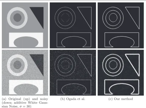
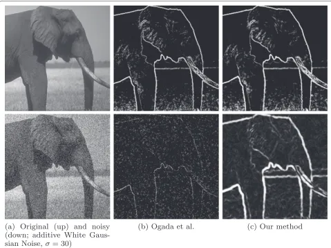
(edges and contours;α=2). Hence,αis an edge-defining variable. An important aspect ofαis that it contains a convolution operator between the Gaussian kernel and the image,Gσ∗f, which helps to suppress noise and other unwanted artifacts— thus detecting useful image features robustly, even under harsh imaging conditions (Figs. 5 and 6).
2.2.3 Properties of the model
To comprehensively understand the (mechanical) prop-erties of our model, consider two orthogonal vectors,
T(x) = (ux,uy)/|∇u| and N(x) = (−uy,ux)/|∇u|, in an image, u, where ux and uy are the first-order partial derivatives of u in the x- and y-direction, respectively, and |∇u| = 0. Additionally, let uTT (tangential) and
uNN (normal) be the second-order partial derivatives of
u, representing diffusions, in the directions ofT andN, respectively. DefininguTTanduNNas
uTT =T∇2uT= 1
|∇u|2
u2xuyy+u2yuxx−2uxuyuxy
and
uNN=N∇2uN= 1
|∇u|2
u2xuxx+u2yuyy+2uxuyuxy
,
whereT = (1/|∇u|)
uy
ux
,N = (1/|∇u|)
ux
uy
, and
∇2u =
uxx uxy
uxy uyy
is the Hessian matrix; Eq. 12 can
compactly be re-written in terms ofuTTanduNNas
∂u ∂t =
1 M
M
k=1
WkBkDk(WkBkDku−yk)+ ⎛ ⎜ ⎝ 2+
|∇u| β
1+|∇u|β α(x) ⎞ ⎟ ⎠uTT
+ ⎛ ⎜ ⎝
1+|∇u|β 2+|∇u|β
+1
−2+|∇u|β
α(x)
1+|∇u|β α(x)+1
⎞ ⎟
⎠uNN−λ(u−f).
(15)
Equation 15 possesses some interesting properties worth noting: in flat regions (|∇u| →0 andα → 1), the equation reduces to
∂u
∂t=
1
M
M
k=1
WkBkDk(WkBkDku−yk)+(CuTT+uNN)−λ(u−f),
(16)
Fig. 5Edge maps of a synthetic image:aoriginal and noisy (white Gaussian noise) image,bimage generated from the Ogada et al. model, and cimage generated using our method
theuTT component that is responsible to preserve edges dominates.
2.3 Numerical implementation
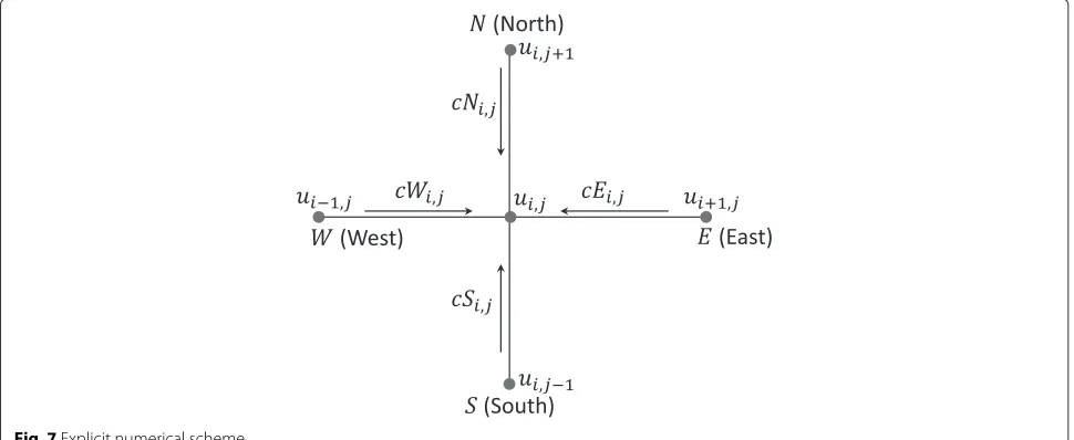
The desire to implement our method using an explicit scheme is attributed to the following reasons: compu-tational efficiency, ability to produce more accurate and appealing results, intuitiveness to be understood and ana-lyzed mathematically, and stability over the time interval defined by the Courant-Friedrichs-Lewy criterion (0 < τ ≤ 0.25) [48]. A significant drawback, however, of explicit schemes is that they are susceptible to instabilities for larger iteration steps.
Now, consider a five-point discretized space
with four directions: north, south, east, and west (Fig. 7). The gradients of ui,j along these direc-tions are, respectively, Ni,j = ui,j+1 − ui,j,Si,j =
ui,j−1−ui,j,Ei,j = ui+1,j−ui,j, andWi,j = ui−1,j−ui,j,
and the corresponding discrete conduction
coeffi-cients from the divergence part of (12) are
cNi,j=
⎛ ⎜ ⎜ ⎝
2+ | N i,j| β
1+| N i,j| β
αi,j
⎞ ⎟ ⎟ ⎠,cSi,j=
⎛ ⎜ ⎜ ⎝
2+ | S i,j| β
1+| S i,j| β
αi,j
⎞ ⎟ ⎟ ⎠,
cEi,j=
⎛ ⎜ ⎜ ⎝
2+| E i,j| β
1+ | E i,j| β
αi,j
⎞ ⎟ ⎟
⎠, and cWi,j=
⎛ ⎜ ⎜ ⎝
2+ | W i,j| β
1+| W i,j| β
αi,j
⎞ ⎟ ⎟ ⎠,
where 0≤i≤Pand 0≤j≤Q;PandQare, respectively, the horizontal and vertical dimensions of ui,j. Following the explicit scheme, we discretize the divergence compo-nent of our formulation as
Fig. 6Edge maps of an elephant image:aoriginal and noisy (white Gaussian noise) image,bimage generated from the Ogada et al. model, andc image generated using our method
From the given discretizations, therefore, the steep-est descent implementation of the regularized super-resolution method in (12) becomes
ui,j(n+1)=ui,j(n)−τRui,j(n)−Mμdiv(i,jn)+Mμλu(i,jn)−fi,j
,
(17)
whereμis a tuning constant and
Ru(i,nj)= 1 M
M
k=1
WkBkDkWkBkDku(i,nj)−(yk)i,j
(18)
is a super-resolution result at the nth iteration. The boundary conditions of (17) are as follows: u(i,0j) =
(yi,j)1 = y1(ih,jh),u(i,0n) = u( n) i,1, u(
n) 0,j = u(
n) 1,j, u(
n) P,j =
u(Pn−)1,j, andui(,nQ)=u(i,nQ)−1
2.4 Performance evaluation of the super-resolution models
To quantitatively evaluate the performance of different super-resolution models, we have used three metrics: peak-signal-to-noise ratio (PSNR) [49, 50], edge similarity (ESIM) [45], and mean structure similarity (MSSIM) [51]. The PSNR measures signal strength relative to noise in the image and is defined by the equation
PSNR=10 log10
2552PQ
u−f22
. (19)
Though widely applied in many image-processing disci-plines, PSNR fails to explain the quality of edges in the restored scenes. Guo et al. addressed this limitation by proposing the metric
Fig. 7Explicit numerical scheme
where EM(u)and EM(f)are, respectively, the edge maps ofu(restored image) andf (initial ideal image), and
PSNR=10 log10PQ|max(f)−min(f)| 2
u−f22
is as proposed in [52]. Moreover, both PSNR and ESIM inadequately address the perceptual qualities of scenes. Wang and colleagues proposed a metric (MSSIM) that explains the statistical inter-dependency of pixels in scenes, thus quantifying their visual appeals [51]. The MSSIM is governed by the equation
MSSIM= (2μuμf +c1)(2σuf +c2) μ2
u+μ2f +c1)(σu2+σf2+c2
, (21)
where the variables, respectively defined foruandfare as follows:μu andμf, mean;σ2
u andσf2, variance; and σuf, covariance. Andc1andc2are stabilizing constants.
3 Experiments
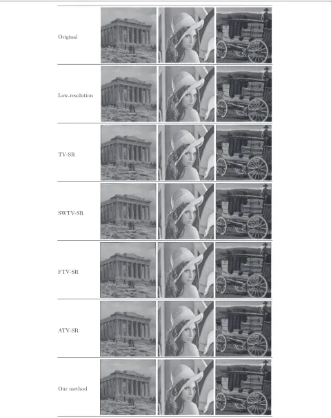
We conducted experiments from both simulated and real environments to test and compare the perfor-mance of the proposed method and some classical super-resolution methods, namely (Total variation) [33], (Spatially weighted total variation) [42], (Fractional order total variation) [41], and (Adaptive total variation) [40]. In the first experiment, we degraded each of the orig-inal high-resolution images of Boat, Bridge, Building, Fish, Goldhill, Lena, Mandrill, and Wheel (http://decsai. ugr.es/cvg/CG/base.htm) (Fig. 8) to generate the corre-sponding sequence of ten low-resolution images. Next, we applied TV-SR, SWTV-SR, FTV-SR, ATV-SR, and the new method to restore the respective original versions of the degraded image sequences (Fig. 9). These procedures were repeated in the second experiment but with the input
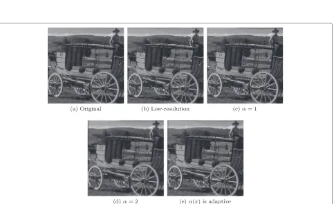
images being the degraded low-resolution video frames of EIA (https://users.soe.ucsc.edu/~milanfar/software/sr-images.html) (Fig. 10). The last experiment tested the effi-cacy of our method for two conditions of the variable exponent,α(x): fixed (α=1 and 2) and adaptive (Fig. 11).
4 Results and discussions
The visual results demonstrate that the proposed method outperforms in several cases compared with some state-of-the-art classical methods (Figs. 9 and 10). Both simu-lated and real experiments show that the new approach generates appealing images that are sharper and detailed. Other methods, such as TV-SR, SWTV-SR, and FTV-SR, reveal obvious artifacts—ringing, blocking, and staircas-ing (Fig. 9). The last experiment proves that the adaptive nature of our formulation helps to preserve useful image features and suppress noise; setting constant the edge-locating variable exponent,α(x), in the proposed model
lowers its performance (Fig. 11). We observed earlier in Section 2.2.2—“Physical significance and roles ofα(x)”— that fixing α to 1 (α = 1), for example, makes the super-resolution problem regularized by both TV and isotropic diffusion, and this promotes edge recovery and noise removal, respectively. The results in the third exper-iment prove this mathematical intuition but also reveal some artifacts that are probably due to fixing α(x), as depicted by Fig. 11c. In Fig. 11e, we observe that adaptively updatingα(x)makes the results appear attractive.
Fig. 8Original high-resolution images:aBoat,bBridge,cBuilding,dFish,eGoldhill,fLena,gMandrill, andhWheel
compared with those from the other methods (Table 2). This finding concurs with the subjective assessments that the proposed method generates images with sharper and stronger edges, which raises the value of the ESIM. In Table 3, the results demonstrate that the new method pro-duces MSSIM values that are larger than those produced by TV-SR, SWTV-SR, FTV-SR, and ATV-SR. This quanti-tative quality assessment justifies the observation that our results are visually appealing (Figs. 9 and 10). Recall that MSSIM favors the human visual system. Furthermore, Table 4 demonstrates that our method offers lower com-putational times—thus making it a suitable choice in tasks that demands parallel computing.
The performance of ATV-SR closely follows that of our method. Subjectively, the results of these two methods are hard to distinguish (Fig. 9; images of Building and Lena; and Fig. 10). However, numerical results indicate that the proposed approach outperforms in several cases (Tables 1, 2, and 3). For the “Wheel” image, however, Table 1 shows that the ATV-SR outperforms our method by a small amount. Also, the ATV-SR is slightly faster than the pro-posed method (Table 4), but the deviation is too small that we may assume the two methods perform equally.
Despite the promising performance, the proposed method suffers from one weakness—it tends to slightly blur the output images. This is probably caused by the low-pass filtering operation of the regularizing functional
or inappropriate estimation of the blur function. More research is thus needed to address the limitation. It is worth noting that the super-resolution results are, how-ever, not only limited to human consumption but also to industrial applications, such as control and automation [53, 54], object detection, and feature extraction. With the proposed method generating promising objective results, we hope that it may as well suit these other disciplines.
5 Conclusions
Fig. 10Super-resolution results of different methods for real video sequences:alow-resolution,bTV-SR,cSWTV-SR,dFTV-SR,eATV-SR, andfour method
Table 1Peak signal-to-noise ratio (PSNR) measurements of different super-resolution methods
Image TV-SR SWTV-SR FTV-SR ATV-SR Our method
Boat 27.73 28.11 28.87 28.05 28.96
Bridge 28.02 29.33 30.15 30.21 31.29
Building 27.43 28.20 27.98 28.74 29.00
Fish 29.12 30.77 30.81 31.00 30.51
Goldhill 28.56 28.90 29.20 30.13 30.78
Lena 27.01 28.21 28.21 29.65 30.71
Mandrill 28.29 29.61 30.33 30.36 30.87
Wheel 29.98 31.05 30.89 31.67 31.59
Mean 28.27 29.27 29.56 29.98 30.46
Table 2Edge similarity (ESIM) measurements of different super-resolution methods
Image TV-SR SWTV-SR FTV-SR ATV-SR Our method
Boat 12.03 12.65 13.09 13.56 13.97
Bridge 13.17 14.00 13.88 14.23 14.78
Building 11.61 12.20 12.09 13.90 13.54
Fish 12.32 13.10 13.71 14.67 14.98
Goldhill 13.54 14.00 13.81 14.01 13.97
Lena 12.70 13.08 13.81 13.56 14.23
Mandrill 13.10 13.45 13.04 14.01 14.53
Wheel 14.01 14.21 13.89 13.22 14.23
Mean 12.81 13.34 13.42 13.90 14.28
Table 3Mean structural similarity (MSSIM) measurements of different super-resolution methods
Image TV-SR SWTV-SR FTV-SR ATV-SR Our method
Boat 0.7812 0.7709 0.7890 0.8102 0.8091
Bridge 0.7901 0.8093 0.8312 0.8200 0.8712
Building 0.7002 0.7856 0.7201 0.7412 0.7554
Fish 0.7812 0.8231 0.8660 0.8700 0.8798
Goldhill 0.7992 0.7085 0.7233 0.7310 0.7620
Lena 0.8441 0.8552 0.8301 0.8400 0.8577
Mandrill 0.8333 0.7898 0.7996 0.8206 0.8790
Wheel 0.7802 0.7790 0.7980 0.7912 0.7993
Mean 0.7887 0.7902 0.7947 0.8030 0.8227
Table 4Algorithmic CPU times (in seconds) of different super-resolution methods
Image TV-SR SWTV-SR FTV-SR ATV-SR Our method
Boat 7.23 8.21 10.19 5.11 6.54
Bridge 8.01 7.40 8.56 4.23 6.35
Building 7.99 7.48 8.32 6.90 5.02
Fish 7.31 6.55 9.02 5.34 5.91
Goldhill 7.87 7.32 8.67 5.40 6.78
Lena 5.12 8.90 10.00 7.98 5.07
Mandrill 9.05 8.92 7.35 4.77 4.33
Wheel 8.69 6.00 7.41 5.93 6.32
In the future, we are contemplating the possibilities of extending our method to other fields, such as in medi-cal imaging. For example, doctors in sonography require high-quality ultrasound images to provide accurate treat-ments to patients. The current instrutreat-ments produce low-quality images that are heavily degraded by multiplicative noise. The problem can be approached in a variety of ways. In the context of the new method, three impor-tant processes that may help to address the problem are (1) modifying the prior to cover multiplicative noise, (2) transforming the model into the three-dimensional space to comprehensively treat the ultrasound images, and (3) implementing the model using more accurate and fast numerical schemes that support real-time parallel com-puting.
Competing interests
The authors declare that they have no competing interests.
Author details
1Department of Electronics and Telecommunication Engineering, College of
Information and Communication Technologies, University of Dar es Salaam, P. O. Box 35194, 00255 Dar es Salaam, Tanzania.2Research Institute of
Intelligent Control and Systems, Harbin Institute of Technology, 150001 Harbin, China.3Department of Mathematics, Egerton University, P. O. Box 536,
00254 Egerton, Nakuru, Kenya.
Received: 23 October 2014 Accepted: 24 June 2015
References
1. B Goldlücke, M Aubry, K Kolev, D Cremers, A super-resolution framework for high-accuracy multiview reconstruction. Int. J. Comput. Vis.106(2), 172–191 (2014)
2. S Park, M Park, M Kang, Super-resolution image reconstruction: a technical overview. Signal Process Mag. IEEE.20(3), 21–36 (2003) 3. B Maiseli, C Wu, J Mei, Q Liu, H Gao, A robust super-resolution method
with improved high-frequency components estimation and aliasing correction capabilities. J. Franklin Institute.351, 513–527 (2014) 4. RS Babu, KS Murthy, A survey on the methods of super-resolution image
reconstruction. Int. J. Comput. Appl.15(2), 1–6 (2011)
5. K Nasrollahi, TB Moeslund, Super-resolution: a comprehensive survey. Mach. Vis. Appl.25, 1423–1468 (2014)
6. Y Zhou, Z Tang, X Hu, Fast single image super resolution reconstruction via image separation. J. Netw.9(7), 1811–1818 (2014)
7. Y Tang, P Yan, Y Yuan, X Li, Single-image super-resolution via local learning. Int. J. Mach. Learn. Cybernet.2, 15–23 (2011)
8. W Wu, Z Liu, X He, W Gueaieb, Single-image super-resolution based on Markov random field and contourlet transform. J. Electronic Imaging.
20(2), 023005–023005 (2011)
9. KI Kim, Y Kwon, Single-image super-resolution using sparse regression and natural image prior.Pattern Anal. Mach. Intell. IEEE Trans.32(6), 1127–1133 (2010)
10. WT Freeman, TR Jones, EC Pasztor, Example-based super-resolution. Comput. Graphics Appl IEEE.22(2), 56–65 (2002)
11. K Zhang, X Gao, X Li, D Tao, Partially supervised neighbor embedding for example-based image super-resolution. Selected Topics Signal Process IEEE J.5(2), 230–239 (2011)
12. C Kim, K Choi, JB Ra, Example-based super-resolution via structure analysis of patches. Signal Process Lett. IEEE.20(4), 407–410 (2013) 13. Z Xiong, D Xu, X Sun, F Wu, Example-based super-resolution with soft
information and decision. Multimedia IEEE Trans.15(6), 1458–1465 (2013) 14. CY Yang, JB Huang, MH Yang, inComputer Vision–ACCV 2010. Exploiting
self-similarities for single frame super-resolution (Springer Queenstown, New Zealand, 2011), pp. 497–510
15. O Mac Aodha, ND Campbell, A Nair, GJ Brostow, inComputer Vision–ECCV 2012. Patch based synthesis for single depth image super-resolution (Springer Florence, Italy, 2012), pp. 71–84
16. X Gao, K Zhang, D Tao, X Li, Joint learning for single-image
super-resolution via a coupled constraint. Image Process IEEE Trans.21(2), 469–480 (2012)
17. J Li, X Peng, inInformation Science and Technology (ICIST) 2012
International Conference on. Single-frame image super-resolution through gradient learning (IEEE Hubei, 2012), pp. 810–815
18. K Zhang, X Gao, D Tao, X Li, Single image super-resolution with non-local means and steering kernel regression. Image Process IEEE Trans.21(11), 4544–4556 (2012)
19. M Yang, Y Wang,A self-learning approach to single image super-resolution, vol. 15. (IEEE Transactions on Multimedia, 2013), pp. 498–508
20. K Zhang, X Gao, D Tao, X Li, Single image super-resolution with multiscale similarity learning. Neural Netw Learn. Syst. IEEE Trans.24(10), 1648–1659 (2013)
21. X Li, Y Hu, X Gao, D Tao, B Ning, A multi-frame image super-resolution method. Signal Processing.90(2), 405–414 (2010)
22. BJ Maiseli, Q Liu, OA Elisha, H Gao, Adaptive Charbonnier superresolution method with robust edge preservation capabilities. J. Electronic Imaging.
22(4), 043027–043027 (2013)
23. B Maiseli, O Elisha, J Mei, H Gao,Edge preservation image enlargement and enhancement method based on the adaptive Perona–Malik non-linear diffusion model, vol. 8. (IET Image Processing, 2014), pp. 753–760 24. XD Zhao, ZF Zhou, JZ Cao, L Ren, GS Liu, H Wang, DS Wu, JH Tan,
Multi-frame super-resolution reconstruction algorithm based on diffusion tensor regularization term. Appl. Mech. Mater.543, 2828–2832 (2014) 25. M Elad, A Feuer, Restoration of a single superresolution image from
several blurred, noisy, and undersampled measured images. Image Process IEEE Trans.6(12), 1646–1658 (1997)
26. N Nguyen, P Milanfar, G Golub, A computationally efficient superresolution image reconstruction algorithm. Image Process IEEE Trans.10(4), 573–583 (2001)
27. D Rajan, S Chaudhuri, An MRF-based approach to generation of super-resolution images from blurred observations. J. Math. Imaging Vis.
16, 5–15 (2002)
28. A Kanemura, Si Maeda, S Ishii, Superresolution with compound Markov random fields via the variational EM algorithm. Neural Netw.22(7), 1025–1034 (2009)
29. KV Suresh, GM Kumar, A Rajagopalan, Superresolution of license plates in real traffic videos. Intell. Transportation Syst. IEEE Trans.8(2), 321–331 (2007)
30. W Zeng, X Lu, A generalized DAMRF image modeling for superresolution of license plates. Intell. Transport. Syst. IEEE Trans.13(2), 828–837 (2012) 31. S Mallat, G Yu, Super-resolution with sparse mixing estimators. Image
Process IEEE Trans.19(11), 2889–2900 (2010)
32. W Dong, D Zhang, G Shi, X Wu, Image deblurring and super-resolution by adaptive sparse domain selection and adaptive regularization. Image Process IEEE Trans.20(7), 1838–1857 (2011)
33. A Marquina, SJ Osher, Image super-resolution by TV-regularization and Bregman iteration. J. Scientific Comput.37(3), 367–382 (2008) 34. MK Ng, H Shen, EY Lam, L Zhang, A total variation regularization based
super-resolution reconstruction algorithm for digital video. EURASIP J. Adv. Signal Process.2007(2007). doi:10.1155/2007/74585
35. S Farsiu, MD Robinson, M Elad, P Milanfar, Fast and robust multiframe super resolution. Image Process IEEE Trans.13(10), 1327–1344 (2004) 36. LI Rudin, S Osher, E Fatemi, Nonlinear total variation based noise removal
algorithms. Physica D: Nonlinear Phenomena.60, 259–268 (1992) 37. F Knoll, K Bredies, T Pock, R Stollberger, Second order total generalized
variation (TGV) for MRI. Magnet Resonance Med.65(2), 480–491 (2011) 38. P Getreuer, Total variation inpainting using split Bregman. Image Process
Line.2, 147–157 (2012)
39. A Bini, M Bhat, A nonlinear level set model for image deblurring and denoising. Visual Comput.30(3), 311–325 (2014)
40. W Zeng, X Lu, S Fei,Image super-resolution employing a spatial adaptive prior model, vol. 162, (2015), pp. 218–233
41. Z Ren, C He, Q Zhang, Fractional order total variation regularization for image super-resolution. Signal Process.93(9), 2408–2421 (2013) 42. Q Yuan, L Zhang, H Shen, Multiframe super-resolution employing a
spatially weighted total variation model. Circ. Syst. Video Technol. IEEE Trans.22(3), 379–392 (2012)
Publishing Corporation 410 Park Avenue 15th Floor, #287 pmb New York, NY 10022 USA, 2014)
44. P Perona, J Malik, Scale-space and edge detection using anisotropic diffusion. Pattern Anal. Mach. Intell. IEEE Trans.12(7), 629–639 (1990) 45. Z Guo, J Sun, D Zhang, B Wu, Adaptive Perona–Malik model based on the
variable exponent for image denoising. Image Process IEEE Transa.21(3), 958–967 (2012)
46. S Levine, Y Chen, J Stanich, Image restoration via nonstandard diffusion. Duquesne University, Department of Mathematics and Computer Science Technical Report :04–01 (2004)
47. J Weickert,Anisotropic diffusion in image processing, Volume 1. (Teubner Stuttgart, 1998)
48. R Courant, K Friedrichs, H Lewy, On the partial difference equations of mathematical physics. IBM J. Res. Dev.11(2), 215–234 (1967) 49. Z Wang, AC Bovik, Mean squared error: love it or leave it? A new look at
signal fidelity measures. Signal Process Mag. IEEE.26, 98–117 (2009) 50. A Tanchenko, Visual-PSNR measure of image quality. J. Visual Commun.
Image Representation.25(5), 874–878 (2014)
51. Z Wang, AC Bovik, HR Sheikh, EP Simoncelli, Image quality assessment: from error visibility to structural similarity. Image Process IEEE Trans.13(4), 600–612 (2004)
52. S Durand, J Fadili, M Nikolova, Multiplicative noise removal using L1 fidelity on frame coefficients. J. Math. Imaging Vis.36(3), 201–226 (2010) 53. S Yin, X Li, H Gao, O Kaynak,Data-based techniques focused on modern
industry: an overview, vol. 62. (IEEE Transactions on Industrial Electronics, 2015), pp. 657–667
54. S Yin, SX Ding, X Xie, H Luo, A review on basic data-driven approaches for industrial process monitoring. IEEE Trans. Industrial Electronics.61(11), 6418–6428 (2014)
Submit your manuscript to a
journal and benefi t from:
7Convenient online submission 7Rigorous peer review
7Immediate publication on acceptance 7Open access: articles freely available online 7High visibility within the fi eld
7Retaining the copyright to your article