R E S E A R C H
Open Access
A study on different experimental
configurations for age, race, and gender
estimation problems
Pierluigi Carcagnì
*, Marco Del Coco, Dario Cazzato, Marco Leo and Cosimo Distante
Abstract
This paper presents a detailed study about different algorithmic configurations for estimating soft biometric traits. In particular, a recently introduced common framework is the starting point of the study: it includes an initial facial detection, the subsequent facial traits description, the data reduction step, and the final classification step. The algorithmic configurations are featured by different descriptors and different strategies to build the training dataset and to scale the data in input to the classifier. Experimental proofs have been carried out on both publicly available datasets and image sequences specifically acquired in order to evaluate the performance even under real-world conditions, i.e., in the presence of scaling and rotation.
Keywords: LBP, CLBP, HOG, SWLD, Digital signage, Audience measurement
1 Introduction
Biometrics have attracted much interest in the last decade, for the high number of applications they can have in industrial and academic fields [1].
Recently, soft biometrics have been clearly defined in [2] as a set of traits providing information about an individ-ual, even though the lack of distinctiveness and perma-nence does not allow to authenticate individuals. These traits can be either continuous (e.g., height and weight) or discrete (e.g., gender, eye color, ethnicity, etc.).
Soft biometrics have widespread use for security, digital signage, domotics (the study of the realization of an intel-ligent home environment), home rehabilitation, artificial intelligence, and so on. Even socially assistive technologies are a new and emerging field where these solutions could considerably improve the overall human-machine interac-tion level (for example with autistic individuals [3], as well as with people with dementia [4] and, generally, for elderly care [5]).
In the last few decades, computer vision, as well as other information science fields, have largely investigated the problem of the automatic estimation of the main soft
*Correspondence: [email protected]
Institute of Applied Sciences and Intelligent Systems, National Research Council of Italy c/o Dhitech scarl, Via Monteroni, 73100 Lecce, Italy
biometric traits by means of mathematical models and ad hoc coding of the visual images. In particular, the automatic estimation of gender, race, and age from facial images are among the most investigated issues, but there is still a lot of open challenges especially for race and age. The extraction of this kind of information is not trivial due to the ambiguity related to the anatomy of each indi-vidual and his lifestyle. In particular, in race recognition, the somatic traits of some population could be not well defined: for example, one person may exhibit some fea-tures more than another one. Similar considerations apply to age estimation, where the appearance of biological age could be very different from the chronological one.
The recent efforts led to a shared and effective frame-work that includes an initial facial detection, a subse-quent description of facial traits, a data reduction step (optional), and a final classification step. The effective-ness of this framework has been already experimentally proved in [6] where some key aspects (like the data reduction strategy) were definitively clarified. Neverthe-less, in the literature, there is no comprehensive study that investigates which methods and techniques are best suited to address the involved algorithmic steps, i.e., to give evidence of the best configuration of the aforemen-tioned framework in terms of facial descriptors, learning strategies, and numerical scale of the data in input to
the classifier. Moreover, the performance of the frame-work under real world conditions (even in the presence of scaling and rotation of the head) has not been fully addressed. To fill this gap, in this paper, a detailed study about different algorithmic configurations for estimating soft biometric traits is presented. First, some of the most used facial descriptors for gender, race, or age estimation were selected, and then, their performances, by using each of them into the considered framework, were compared. This experimental phase was carried out on publicly avail-able face datasets, considering different working strategies (i.e., the balancing/unbalancing of the training dataset and the numerical range of the input measurements). Then, the best configuration was thoroughly tested, for all the involved descriptors, on ad hoc image sequences acquired in a real environment and also considering changes of the head in both position and scale.
The considered feature descriptors were those that, from a detailed study of the literature (reported in next session), demonstrated to be the best suited for encod-ing the biometric traits both in terms of accuracy and computational efficiency. In particular, this paper inves-tigates local binary pattern (LBP) [7, 8], compound local binary pattern (CLBP) [9] (both oriented to texture analy-sis), histogram of oriented gradient (HOG) [10] (designed for shape analysis), and one descriptor that represents a trade-off between the two aspects: Weber local descriptor (WLD) [11]. They were evaluated in a consolidated frame-work where data reduction is achieved by Fisher linear discriminant analysis (LDA) [12] and then support vec-tor machines (SVMs) are used both for classification (race and gender) and regression (for age estimation). SVM [13, 14] is one of the most exploited method in dis-crete biometric estimation problems whose superiority has been well proved in preliminary studies about the performance of different classifiers [15, 16].
Briefly, the main contributions of this paper are as follows:
1. A survey of existing methods and techniques addressing soft biometric issues, in order to discover the most affordable framework;
2. An exploration of various configurations about the components of the framework, in terms of learning strategies and numerical scale of data in input to the classifier, in order to discover the best way to exploit it in soft biometric contexts;
3. The evaluation of the performances of the
aforementioned framework when using the different descriptors also in real-world conditions (even in the presence of scaling and head rotation).
The remainder of the paper is organized as fol-lows: Section 2 discusses the existing literature for the
considered biometric issues; in Section 3, the framework for age, gender, and race classification is explained in detail while in Section 4, the experimental setup and results are detailed and discussed. Finally, conclusions and future developments are discussed in Section 5.
2 Related works
The study of algorithms investigating soft biometric traits has attracted considerable interest in the last two decades. In the following subsections, the most relevant solutions for each specific addressed problem (such as gender, race, and age) are reported.
2.1 Gender
Automatic gender recognition is the most debated soft biometric issue and, over the years, many approaches have been proposed in literature. Three exhaustive sur-veys can be found in [17, 18] and [19]. Early studies mainly exploited geometrical-based methods; Brunelli and Poggio [20] computed 18 distances between face key points and then they used them to train a hyper basis function network classifier, whereas 22 normal-ized vertical and horizontal fiducial distances starting from 40 manually extracted facial points were used by Fellous in [21]. This approach has been recently reassessed by Mozzafari et al. [22] who used the aspect ratio of face ellipse as geometric feature to reinforce appearance information.
In the early 2000s, appearance-based methods were introduced in their basic form, i.e., by evaluating the pixel intensity values. With these approaches, the amount of useless data is a crucial issue that Abdi et al. [23] man-aged by a principal components analysis (PCA), whereas Tamura et al. [24] investigated gender estimation capa-bilities from pixel intensity on small-sized facial images. Conversely, the most interesting progress was made with the introduction of the LBP descriptor [7] to encode infor-mation about facial appearance. LBP, in combination with SVM, was used by Lian and Lu [25] for multi-view gen-der classification. It was also exploited by Yang and Ai [26] to classify age, gender, and ethnicity. LBP descriptor was employed in [27] in combination with intensity and shape features to get a multi-scale fusion approach, while Ylioinas et al. [28] combined it with contrast information in order to achieve a more robust classification. To extract the most discriminative LBP features, Shan [29] proposed an AdaBoost selection method and many other variants have also been proposed to get more informative features, e.g., local Gabor binary mapping pattern [30, 31] and local directional pattern [32].
shape models (ASM) were exploited by Gao and Ai in [36]; Saatci and Town [37] used some features extracted by trained active appearance models (AAM) [38] and supplied them to SVM classifiers arranged into a cas-cade structure in order to optimize overall recognition performance.
Scale invariant feature transform (SIFT) presents some advantages in terms of invariance to image scaling, trans-lation, and rotation; accordingly, the use of SIFT does not require preprocessing stage, like accurate face alignment. Demirkus et al. [39] exploited these characteristics using a Markovian classification model, and Wang et al. [40] extracted SIFT descriptors at regular image grid points and combined them with global shape contexts of the face, adopting AdaBoost for classification.
The desire to imitate nature recently led researches to adopt Gabor filter to copy the cortex view system. In [41], 2-D Gabor wavelets at different scales and eight orienta-tions were extracted, selected by AdaBoost and classified by a Fuzzy SVM that indicated the degree of one’s per-son face belonged to female/male faces. Scalzo et al. [42] extracted a large set of features using Gabor and Laplace filters which were fused by genetic algorithms. Gabor filters, also inspired the modeling of biological inspired features (BIF) employed by Meyers and Wolf [43] for face processing. Finally, Guo et al. in [34] demonstrated that the performance of the gender recognition is affected significantly by human age.
2.2 Race
In the last few years, the race estimation problem has been addressed through several approaches. In [44], the skin color, the forehead area, and the lip color were used in order to estimate ethnicity, whereas in [45] kernel class-dependent feature analysis was used in combina-tion with skin color features to tackle the problem of ethnicity estimation on large scale face databases. PCA was introduced in [46] to perform two-class (Myanmar vs. non-Myanmar) race classification and in [47] to clas-sify, using a feed forward neural network, three (Arabic, Asian, and Caucasian) races. The problem of classifying people into Asian and non-Asian was addressed in [48]. The authors used PCA for features generation and inde-pendent component analysis for features extraction. Final classification was performed by means of a combination of different SVM classifiers. In [49], Gabor features were extracted from facial parts taking into account displace-ment issues, and SVM was then employed as classifier. A method, referred to as local gradient Gabor pattern, was proposed in [50]. It is based on the use of gradient infor-mation on Gabor-transformed images, demonstrating its effectiveness with images having variations in expression and illumination. In [51], faces were represented using elastic graphs labelled with 2-D Gabor wavelet features,
and the system was trained from examples to classify faces on the basis of sex, race, and expression using linear discriminant analysis. In [52], the problem of large-scale ethnicity estimation under variations of gender and age was addressed. Biologically inspired features, with man-ifold learning, were used to represent faces for ethnicity estimation demonstrating their robustness and high eth-nicity classification accuracies within same-gender and same-age groups. An interesting analysis of age estima-tion performance under variaestima-tions across race and gender was proposed in [53–55], whereas in [56], a joint estima-tion framework capable to deal with the mutual influence of gender, race, and age was introduced.
In [57], a fusion scheme for ethnicity estimation that combines Haar wavelet-based global features and uniform LBP-based local features was presented. The dimension-ality of the obtained vector of features was reduced by means of PCA, and a K-nearest neighbor classifier was employed as final step. LBP histogram (LBPH) features were extracted in [26] to estimate Asian and non-Asian ethnicity by means of AdaBoost classifiers. LBP was also used in [58] and then fused with Weber local descriptors through concatenation to produce a more powerful set of features to be supplied to a minimum distance classi-fier for the final race estimation. WLD histograms were employed in [59] demonstrating that they outperform PCA-based holistic methods. Race estimation was also addressed in [60] where a LDA representation was devel-oped under the Bayesian statistical decision framework: the task was formulated as a two-category classification problem to classify between Asian or non-Asian subjects. Finally, in [61], two of the above problems (the estimation of gender and race) were faced using facial imagery. In particular, the examination of the 3-D meshes of the face, without any associated texture or photographic informa-tion, was performed.
2.3 Age
the face anthropometry, the science of measuring human face size and proportions: 57 facial key points were used to measure distances of interest and a model for age evaluation was provided. Unfortunately, these approaches were proved to be unreliable for the evaluation of age in adult people but sufficiently discriminative just in the growing age.
A more interesting approach was proposed by Lanitis et al. [67] who introduced an aging function (valid for younger ages) related to the features vector of raw AAM parameters [38]. In a similar way, Liu et al. [68] pro-posed, in recent years, the use of AAM in association with PCA and an SVM classifier experiencing interesting results.
An innovative prospective was instead given by Geng et al. [69] who used an EM-like iterative learning algo-rithm to model the incomplete aging pattern extracted by observing the same individual at different ages. A similar approach, but oriented to find a common pattern among different individuals, was proposed in [70] and [71].
Another major trend, in the aging-related facial fea-tures extraction, focuses on the use of an appearance model that can be handled as a global or local fea-tures extraction issue. The first attempts in this research line were in [72, 73] where texture and shape features were jointly exploited to increase the descriptor robust-ness in order to estimate the human ages through a multiple-group classification scheme with 5-year inter-vals taking also advantage from the gender knowledge (since the aging patterns are different for males and females). Successively, the interest in appearance-based descriptors arose exponentially and LBP was used for appearance features extraction in an automatic age esti-mation system proposed in [74], whereas some variants were proposed and tested in [75, 76]. Gabor features were also tried for age estimation purposes [77] demon-strating their discriminative power. BIF [78, 79] in aging problems were also explored by Guo et al. in [80] and Lian et al. in [81].
Recently, many other approaches were investigated. Lou et al. in [82] tested the use of HAAR features and SVM for a human-robot interaction application based on the age estimation. A learning-based encoding was proposed by Alnajar et al. in [83] showing that an image encoding based on the learning feedback can improve the over-all estimation accuracy. One of the most recent works exploited the information derived from the dynamic of facial landmarks in video sequences [84].
An approach to gender and age classification prob-lems from video sequences, which encodes and exploits the correlation between the face images through man-ifold learning, was proposed in [85]. Finally, in [86], a study of the influence of demographic appearance in face recognition was proposed: gender (male and female),
race/ethnicity (Black, White, and Hispanic), and age group (18–30, 30–50, and 50–70 years old) were taken into account comparing six different solutions.
3 System overview
In this section, the common framework used to address different soft biometric issues (gender, age, and ethnic-ity) is introduced: it is able to automatically extract soft biometrics information from generic video sequences through a complex pipeline of operational blocks. The pipeline is schematically depicted in Fig. 1: the first step is devoted to the detection and normalization of faces in the running image. The outcomes of the first step are the input of the following step, aimed at extracting a new rep-resentation of facial regions, depending on the selected descriptor. In particular LBP, HOG, SWLD, and CLBP are considered in this paper.
The set of extracted features is then projected (through LDA) on a more suited subspace where it is possible to include most of the initial discriminative information in a reduced number of variables. Finally, the retained variables are given as input to the learned SVM classi-fier that assures efficiency both in terms of accuracy and computational load.
The following subsections will detail each step giv-ing information, also, about the family of compargiv-ing descriptors.
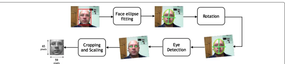
3.1 Face detection and normalization
In this step, human faces are detected in the input images and then a normalization operation is done. Normaliza-tion is a fundamental preprocessing step since the subse-quent algorithms work better if they can evaluate input faces with predefined size and pose. The face detection is performed by means of the well-known Viola-Jones [87] approach (which combines increasingly more complex classifiers in a cascade) based detectors for face and head-shoulder (which helps to handle low resolution images) detection. Whenever a face is detected, the face normal-ization is carried out as follows: the system, at first, fits an ellipse to the face blob (exploiting facial features color models) in order to rotate it to a vertical position and hence a Viola-Jones-based eye detector searches the eyes. Finally, eye positions, if detected, provide a measure to crop and scale the frontal face candidate to a standard size of 65×59 pixels. The above face registration procedure is schematized in Fig. 2.
Fig. 1Block diagram of the estimation framework: the raw frames are processed in order to obtain a reliable class estimation of the people in the scene
3.2 Features extraction
After the face detection and normalization step, a suit-able family of descriptors has to be chosen in order to build a vector of features able to encode distinctive local structures in the facial region. The selected descriptors should be highly distinctive, i.e., with low probability of mismatch but, at the same time, their computational load and sensibility to the noise, such as changes in illu-mination, scaling, rotation, skew, etc., have to be kept low. The choice of the best family of descriptors is not straightforward: many different approaches have been introduced and effectively used in different academic fields, but the best strategy in the context of soft biomet-ric estimations does not emerge from the literature. For this reason, in this paper, four different data descriptors have been considered and experimentally compared. For
each of them, a short description is given in the following subsections.
3.2.1 LBP
LBP is a local feature widely used for texture description in pattern recognition. The original LBP assigns a label to each pixel. Each pixel is used as a threshold and com-pared with its neighbor. If the neighbor is higher, it takes value 1; otherwise it takes value 0. Finally, the thresholded neighbor pixel values are concatenated and considered as a binary number that becomes the label for the central pixel. A graphical representation is shown in Fig. 3a and defined as follows:
LBPP,R(xc)= P−1
p=0
u(xp−xc)2p (1)
Fig. 3LBP descriptor: labeling procedure (a) and spatial histogram concatenation (b)
whereu(y)is the step function,xpthe neighbor pixels,xc the central pixel,P the number of neighbors, andR the radius. To account for the spatial information, the image is then divided into regions. LBP is applied to each sub-region, and an histogram of L bins is generated from the pixel labels. Then, the histograms of different regions are concatenated in a single higher dimensional histogram, as represented in Fig. 3b.
3.2.2 CLBP
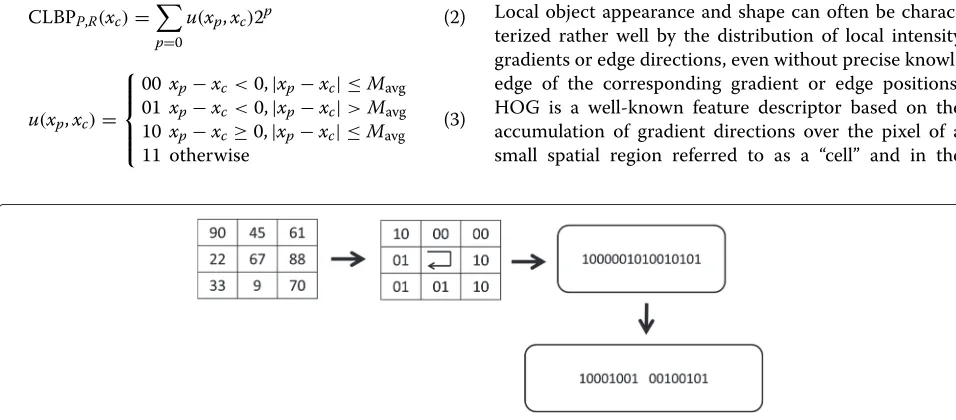
CLBP is an extension of the LBP descriptor designed essentially for facial expression recognition [9]. Compared to LBP, CLBP encodes the sign of the differences between the center pixel and itsP neighbors as well as the mag-nitude of the differences. This involves a code length of 2P-bit:P for the signs andPfor the magnitudes (Fig. 4). That is,
CLBPP,R(xc)= P−1
p=0
u(xp,xc)2p (2)
u(xp,xc)= ⎧ ⎪ ⎪ ⎨ ⎪ ⎪ ⎩
00xp−xc<0,|xp−xc| ≤Mavg 01xp−xc<0,|xp−xc|>Mavg 10xp−xc≥0,|xp−xc| ≤Mavg 11 otherwise
(3)
where Mavg is the average magnitude of the difference between the center and the neighbors values.
As an example, considering a neighborhood 3×3, the CLBP encodes a vector of 16 bits long provided by 8 bits for the magnitude an 8 bits for the sign patterns. In par-ticular, the two patterns are built by concatenating the corresponding values of the bit sequence (1, 2, 5, 6, .., 2P -3, 2P-2) and (3, 4, 7, 8, .., 2P-1, 2P) of the original CLBP code. In this way, two images are obtained from the orig-inal one, by replacing each pixel with the two sub-CLBP patterns. A feature representation of the original image is then obtained by concatenating the histograms of the two images. In order to account for spatial information, the image is firstly divided into sub-regions and then CLBP is applied to each of them, similarly to the spatial LBP operator.
3.2.3 HOG
Local object appearance and shape can often be charac-terized rather well by the distribution of local intensity gradients or edge directions, even without precise knowl-edge of the corresponding gradient or knowl-edge positions. HOG is a well-known feature descriptor based on the accumulation of gradient directions over the pixel of a small spatial region referred to as a “cell” and in the
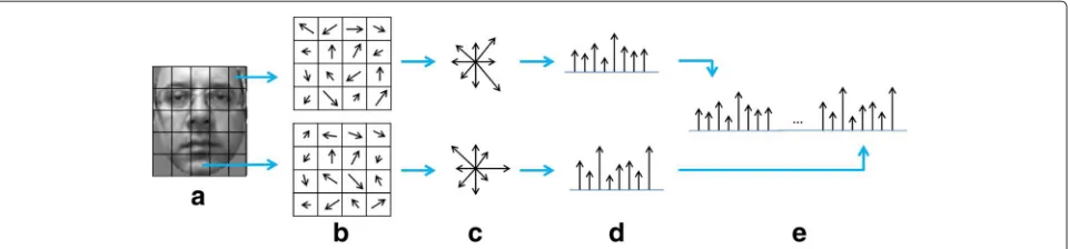
consequent construction of a 1-D histogram. Although HOG has many precursors, it has been used in its mature form in scale invariant features transformation [89] and widely analyzed in human detection by Dalal and Triggs [10]. This method is based on evaluating well-normalized local histograms of image gradient orientations in a dense grid. LetLbe the image to analyze. The image is divided into cells (Fig. 5a) of sizeN×Npixels, and the orientation θof each pixelx=(xx,xy)is computed (Fig. 5b) by means of the following relationship:
θ(x)=tan−1L(xx,xy+1)−L(xx,xy−1)
L(xx+1,xy)−L(xx−1,xy)
(4)
The orientations are accumulated in an histogram of a predetermined number of bins (Fig. 5c, d). Finally, his-tograms of each cell are concatenated in a single spatial HOG histogram (Fig. 5e). In order to achieve a better invariance to noise, it is also useful to contrast-normalize the local responses before using them. This can be done by accumulating a measurement of local histogram energy over larger spatial regions, named blocks, and using the results to normalize all of the cells in the block. The normalized descriptor blocks will represent the HOG descriptor.
3.2.4 Spatial WLD
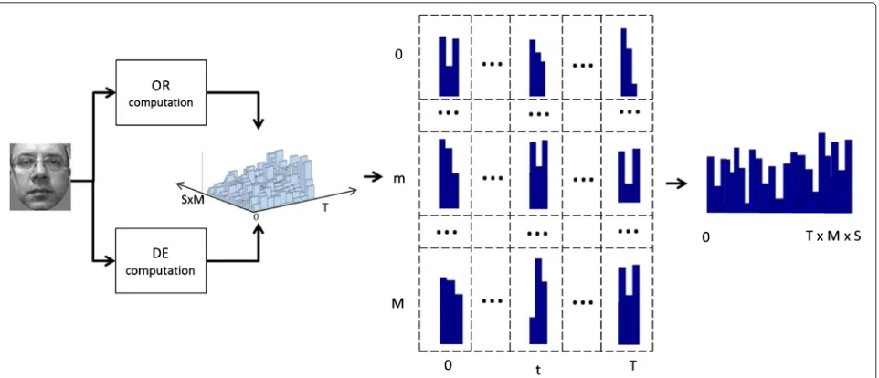
WLD [11] is a robust and powerful descriptor inspired to Weber’s law. It is based on the fact that the human per-ception of a pattern depends not only on the amount of change in intensity of the stimulus but also on the origi-nal stimulus intensity. The proposed descriptor consists of two components: differential excitation (DE) and gradient orientation (OR).
Differential excitation allows to detect the local salient pattern by means of a ratio between the relative intensity difference of the current pixel against its neighbors. The computational approach is similar to that used for LBP (a complete description is given in [11]). Moreover, the OR of the single pixel is considered.
When DE and OR are computed for each pixel in the image, we construct a 2-D histogram ofT columns and
M×S rows whereT is the number of orientations and
M×Sthe number of bins for the DE quantization with the meaning of [11]. Figure 6 shows how 2-D histogram is mixed in such a way to obtain a 1-D histogram that is more suitable for successive operations.
Furthermore, since for our purpose we had to account also for spatial information, we chose to use the SWLD approach [35] that, as for the spatial LBP, splits the image into sub-regions and computes an histogram for each of them. Finally, the histograms are concatenated in an ordered fashion.
3.3 Features subspace projection
The number of used features for face description highly affects both the computational complexity and the accuracy of classification. Indeed, a reduced number of features allows SVM to use easier functions and to per-form a better separation of clusters. In this work, LDA was considered to get a better data representation: this choice resulted from the high suitability experienced in traditional classification problems and in the preliminary experiments reported in [6].
3.3.1 LDA
LDA [12] is an alternative subprojection approach. In LDA, within-class and between-class scatters are used to formulate criteria for class separability. The optimizing criterion in LDA is the ratio of between-class scatter to the within-class scatter. The solution obtained by maxi-mizing this criterion defines the axes of the transformed space. Moreover, in LDA analysis, the number of non-zero generalized eigenvalues, and so the upper-bound in eigen-vectors numbers, isc−1 wherecrepresents the number of classes. Belhumeur at al. [12] demonstrated the robust-ness of this approach for face recognition and showed how LDA can sometimes be more discriminative. It is impor-tant to remark that the upper bound of eigenvectors for
Fig. 6WLD histogram construction process: the algorithm computes the DE and OR values for each pixel and constructs the 2-D histogram. The 2-D histogram is split into aM×Tmatrix, where each element is an histogram of S bins. Finally, the whole 1-D histogram is composed by the
concatenation of the previous matrix rows
LDA projection approach is a key factor also in terms of computational complexity that makes the workload of SVM lighter.
3.4 SVM classification
After data projection, in the proposed approach, gender, race, and age classifications were performed by using SVMs. In particular, three different SVM learning tasks were used: two-class support vector classification (SVC) for the gender problem; multi-class SVC for the race problem; and support vector regression (SVR) for the age estimation. All of these classification tasks can be biased by the data range (the j-th features of the data vector could take value in a different range with respect to the i-th one), and then, the opportunity of a scaling operation has to be analyzed in terms of classification performance. To analyze the scaling effect for soft biometric estimations, the following scaling approach was evaluated. Let xi,MAX and xi,MIN be the maximum and minimum values for the i-th features in the train-ing data (a list of labeled features data vector) and
yi,MAX,yi,MIN
the desired range after the scaling andNf the total number of features. The equation for the scale becomes
yi= (
xi−xi,MIN)·(yi,MAX−yi,MIN)
xi,MAX−xi,MIN +
yi,MIN (5)
wherexi is the initial value of thei-th feature andyi the scaled one. Finally, the scaling model is constructed by theNf pairs{xi,MAX,xi,MIN}and the pair{yi,MAX,yi,MIN}.
With regard to SVC, the C-support vector classi-fication (C-SVC) learning task implemented in the
well-known LIBSVM [90] was used. Given training vec-torsxi∈Rn,i=1,· · ·,l, in two classes, and a label vector y ∈ Rl such thatyi ∈ {1,−1},C-SVC [13, 14] solves the following primal optimization problem:
min w,b,ξ
1 2w
Tw+C l
i=1 ξi
subject to yi(wTφ(xi)+b)≥1−ξi, ξi ≥0,i=1,· · ·,l,
whereφ(xi)mapsxiinto a higher-dimensional space and C>0 is the regularization parameter. Due to the possible high dimensionality of the vector variablew, usually, the following dual problem is solved:
min α
1 2α
TQα−eTα
subject to yTα=0,
0≤αi≤C,i=1,· · ·,l,
where e =[1,· · ·, 1]T is the vector of all ones, Q is an
l×lpositive semidefinite matrix,Qij≡ yiyjK(xi,xj), and K(xi,xj) ≡ φ(xi)Tφ(xj)is the kernel function. After the dual problem is solved, the next step is to compute the optimalwas follows:
w= l
i=1
yiαiφ(xi) (6)
Finally, the decision function is
sgn(wTφ(x)+b)=sgn
⎛ ⎝l
i=1
Such an approach is suitable only for the two-class gender problems. For race classification, a multi-class approach was used, resorting to a “one-against-one” pro-cedure [91]. Letkbe the number of classes, thenk(k−1)/2 classifiers are constructed where each one trains data from two classes. The final estimation is returned by a voting system among all the classifiers. Many other methods are available for multi-class SVM classification; in [92], a detailed comparison is given with the conclusion that “one-against-one” is a competitive approach.
With regard to SVR, instead, the -SVR learning task was used. Given training points {(xi,zi),· · ·,(xl,zl)} where xi ∈ Rn is a features vector and zi ∈ R is the target output,-SVR [13, 14] solves the following primal optimization problem:
min w,b,ξ,ξ∗
1 2w
Tw+C l
i=1 ξi+C
l
i=1 ξi∗, subject to wTφ(xi)+b−zi≤+ξi,
zi−wTφ(xi)−b≤+ξi∗, ξi,ξi∗≥0,i=1,· · ·,l,
withC>0 and >0 as parameters. In this case, the dual problem is as follows:
min
α,α∗ 1 2
α−α∗TQ(α−α∗)+l
i=1
αi+αi∗
+
l
i=1
zi
αi−αi∗
subject to eT(α−α∗)=0,
0≤αi,αi∗≤C,i=1,· · ·,l,
and the approximate solution function for the dual prob-lem is as follows:
l
i=1
α∗−αK(x
i,x)+b
Finally, in the SVM, the output model is reported.
4 Experimental setup and results
In this section, the experimental evaluation of the frame-work devoted to soft biometric estimations is reported. In particular, the abovementioned biasing factors were evaluated on different data benchmarks incorporating also real-world contexts with challenging operating con-ditions.
Three different system settings were considered:
• the family of descriptors used to represent the facial features;
• the composition of the training set in terms of representatives of the classes to be predicted; • the scaling of the input variables in the features
vector to be supplied to the classifier.
Successively, the best configurations for training and scaling were tested over two real-world sources of bias:
• the spatial resolution of the facial image to be analyzed;
• the head pose of the subject in the scene.
To carry out the aforementioned analysis, two different experimental phases were performed. The first one was
carried out by using a large set of faces (more than 55,000) built by combining images available from different public datasets. The aim of this phase was to evaluate the perfor-mance of the soft biometrics estimation framework over images acquired under (quasi) ideal conditions (high reso-lution and frontal faces): in this way, the variability in clas-sification performance when using balanced/unbalanced training sets, different descriptors, and data projection strategies, with and without data scaling, can be accu-rately evaluated. In the second phase, images acquired in a real environment were used instead: in this way, boundary conditions were relaxed by introducing changes in head pose (i.e., non-perfectly frontal face) and vary-ing the distance from the camera (i.e., different spatial resolutions) with the aim to test the robustness of the different framework configurations under these two addi-tional real-world biases. Both experimental phases are detailed in the following subsections.
4.1 Experimental phase 1
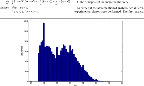
This experimental phase was carried out on two datasets built by properly merging two of the most representative publicly available repositories containing face images: the Morph [93] and Feret [94]. They consist of face images of people of different gender, race, and age, provided with complete annotation data. Moreover, both repositories present some replicated subject sampled in different dates (same person pictured in different years). The resolution of facial images is 200×240, 400×480, or 512×768 pixels. Starting from the available images, a first experimental dataset was built without taking into account the balanc-ing of the cardinality of each class. It consists of 46,669 male subjects and 9246 female subjects. The considered races were White, Black, Asian, and Hispanic with a cardinality respectively of 11,843, 41,334, 601, and 1889 subjects. Finally, the age distribution is represented in Fig. 7.
Moreover, two more balanced datasets were also built as subsets of the main one. The first one counts 8500 entries for each class of gender, whereas the second one is related to the race and counts 600 entries for each class (more balanced age group subsets cannot be built given the data distribution in the starting repositories).
The experimental results were obtained, on the afore-mentioned datasets, by means of an accurate cross val-idation procedure: the dataset under investigation was randomly split intokfolds (k = 5) and, for each of thek
validation steps,k−1 folds were used for training, whereas the remaining fold was used for evaluating the estima-tion/validation capabilities. Thekfolds were built using a strategy to retain, in each of them, the same ratio of ele-ments for the classes taken in the considered dataset: for example, in each fold, the ratio of male/female individu-als was kept about to 1:10. The class separation for the
gender estimation task was straightforward. On the other hand, for race estimation, facial images were split into four categories:White,Black,Asian, andHispanic. For the age issue, subjects were split into a number of categories equal to the number of the considered ages; the number of classes to be predicted was 42.
Face detection and normalization were then performed on each image of the selectedk-1 training folds and then the vectors of features were extracted, properly projected
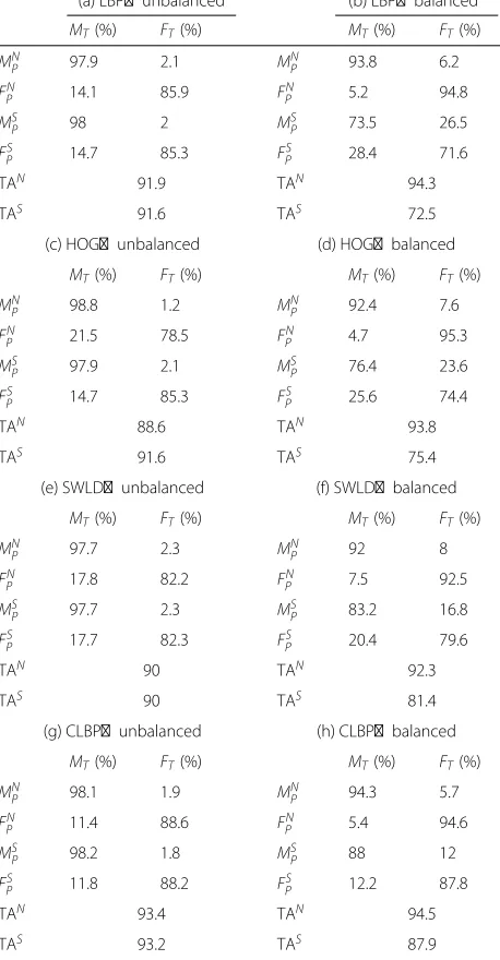
Table 1Gender confusion tables
(a) LBP—unbalanced (b) LBP—balanced
MT(%) FT(%) MT(%) FT(%)
MN
P 97.9 2.1 MNP 93.8 6.2
FN
P 14.1 85.9 FPN 5.2 94.8
MSP 98 2 MSP 73.5 26.5
FPS 14.7 85.3 FPS 28.4 71.6
TAN 91.9 TAN 94.3
TAS 91.6 TAS 72.5
(c) HOG—unbalanced (d) HOG—balanced
MT(%) FT(%) MT(%) FT(%)
MN
P 98.8 1.2 MNP 92.4 7.6
FN
P 21.5 78.5 FPN 4.7 95.3
MS
P 97.9 2.1 MSP 76.4 23.6
FS
P 14.7 85.3 FPS 25.6 74.4
TAN 88.6 TAN 93.8
TAS 91.6 TAS 75.4
(e) SWLD—unbalanced (f) SWLD—balanced
MT(%) FT(%) MT(%) FT(%)
MNP 97.7 2.3 MNP 92 8
FPN 17.8 82.2 FPN 7.5 92.5
MSP 97.7 2.3 MSP 83.2 16.8
FPS 17.7 82.3 FPS 20.4 79.6
TAN 90 TAN 92.3
TAS 90 TAS 81.4
(g) CLBP—unbalanced (h) CLBP—balanced
MT(%) FT(%) MT(%) FT(%)
MN
P 98.1 1.9 MNP 94.3 5.7
FN
P 11.4 88.6 FPN 5.4 94.6
MS
P 98.2 1.8 MSP 88 12
FS
P 11.8 88.2 FPS 12.2 87.8
TAN 93.4 TAN 94.5
TAS 93.2 TAS 87.9
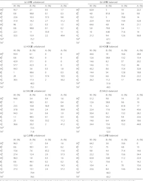
Table 2Race confusion tables
(a) LBP—unbalanced (b) LBP—balanced
WT(%) BT(%) AT(%) AT(%) WT(%) BT(%) AT(%) AT(%)
WN
P 95.7 2.1 0.5 1.7 WPN 62.8 5 10 22.2
BN
P 0.8 98.8 0.1 0.3 BNP 4.8 81.8 3.6 9.8
ANP 22.6 10.3 57.3 9.8 ANP 10.2 5 70.8 14
HN
P 31.9 14.2 2.7 51.2 HNP 22.4 10.4 14.4 52.8
WS
P 96 2.2 0.3 1.5 WPS 64.6 4.8 9.4 21.1
BSP 0.8 98.8 0.1 0.2 BSP 5.8 79.8 3.4 1.1
AS
P 22.1 11 55.9 11 ASP 10 4.40 71.6 14
HS
P 32.5 15.9 2.2 49.4 HSP 21.2 9.4 12.6 56.8
TAN 75.7 TAN 67.1
TAS 75 TAS 68.2
(c) HOG—unbalanced (d) HOG—balanced
WT(%) BT(%) AT(%) AT(%) WT(%) BT(%) AT(%) AT(%)
WN
P 93.9 6.1 0 0 WPN 44.6 10 16.6 28.8
BN
P 0.8 99.2 0 0 BNP 12.6 58.8 13.2 15.4
ANP 42.9 57.1 0 0 ANP 14.6 8.2 57 20.2
HN
P 57.7 42.3 0 0 HNP 14.6 13 15.2 46
WS
P 94.3 3.6 0.3 1.8 WPS 43.2 8.6 15.4 32.8
BSP 1 98.6 0 0.3 BSP 14.4 54 12.8 18.8
AS
P 20 12.1 57.4 10.5 ASP 15.8 6.6 55.4 22.2
HS
P 30.5 17.3 2 50.2 HSP 26.2 11.2 17 45.6
TAN 48.3 TAN 51.6
TAS 75.1 TAS 49.5
(e) SWLD—unbalanced (f) SWLD–balanced
WT(%) BT(%) AT(%) AT(%) WT(%) BT(%) AT(%) AT(%)
WNP 94.6 3.4 0.4 1.6 WPN 51.2 9.8 14 25
BN
P 1 98.5 0.1 0.4 BNP 12.6 58.8 9.6 19
AN
P 23.5 10.8 56.9 8.8 ANP 15 6.2 61.8 17
HNP 37.8 19.9 2.4 39.9 HNP 22.4 17.6 16.4 43.6
WS
P 94.3 3.4 0.4 1.9 WPS 50.4 8.2 13.2 28.2
BS
P 1.1 98.5 0.1 0.3 BSP 13.8 54.2 9.4 22.6
ASP 25 10.6 53.2 11.2 ASP 14.6 6.4 60.4 18.6
HSP 36.6 20.2 2 41.2 HSP 24.4 15.6 15.2 44.8
TAN 72.5 TAN 53.8
TAS 71.8 TAS 52.5
(g) CLBP—unbalanced (h) CLBP—balanced
WT(%) BT(%) AT(%) AT(%) WT(%) BT(%) AT(%) AT(%)
WNP 96.3 1.7 0.4 1.6 WPN 64.2 3.6 10.6 0
BN
P 0.6 99.1 0.1 0.2 BNP 7.2 75 4.8 13
AN
P 15.6 7.6 65.2 11.6 ANP 9.8 4.4 71.4 14.6
HNP 27.4 12.4 2.9 57.3 HNP 22.2 7.8 15.6 54.4
WS
P 96.3 1.8 0.3 1.6 WPS 62.8 3.60 11.2 22.4
BS
P 0.6 99.1 0.2 0.2 BSP 7.2 73.6 5 14.2
ASP 15.3 8.6 61.6 14.5 ASP 10.4 4 70 15.6
HS
P 27.3 13.1 2.4 57.2 HSP 22.6 8.4 14.6 54.4
TAN 79.4 TAN 66.3
TAS 78.5 TAS 65.2
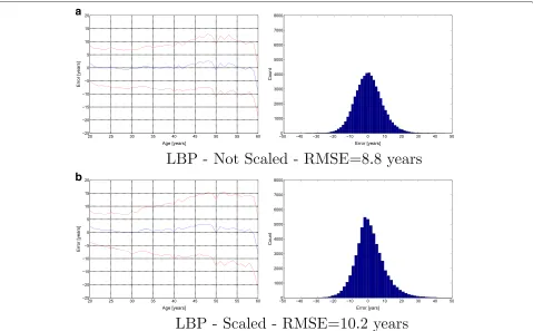
Fig. 8LBP ages mean error:left columnshows the mean age estimation error (blue line) and the standard deviation of age estimation error (red line). Right columnrepresents the empirical age estimation error distribution among all ages. (a) LBP—not scaled. (b) LBP—scaled
on the subspace defined by the LDA algorithm and finally supplied to the SVMs. After the training phase, the one-out fold was tested by using the available models. At the end of the iterative training/test process of the k fold method, the accuracy results were averaged.
The LBP algorithm1was spatially processed over a 5×5 grid, 8 neighbors, and 1 pixel radius; the CLBP algorithm was developed as reported in [9] and applied with the same parameters used for LBP. For the HOG operator, the VLFeat library2 was used with standard parameters as suggested in [10] leading to a feature vector of 2016 elements; the WLD operator was implemented following the work in [35] and setting T, M, and S, respectively, to 8, 4, and 4 over a 4 × 4 grid of the image having a final vector of features of 2048 elements. SVM (for gender and race classification and for age regression) was used as implemented in the LIBSVM library [90], and the radial basis function (RBF) kernel,K(x,y)=e−γx−y2, was used as suggested in [95] for non-linearly separable problems. Finally, the regularization parameterC was set to 1 and γ to 1/Nf where Nf is the number of features. In the case of scaling of the data in input to the SVM, the tar-get range was [0,1] for each variable in the LDA vector of features.
The results of the experimental phase 1 for gender and race are reported in Tables 1 and 2, respectively.
For the age estimation, that is a regression problem, the pairspredicted age/real ageof the whole k-fold procedure were considered and the average estimation error (blue line) and the standard deviations (red lines) are reported on the left side in Figs. 8, 9, 10, and 11. Let ibe a spe-cific age and Ni the corresponding number of entries; the age estimation error for thej-th entry of the ageiis defined as:
ei,j= ˆij−ij (8)
whereˆij is the predicted age andij is the age annotated in the dataset. Using the previous definition, it follows that the mean age estimation error for the age i can be defined as
ei= 1
Ni Ni
j=1
ei,j (9)
and the error variance as
σ2
i = 1
Ni Ni
j=1
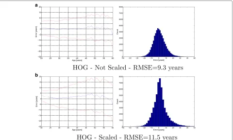
Fig. 9HOG ages mean error:left columnshows the mean age estimation error (blue line) and the standard deviation of age estimation error (red line). Right columnrepresents the empirical age estimation error distribution among all ages. (a) HOG—not scaled. (b) HOG—scaled
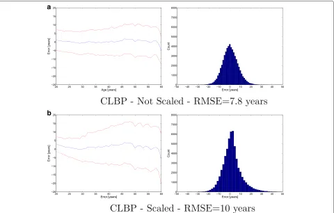
Fig. 11CLBP ages mean error:left columnshows the mean age estimation error (blue line) and the standard deviation of age estimation error (red line).Right columnrepresents the empirical age estimation error distribution among all ages. (a) CLBP—not scaled. (b) CLBP—scaled
Finally, for each age i, the RMS error (RMSEi) was computed as
RMSEi=
1
Ni Ni
j=1
(ei,j)2 (11)
and the total RMS error (RMSE) as
RMSE= 1
Na Na
j=1
RMSEj (12)
whereNais the number of ages between 20 and 60. The histograms of the whole age estimation errors over all ages and samples were constructed and plotted on the right side of Figs. 8, 9, 10, and 11.
Results for gender and race were considered in terms of confusion tables where the rows are referred to the pre-diction (subscript P) and the columns to the true class (subscript T). In detail, the first two rows represent the prediction for the non-scaled case (superscriptN), while the second two rows are referred to the scaled one (super-scriptS). The subtables (a), (c), (e), and (g) show the results for the unbalanced dataset; on the other hand, the subta-bles (b), (d), (f ), and (h) refer to the results of the balanced
subset. The total accuracy (TA) for both the scaled and non-scaled cases is reported in the last two rows of each subtable.
More specifically, Table 1 shows that, for gender estimation, the CLBP descriptor, using a balanced dataset and non-scaled values as input to the classifier, returned the best total classification accuracy (94.5 %). This trend was also confirmed if the average of correct estima-tions (taking into account all the possible combinaestima-tions of data scaling and dataset balancing) corresponding to each descriptor is considered. In fact, the CLBP classifi-cation rate was of 92.2 % which overcame the equivalent measurements obtained through the comparing descrip-tors (HOG 87.3 %, SWLD 88.4 %, and LBP 87.6 %).
account all the possible descriptors with no data scaling) of 93.7 % in the case of balanced dataset and 91.0 % in the case of unbalanced dataset.
To summarize, for gender estimation, the best configu-ration of the proposed framework can be assumed to use a CLBP classifier, learned on balanced dataset and working on non-scaled input data.
Race estimation problem is a very different problem due to the larger number of classes (four classes), the pres-ence of borderline cases, and the critical unbalancing of subjects among classes (there are just 600 Asian people against the 42,000 Black subjects).
Using the same evaluation criteria reported above, Table 2 shows that, forrace estimation, the CLBP descrip-tor, using an unbalanced dataset and non-scaled values as input to the classifier, returned the best total classification accuracy (79.4 %).
The average correct estimations (taking into account all the possible combinations of data scaling and dataset balancing) corresponding to each descriptor were LBP 71.5 %, HOG 56.1 %, SWLD 62.6 %, and CLBP 72.4 %.
Concerning the opportunity to scale in the range [0,1], the variables of the feature vectors and experi-ments evidenced that, taking into account all the possible
descriptors and combinations of dataset balancing, scaled data gave the best average correct estimations (67.0 %). However, an in-depth analysis of the confusion tables reveals as this result is mainly biased by the HOG descrip-tor, operating on the unbalanced dataset by means of non-scaled data, bad outcomes (48.3 %). With regard to all the other descriptors, the non-scaled data approach is not worse than the scaled one. Taking into account all the pos-sible descriptors, the unbalanced dataset for training led to a better average correct estimation both in the case of scaled data (75.1 % for unbalanced case and 58.8 % for bal-anced case) and non-scaled data (69.0 % for unbalbal-anced case and 59.7 % for balanced case).
The unbalanced dataset worked better because the number of Asiatic representatives is lower than the remaining classes, and therefore, in the case of the
balanced case, a low number of samples can be used for each class. In other words, if the number of repre-sentatives for each class of race is sufficiently large, the combination of CLBP, balanced dataset, and non-scaled input to the SVM seemed to be the best choice.
A compact view of the performance, for gender and race estimation, is presented in Fig. 12 by means of bar dia-grams. In particular, Fig. 12a refers to gender estimation, whereas Fig. 12b refers to race estimation.
Finally, the age estimation was addressed as a regres-sion problem and, in this case, having 42 classes to be predicted, the balanced dataset was not built (since there were not enough representatives in each class). The exper-imental results, reported in Figs. 8, 9, 10, and 11, demon-strated that the CLBP without data scaling was the best performing descriptor (RMSE = 7.8 years). The best
average correct estimation (taking into account both com-binations of data scaling/not scaling) was again obtained with CLBP (RMSE=8.9 years) which overcame the other descriptors (LBP-RMSE=9.5 years; HOG-RMSE=10.4
years; SWLD-RMSE = 10.4 years). Concerning the
opportunity to scale the data, experimental results demonstrated that non-scaled data led to a better aver-age regression accuracy (RMSE=8.7 years) with respect to the case in which data fed into SVR were scaled in the range [0,1] (RMSE = 10.9 years). It is interesting to observe that the error distribution in the age estimation problem (see plots on the right of Figs. 8, 9, 10, and 11) revealed a Gaussian trend (around the zero value) with a steep decrease, demonstrating that in the most of age classification cases, the estimations were quite correct.
4.2 Experimental phase 2
In this phase, experiments were carried out on facial images acquired in a real environment: in this way, boundary conditions were relaxed with respect to pre-vious experimental phase. In particular, changes in head pose (i.e., non-perfectly frontal face) and distance from the camera (i.e., different spatial resolutions) were also considered as factors of classification/regression bias. A dataset of seven subjects (five males and two females, all belonging to the white race and age ranging from 23 to 48 years) was built on purpose with 900 images per sub-ject: in 300 images, subjects were at a distance of 75 cm from the camera and they assumed a close frontal pose (this subset of images were labelled as IFC, where the subscript stands for frontal-close); in other 300 images, subjects were at a distance of 75 cm from the camera but they performed a head rotation in the range [10°, 30°] (this subset of images was labelled asIRC, where the sub-script stands for rotated-close). Finally, in the remaining 300 images, subjects were at a distance of 165 cm from the camera and they assume a close frontal pose (this subset of images were labelled asIFF, where the subscript stands for frontal-far). In the case where the subjects were closer to the camera, the resolution of the facial patch is about [240× 180] pixels, whereas in the case where the sub-jects were farther from the camera, their facial patch is of about [100 ×70] pixels. Some examples of the three aforementioned subsets of images are reported in Fig. 13 where columns 1–3 report frontal-close images, columns
Table 3Gender estimation performance for the lab dataset
LBP (%) HOG (%) SWLD (%) CLBP (%)
IFC 98.4 97.9 98.4 98.6
IRC 95.7 85.3 92.1 97.9
IFF 88.4 97.5 87.9 89.0
IFCis referred to the frontal-close images,IRCto the rotated-close images, andIFFto the frontal-far images
Table 4Race estimation performance rate for the lab dataset
LBP (%) HOG (%) SWLD (%) CLBP (%)
IFC 97.7 93.3 89.2 96.1
IRC 97.5 86.0 84.6 93.2
IFF 97.1 92.4 89.9 89.1
IFCis referred to the frontal-close images,IRCto the rotated-close images, andIFFto the frontal-far images
4–6 report rotated-close images, and columns 7–9 report frontal-far images.
Experiments were carried out as follows: the facial datasets built in the experimental phase 1 was used to set the projection (through LDA), classification/regression (through SVM), and scaling models. These models were then stored and exploited, without any intervention, dur-ing all the soft biometric estimations carried out in the experimental phase 2.
In this case, due to the dataset composition, the mea-surement of the error for age prediciton was slightly modified as follows: letNs the numbers of subjects and Nf the numbers of frames for each subject (given a pose configuration).
The age estimation was treated with an RMS age esti-mation error.
RMSEj= 1 Nf Nf
i=1
ˆ θi,j−θj
2
(13)
whereθˆi,jis the age estimation for thei-th frame of thej-th subject andθjis the real age of thej-th subject. The mean RMS error (for all the subjects) is defined as
RMSE= 1
Ns Ns
j=1
RMSEj (14)
Finally, letei,j =
ˆ θi,j−θj
be the age estimation error for thei-th frame of thej-th subject andejits mean among theNf frames. The error variance of thej-th subject is as follows:
Table 5Age estimation RMSE for the lab dataset
LBP HOG SWLD CLBP
IFCRMSE 7.7 14.2 9.5 7.6
IRCRMSE 8.3 16.6 9.5 7.9
IFFRMSE 9.2 14.6 10.6 9.4
IFCσ2 12.2 15.9 19.3 12.9
IRCσ2 15.8 31.8 31.6 17.8
IFFσ2 9.1 21.5 26.7 14.9
σ2
j = 1
Nf Nf
i=1
(ei,j−ej)2 (15)
and the total mean variance is defined as
σ2= 1
Ns Ns
j=1 σ2
j (16)
The experimental outcomes of this phase are reported in Tables 3, 4, and 5 and Figs. 14 and 15. In particular, tables report gender, race, and age estimation correctness
for all the descriptors and over all the three experimental conditions (frontal-close imagesIFC, rotated-close images
IRC, frontal-far images IFF). It is very important to highlight here that the best configurations (revealed by experimental phase 1) for balancing and scaling strategies were used and that, due to the lack of statistical signifi-cance (i.e., few subjects), the aim of the test onIFCimages was not to evaluate the robustness of the framework (as largely tested in the previous subsection) but to have a reference point in the evaluation of the influence of pose and resolution. From this point of view, tables have to
Fig. 15Age RMSE (a) and variance (b) for lab dataset: each group of columns is referred to (fromleft to right) the frontal-close images (IFC), the rotated-close images (IRC), and the frontal-far images (IFF) configuration
be exploited to understand how much the performance of the various configurations of descriptor, dataset bal-ancing, and scaling strategies are influenced by pose and resolution changes. From the results, it is evident that the descriptor that is less sensitive to the image resolution is HOG (where a decrease of 0.4 % for gender, 0.9 % for race, and 0.4 years for age can be observed) and this is due to the fact that it is edge based (able to capture coarse texture information, as opposed to the other investigated meth-ods able to represent finer structures). Unfortunately, the HOG descriptor experienced the maximum decrease in
performance in the case of changes in pose (12.6 % for gender, 7.3 % for race, and 2.4 years for age) where the most robust behavior was obtained by the CLBP (0.7 % for gender, 2.9 % for race, and 0.3 years for age) which, by using a more sophisticated encoding strategy, was able to handle variations in facial patterns.
5 Conclusions
been presented. Firstly, different facial descriptors (LBP, HOG, SWLD, CLBP), training datasets, and data scal-ing approaches have been extensively tested in a recently introduced common framework including a data reduc-tion step (making use of linear discriminant analysis) and a final SVM classification step. Successively, robust-ness in unconstrained scenario, with scaling and rotation of the target with respect to the acquisition device, has been studied. Experimental evaluations have been carried out on benchmark data built from both publicly avail-able datasets and from image sequences acquired in lab environment. Results highlighted that the best average performances have been reached by the CLBP operator in all the estimation problems. This work proved that the non-scaled features vector approach is preferable to the scaled one and that balanced class cardinalities dur-ing dataset builddur-ing can give better performances. More-over, tests have been performed over the lab dataset with relaxed boundary conditions which proved that the CLBP operator outperforms the other descriptors in terms of average estimation performance in the presence of scaling and rotation. Future works will aim at extending the lab dataset both in terms of number of subjects and pose and resolution variability, in order to have more significative statistics.
Endnotes
1The on-line implementation, available at http://www.
bytefish.de. was used. 2http://www.vlfeat.org.
Competing interests
The authors declare that they have no competing interests.
Acknowledgements
This work has been supported in part by the “2007–2013 NOP for Research and Competitiveness for the Convergence Regions (Calabria, Campania, Puglia and Sicilia)” SARACEN with code PON04a3_00201 and in part by the PON Baitah, with code PON01_980.
Received: 31 October 2014 Accepted: 20 October 2015
References
1. T Martiriggiano, M Leo, T D’Orazio, A Distante, inInnovations in Applied Artificial Intelligence.Lecture Notes in Computer Science, ed. by M Ali, F Esposito. Face recognition by kernel independent component analysis, vol. 3533 (Springer, Berlin Heidelberg, 2005), pp. 55–58
2. AK Jain, SC Dass, K Nandakumar, inBiometric Authentication. Soft biometric traits for personal recognition systems (Springer, Berlin Heidelberg, 2004), pp. 731–738
3. P Carcagnì, D Cazzato, M Del Coco, C Distante, M Leo, inComputer Vision-ECCV 2014 Workshops. Visual interaction including biometrics information for a socially assistive robotic platform (Springer International Publishing, Gewerbestrasse 11 CH-6330 Cham (ZG)Switzerland, 2014), pp. 391–406 4. A Tapus, C Tapus, MJ Mataric, inIEEE International Conference on
Rehabilitation Robotics (ICORR). The use of socially assistive robots in the design of intelligent cognitive therapies for people with dementia (IEEE Computer Society, 10662 Los Vaqueros Circle, Los Alamitos, California, 2009), pp. 924–929
5. R Bemelmans, GJ Gelderblom, P Jonker, L De Witte, Socially assistive robots in elderly care: a systematic review into effects and effectiveness. J. Am. Med. Dir. Assoc.13(2), 114–120 (2012)
6. Carcagnì, M Del Coco, P Mazzeo, A Testa, C Distante, inVideo Analytics for Audience Measurement.Lecture Notes in Computer Science. Features descriptors for demographic estimation: a comparative study (Springer, International Publishing, Gewerbestrasse 11 CH-6330 Cham
(ZG)Switzerland, 2014), pp. 66–85
7. T Ojala, M PietikÀinen, D Harwood, A comparative study of texture measures with classification based on featured distributions. Pattern Recognit.29(1), 51–59 (1996)
8. T Ojala, M Pietikainen, T Maenpaa, Multiresolution gray-scale and rotation invariant texture classification with local binary patterns. Pattern Anal. Mach. Intell. IEEE Trans.24(7), 971–987 (2002)
9. F Ahmed, E Hossain, ASMH Bari, A Shihavuddin, inComputational Intelligence and Informatics (CINTI), 2011 IEEE 12th International Symposium On. Compound local binary pattern (CLBP) for robust facial expression recognition (IEEE Computer Society, 10662 Los Vaqueros Circle, Los Alamitos, California, 2011), pp. 391–395
10. N Dalal, B Triggs, inIEEE Computer Society Conference on Computer Vision and Pattern Recognition (CVPR). Histograms of oriented gradients for human detection, vol. 1 (IEEE Computer Society, 10662 Los Vaqueros Circle, Los Alamitos, California, 2005), pp. 886–893
11. J Chen, S Shan, C He, G Zhao, M Pietikainen, X Chen, W Gao, WLD: a robust local image descriptor. IEEE Trans. Pattern Anal. Mach. Intell.32(9), 1705–1720 (2010)
12. PN Belhumeur, JP Hespanha, D Kriegman, Eigenfaces vs. fisherfaces: recognition using class specific linear projection. IEEE Trans. Pattern Anal. Mach. Intell.19(7), 711–720 (1997)
13. C Cortes, V Vapnik, Support-vector networks. Mach. Learn.20(3), 273–297 (1995)
14. BE Boser, IM Guyon, VN Vapnik, inProceedings of the Fifth Annual Workshop on Computational Learning Theory.COLT ’92. A training algorithm for optimal margin classifiers (ACM, New York, NY, USA, 1992), pp. 144–152 15. Z Sun, G Bebis, X Yuan, SJ Louis, inIEEE Workshop on Applications of
Computer Vision. Genetic feature subset selection for gender classification: a comparison study (IEEE Computer Society, 10662 Los Vaqueros Circle, Los Alamitos, California, 2002), pp. 165–170
16. N Sun, W Zheng, C Sun, C Zou, L Zhao, ed. by J Wang, Z Yi, J Zurada, B-L Lu, and H Yin. Advances in Neural Networks - ISNN.Lecture Notes in Computer Science, vol. 3972 (Springer, Berlin Heidelberg, 2006), pp. 194–201 17. E Mäkinen, R Raisamo, An experimental comparison of gender
classification methods. Pattern Recognit. Lett.29(10), 1544–1556 (2008) 18. M Sakarkaya, F Yanbol, Z Kurt, inIEEE 16th International Conference on
Intelligent Engineering Systems (INES). Comparison of several classification algorithms for gender recognition from face images (IEEE Computer Society, 10662 Los Vaqueros Circle, Los Alamitos, California, 2012), pp. 97–101
19. C Ng, Y Tay, B-M Goi, inPRICAI 2012: Trends in Artificial Intelligence.Lecture Notes in Computer Science, ed. by P Anthony, M Ishizuka, and D Lukose. Recognizing human gender in computer vision: a survey, vol. 7458 (Springer, Berlin Heidelberg, 2012), pp. 335–346
20. R Brunelli, T Poggio, Face recognition: features versus templates. IEEE Trans. Pattern Anal. Mach. Intell.15(10), 1042–1052 (1993)
21. J-M Fellous, Gender discrimination and prediction on the basis of facial metric information. Vis. Res.37(14), 1961–1973 (1997)
22. S Mozaffari, H Behravan, R Akbari, in20th International Conference on Pattern Recognition (ICPR). Gender classification using single frontal image per person: combination of appearance and geometric based features (IEEE Computer Society, 10662 Los Vaqueros Circle, Los Alamitos, California, 2010), pp. 1192–1195
23. H Abdi, D Valentin, B Edelman, AJ O’Toole, More about the difference between men and women: evidence from linear neural networks and the principal-component approach.24, 539 (Pion Ltd, 1995)
24. S Tamura, H Kawai, H Mitsumoto, Male/female identification from 8×6 very low resolution face images by neural network. Pattern Recognit.
29(2), 331–335 (1996)