Icing Forecasting of High Voltage Transmission Line Using Weighted Least Square Support Vector Machine with Fireworks Algorithm for Feature Selection

Article

Icing Forecasting of High Voltage Transmission Line

Using Weighted Least Square Support Vector

Machine with Fireworks Algorithm for Feature

Selection

Tiannan Ma *,† and Dongxiao Niu †

Departemnt of Economics and Management, North China Electric Power University, Beijing 102206,China; [email protected]

* Correspondence: [email protected] or [email protected]; Tel.: +86-185-1562-1058 † _{These authors contributed equally to this work.}

Abstract: Accurate forecasting of icing thickness has a great significance for ensuring the security and stability of power grid. In order to improve the forecasting accuracy, this paper proposes an icing forecasting system based on fireworks algorithm and weighted least square support vector machine (W-LSSVM). The method of fireworks algorithm is employed to select the proper input features with the purpose of eliminating the redundant influence. In addition, the aim of W-LSSVM model is to train and test the historical data-set with the selected features. The capability of this proposed icing forecasting model and framework is tested through the simulation experiments using real-world icing data from monitoring center of key laboratory of anti-ice disaster, Hunan, South China. The results show that the proposed W-LSSVM-FA method has a higher prediction accuracy and it may be a promising alternative for icing thickness forecasting.

Keywords: icing forecasting; fireworks algorithm; least square support vector machine; feature selection

1. Introduction

In recent years, the icing disaster caused by the global extreme weather has brought great damage to the transmission lines and equipment in most parts of China. For example, in 2008, a large area of freeze damage occurred in the south of China, and the power grid of several provinces suffered serious damage which brought particularly serious economic losses to the power grid corporation. The research on the icing prediction of transmission lines is able to help us to develop effective anti-icing strategies, which can ensure the safe and reliable operation of transmission lines, so as to ensure the sustainable development of the power grid construction. Taking into account the influence of meteorological factors such as temperature, wind speed, wind direction, humidity and so on, the transmission line icing prediction can be determined by establishing the nonlinear relationship between the icing thickness and its influencing factors. The accuracy of icing prediction directly affects the quality of the prediction work.

regression model may cause the loss of important influence factors information, thus reducing the accuracy of icing prediction. Therefore, intelligent forecasting models are hot research topics in the present study, which are based on the combination of modern computer techniques and mathematics.

Some researchers have considered related factors such as temperature, humidity, wind speed in icing forecasting intelligent models and also applied the BP neural network as the icing forecasting model. For example, the paper[4][7][9] respectively use the single BP model to verify its effectiveness and feasibility in icing forecasting, the experiment results show that BP neural network has the ability to establish the nonlinear relationship between the factors and the icing thickness. However, the single BP model is usually easy to fall into local optimum and cannot reach the expected accuracy in icing forecasting. Therefore, some researchers attempt to improve the BP neural network to build the icing forecasting model. For example, paper [12] proposes a Takagi-Sugeno fuzzy neural network to predict the icing thickness under the extreme freezing weather conditions. And paper [8] utilizes the genetic algorithm (GA) to optimize the BP neural network to improve the convergence ability. Although the improved BP neural network could improve the prediction accuracy, it still shows the shortcomings of poor learning ability and performance.

In order to improve the forecasting accuracy and strengthen the learning ability, some scholars start to adopt the support vector machine (SVM), which has a more powerful nonlinear processing ability and high-dimensional mapping capability, to build the forecasting model of icing thickness. Paper [3] and [15] utilizes some factors (such as temperature, humidity, wind speed etc.) as the input and the icing load is the output of prediction model based on support vector machine; the simulation results show this model is available in the icing forecasting. And in paper [14], the least squares support vector machine (LSSVM) is adopted to build the icing prediction model and the case study shows the effectiveness and correctness of the proposed method. The single SVM model has the advantages of repeated training and faster convergence speed and so on. However, due to the influence of the control parameters, the single SVM model is difficult to achieve the expected precision. Based on the defects of single SVM, some people propose the combination algorithm to pursue the higher accuracy of icing forecasting. Paper [5] presents two different forecasting systems that are obtained by using support vector machines whose parameters are also optimized by genetic algorithm (GA). Paper [13] proposes a combination icing thickness forecasting model based on particle swarm algorithm and SVM. And paper [1] proposes a brand new hybrid method which is based on weighted support vector machine regression (WSVR) model to forecast the icing thickness and particle swarm and ant colony (PSO-ACO) to optimize the parameters of WSVR. In combination models, the optimal parameters of SVM can be obtained by optimizing calculation with optimization algorithm, which could ensure higher prediction precision. However, only few researches have adequately considered the relationship between factors and icing thickness, most of the researches only put the fundamental meteorological factors (temperature, humidity, wind speed) into the established methods. In this way, those stream of methods may fail to consider various influential factors of icing forecasting.

Therefore, some researchers start to consider more impact factors and apply other methods to study the icing forecasting problem. Paper [2] proposes an ice accretion forecasting system (IAFS) which is based on a state-of-the-art, mesoscale, numerical weather prediction model, a precipitation type classifier, and an ice accretion model. Paper [6] studies the medium and long term icing thickness forecasting on the transmission lines and presents a forecasting model based on the fuzzy Markov chain prediction; Paper [10] studies the icing thickness forecasting model by using fuzzy logic theory. Paper [11] establishes a forecasting model which is based on wavelet neural networks (WNN) and continuous ant colony algorithm (CACA) to predict the icing thickness. However, it has been often noticed in practice that increasing the factors to be considered in a model may degrade its performance, if the number of factors that are used to design the forecasting model is small relative to the icing thickness. Thus the feature selection is important when faced with the problem of obtaining more useful influential factors in icing forecasting task.

colony optimization algorithm [21] and so on. Those algorithms have shown their performance in feature selection problem because they can find the optimal minimal subset at each iteration time. Additionally, it can be seen that the swarm intelligent algorithms are easy to be realized by computer programs compared with the mathematical programming approaches. Support vector machine(SVM), proposed by Vapnik, is based on the statistic theory, and has been widely applied into the forecasting system, however, SVM is complex and difficult to calculate. For solving the emerged problem of SVM, least square support vector machine (LSSVM) has been proposed to solve the complicated quadratic programming problem. To some extent, LSSVM is an extension of SVM, and it projects the input vectors into the high-dimensional space and constructs the optimal decision surface, then turns the inequality computation of SVM into the equations calculation through the risk minimization principle; thus, reducing the complexity of calculation and accelerating the operation speed.

Through the above analysis, a new idea which can improve the accuracy of icing forecasting is presented. A new model of using weighted least square support vector machine and fireworks algorithm is established for icing forecasting. The information redundancy and the influence of the noise on the accuracy of ice forecasting can be reduced through the feature selection, so as to provide the appropriate input vector for the W-LSSVM model. By weighting the LSSVM, it can improve the generalization ability and nonlinear mapping ability of the algorithm, which can guarantee the higher fitting accuracy in training and learning. The rest of the paper is organized as follows. In Section 2, we will discuss the basic theory of fireworks algorithm (FA) and its application in feature selection. In Section3, we will introduce the weighted least square support vector regression model. A case study is demonstrated through the computation and analysis in Section 4. Finally, the conclusions are presented in Section 5.

2. Fireworks algorithm for feature selection

The fireworks algorithm, first proposed by Tan, is a brand new global optimization algorithm. In the fireworks algorithm, each fireworks can be considered as a feasible solution of the optimal solution space, the process of fireworks explosion can be regarded as the process of searching the optimal solution.

A fireworks algorithm can be generally applied to any combination optimization problem as far as it is possible to define:

(1) In the feasible solution space, a certain number of fireworks are randomly generated, each of which represents a feasible solution(subset).

(2) According to the objective function, calculate the fitness value fitness(x_i)of each fireworks to determine the quality of fireworks, in order to produce a different number of sparks Siunder different explosive radiusRi. Judging from the fitness value, the fitness value is better, the more sparks can be produced in the smaller areas; in the contrary, the fitness value is worse, the less sparks can be produced in the larger areas.





 

 



 _N

i

i i i

x f y

x f y M S

1 max max

)) ( (

) (





(1)

 









 

  

 _N

i i i i

y x f

y x f R R

1

min min

) ( ˆ





(2)

Whereymax,yminrepresent the maximum and minimum fitness value respectively in the current

population; f

 

xi is the fitness value for fireworksxi; M is a constant, which is used to adjust the

number of the explosive sparks; Rˆ is a constant to adjust the size of the fireworks explosion radius;



_{is machine minimum, which is used to avoid zero operation.}

(3) Produce explosive sparks. In the fireworks algorithm, when the new fireworks

x

jare





k

z

U

R

x

x

ˆ

_ik



_ik



_i





1

,

1

,

1





(3)

Where

R

iis the explosive radius; U(1,1)represents the random number obeying the uniform

distribution in the range

[



1

,

1

]

.

(4) Produce variant sparks. The production of the variant sparks is to increase the diversity of the explosive sparks. The variant sparks of the fireworks algorithm is to mutate the explosive sparks by the Gauss mutation, which will produce the Gauss variation sparks. Suppose that the fireworksxiwere selected to carry out the Gauss variation, then thekdimension Gauss variation is

used as follows:

x

ˆ

ik



x

ik



e

, in whichxˆikis the kdimensional variation fireworks, anderepresents

obeying the Gauss distribution ofN(1,1).

Explosive sparks and mutation sparks respectively generated by the explosive and mutation operators in the fireworks algorithm may exceed the boundary of the feasible regionΩ. Therefore they need to be mapped to new positions by mapping rules, and the formula is as follows:



UBk LBk



ik k LB

ik

x

x

x

x

x

ˆ



_,



ˆ

%

_,



_, (4)

Where

x

UB,kand

x

LB,kare the upper and lower bounds of the solution space in the dimension k.

(5) Select the next generation fireworks for iterative calculation. In order to transmit the information of excellent individuals to the next generation, it is needed to select a certain number of individuals from the explosive sparks and mutation sparks as the next generation of fireworks. Suppose the number of candidates isKand the population quantity isN , the individual with the optimal fitness value will be determined to be the next generation of fireworks. For the rest

N



1

fireworks, select them by the probability calculation. For the fireworksxi, the probability

calculation formula of being selected is:







K x

j i i

j

x x R x

p( ) ( )

(5)









 

   

K x

j i K

x

j i i

j j

x x x

x d x

R( )

(6)

In the above formula,

R

(

x

)

is the sum of the distances between the individuals in the current candidate set. In the candidate set, if the individual density is relatively high, namely there are other candidates around the individual, the probability of the individual being selected will be reduced.

(6) Judge the ending condition. If the ending condition is satisfied, jump out of the program and output the optimal results; if not, return to the step (2) and continue to circulate.

The main purpose of feature selection is to find a subset from specific problem, which can be described to find the combination optimization problem of fireworks algorithm. It is very necessary to select the appropriate fitness function in the combination optimization problem, therefore, this paper will consider the forecasting accuracy and number of selected features as the main factors in the fitness function, which is shown as follows:

 

 

]

) ( 1 [

i i

i

x Numfeature b

x r a x

fitness     ₍₇₎

Where

r

 

x

i represents the forecasting accuracy of particle

x

i;Numfeature(xi)is the number of selected features;

a

,

b

is the constant between 0 and 1. Here, if a particle obtain a higher accuracy and lesser number of features, then fitness value will be better.

In the fireworks algorithm, each fireworks represents a feature subset. Letxj 

 

0,1,j1,2,,n,where

j

is the

jth

feature, when xj 0, this means the

jth

feature isn’t selected; otherwise, when

x

j



1

, the

jth

feature is selected. However, before use FA to select the



















 



 

 



N

i

k k i N

i

j j i N

i

k k i j j i

jk

x x x

x

x x x x Cor

1

2 1

2 1

) (

(8)

WhereCorjkis the correlation coefficient between vectorjand vectork;

j i

x

represents theith factor of vectorj_;xj_{is the average value of vector j;} k

i

x

represents theith factor of vectork;_xk_{is the}

average value of vectork.

In the icing prediction, the rule of determining the feature subset is as follows: Calculate the correlation coefficients between each influencing factor and the icing thickness according to the formula (8), and sort them in the order from big to small. Set the number of all of the feature sets isc , the characteristics of the correlation coefficientCor are set into a subset, the rest characteristics are randomly distributed into otherc1subsets, and all the

c

feature sets are put into the setSi,i1,2,,c.Calculate the fitness function value fitness(Si),i1,2,,cof each feature set

according to the above FA algorithm steps. Judge whether any subset is satisfied with the ending condition (an expected forecasting accuracy



). If there exists, output the result. If not, select the feature of the highest correlation coefficient from the subset with the maximum fitness and the next subset, and put it into the current set, and then enter a new iteration(Note: the same feature are not allowed in the same subset). The rule is shown in Fig.1.

Figure.1 The rule of forming new feature subset

As shown above, assuming the set of existing subsets is S_i,i1,2,3,4, all the subsets are substituted into the model using the FA algorithm to calculate the fitness function fitness(i),i1,2,3,4corresponding to each subset, and sort them in the descending order:

) 4 ( )

3 ( )

2 ( )

1

( fitness fitness fitness

fitness   

If all the subsets are not up to the expected condition, select the feature of the highest correlation coefficient and put it into the Subset 1 to form the New Subset 1. Then, select the feature of the highest correlation coefficient from the Subset 1 with the maximum fitness and the next Subset 3, and put it into the Subset 2 to form the Subset 3, and then repeat the steps until the last group of New Subset 4 is finished. Finally, all the new subsets are put into the next iteration until the expected condition is satisfied, and then output the result.

3 Weighted least square support vector regression model

3.1 Basic theory of LSSVM

LSSVM is an extension of support vector machine. It transfers the input vector into high dimensional space through nonlinear casting and constructs the optimal decision surface, and then turns the arithmetic of SVM inequalities into equations calculation according to the risk minimization principle.

output, and

N

is total number of sample. The regression model of the sample is:

 

x

 

x

b

y



T







w

(9)

Where



(



)

represents casting the training data to a high dimensional space; w_{is the weighted}

vector; bis the bias.

For LSSVM, the optimization problem can be transformed into:







N 1 i i

γ

min

w

T

w

ξ

2

2

1

2

1

(10) t

s _yi T

 

_xi b_ξi,i1,2,3,_N;

w



(11)

Where



is the punishment coefficient for balancing the complexity and accuracy;



i is the

estimated error. To solve the above equations, it must be transferred to the Lagrange function and that will be solved in Section 3.3.

3.2 Improvement of LSSVM

(1) Horizontal weighted input vectors

The mode of multi-inputs and single output is always emerged in icing forecasting task. The value of the input vectorxiis distributed along with the time and the influence of the actual value of

the icing thickness at different times can be reflected by the weighted processing. Therefore, the input vector can be weighted according to the following formula:





k l

x

xˆi  ki 1 n i, 1,2,,







(12)

Where xˆiis the weighted vector; xkiis the original vector; kis the dimension number of input

vectors;



is a constant.

(2) Vertical weighted training data set

The predicted value of the ice forecasting is not only related to the elements in the input vector, but also with the sample group. This correlation is reflected as: near distance samples have a great influence on the prediction, but the distant samples have little effect on the forecasting. So it is necessary to reduce the impact of near distance samples on the prediction model by using different membership values of the current icing thickness. The membership values can be calculated by using linear membership



i, and the equation is as follows:

1 0 , / ) 1 (      i

i  i  N 

 (13)

Where



iis the value of membership;



is a constant between 0 and 1;

i



1

,

2

,



,

N

. The input

sample set can be transformed into:



 









x y x y xN yN N



T 1, 1,1 2, 2,2  , , (14) The determination value of



directly impacts the performance of LSSVM, thus the value of



can be obtained by calculating the gray correlation coefficient. The gray correlation coefficient is calculated as follows:





(max) (max) (min) ) ( ), ( 0 ki ki ki ki i k x k x r          (15) ] 1 , 0 [ ) ( ) (

0  



_ki x k x_i k  ₍₁₆₎







  N k i i r x k x k

1

0( ), ( )

Considering the multi-inputs and single output of icing forecasting, this paper will letx0 Y,Y



y1,y2,,yN



.

3.3 Weighted LSSVM

Apply the improvements of Section 3.2 into LSSVM to form a weighted LSSVM, thus the objective function can be described as follows:



  N 1 i i i γ

min wTw ξ2

2 1 2 1 _ (18) t

s _yi T

 

_xi b_ξi,i1,2,3,_N;

w



(19)

In order to solve the above problem, the Lagrange function is established:







 

i i



T N

i N

T

i b y

i

i i

γ α

b

L    

    

 w w ξ w ξ

ξ

w i i i

2 x 1 1 2 1 2 1 , ,

,    ₍₂₀₎

Where



i is Lagrange multiplier. Each variable of the function is derivated, and is made to zero:

 

                                       0 0 0 0 0 0 1 1 yi i b α L i γ αi L αi b L xi αi L T i N i N i ξ w ξ ξ w w   (21)

Eliminatewandξ i,and transform it into the following problem:

                        y a b I n T n 0 0 1 1  Ω e e (22)

Where

   

_xi _xi

T







Ω ,

e

n





1

,

1

,...,

1



T,

α





α

1

,

α

2

,...,

α

n



,y



y1,y2,...,yn



T



Solve the above equations and obtain the following equation：

 

x α K





b

y N 1 i i   

 xi,x (23)

Where

K



x

i

,

x



is the kernel function. This paper uses the wavelet kernel function



         N i i i i i x x x x K 1 ) , ( 

 _in y

 

x :

 

x x x b

y N i N i i i i i     

1



_1

) (

 

 (24)

) 2 exp( ) 75 . 1 cos( ) ( 2 x x

x   

 (25)

Finally, the regression equation of W-LSSVM is obtained as:

 

x x x x x b

y N i N i i i i i i i         

1



_1

2 ]} 2 ) ( exp[ ] ) ( 75 . 1 {cos[ 

 (26)

4 Experiment simulation and results analysis

The process of using FA for feature selection and W-LSSVM for icing forecasting is shown in

Fig.2. As we can see, the proposed icing forecasting system mainly includes three parts: FA based feature selection (Part 1), W-LSSVM based icing forecasting (Part 2) and W-LSSVM based retraining

and testing (Part 3). If the established feature subset of each fireworks cannot reach the required

value, it will return the process and continue to build the feature subset until finding the best feature subset. So in the proposed icing forecasting system, the purpose of Part 1 is to make the iterative

optimization and count the number of selected features of each fireworks; and the aim of Part 2 is to calculate the accuracy of each fireworks; then we can obtain the fitness value of each fireworks

through calculating the formula (7). Finally, we will retrain the W-LSSVM and evaluate the testing set by adopting the best subset in Part 3.

Initialize the feature subsets

Initialize the population and related parameters

Calculate fitness calculate explosive radius and

sparks number

Update the individual coordinates one by one

Select next generation fireworks for iterative calculation by using probability

pl

Stop criteria Generate new

subsets

No

Get optimal feature subset

Yes

Original data

Horizontal weighted input vectors

Data pretreatment

Training set Testing set

Training with selected features

Training with selected features

Calculate the forecasting accuracy Give the feature

subset

Retrain the WLSSVM based icing forecasting with selected

features

Test the WLSSVM with testing set

Evaluate the forecasting results with RE, MAPE,MSE

Part 1 Part 2

Part 3

Use the new generated subset to calculate the forecasting accuracy with sample data

Figure.2 A flowchart of the W-LSSVM-FA framework for icing forecasting

Step 1: Except the historical icing thickness data, we select the temperature, humidity, wind speed, wind direction, sunlight intensity, air pressure, altitude, condensation level, line direction, line suspension height, load current, rainfall and conductor temperature as the candidate influencing features of icing thickness. Besides, the formerTi’s temperature, humidity, wind speed (i1,2,4) are also selected as the major influencing factors of icing forecasting. The initial candidate features are listed in Table 1. In this case, the two features of rainfall and conductor temperature are directly eliminated, because most of the data points of them are 0 and only have little correlation with icing thickness. In fireworks algorithm, each particle represents a feature subset, the subset should be initialized by using the rules as shown in Section 2. Besides, some parameters of FA should be initialized, such as population sizePopNum, maximum iterative numberMaxgen, the constant determining the number of sparksM, the constant determining the explosion radius Rˆ , the upper and lower limits of the individual searching range of fireworksV_upandV_down. After the above preparation, apply the candidate features data into the feature selection process of FA, and obtain the optimal feature subset.

Step 2: Apply the feature subset of each iteration to W-LSSVM, and the predicted accuracy of the feature subsetr(i)will be calculated by learning the training samples. Then, the fitness function value of each iteration processfitness(i)can be calculated. By comparing the value of each particle’s fitness function, the optimal subsetsubset(i)shall be obtained. If the stop criteria is not satisfied in this iteration, the new initial feature subsetNewsubset(i), obtained by the subset selection rules, will enter a new round of iteration until the final optimal subset is obtained. It is should be noted that parameters in W-LSSVM model should be initialized.



,



are assigned random values.

a strong relationship with the forecasting accuracy, so the parameters ,of W-LSSVM should be optimized by fireworks algorithm to find the optimal parameters to improve the forecasting accuracy, rather than be directly subjectively defined.

Table 1 Candidate features table

4 1, ,C

C  Tti,i0,1,2,4, expresses temperature when time is ti.

8 5, ,C

C  Hti,i0,1,2,4, expresses humidity when time is ti.

12 9, ,C

C  WSti,i0,1,2,4, expresses wind speed when time is ti.

13

C _,C_14,C15

WD _{expresses wind direction,} S _{expresses sunlight intensity,} AP

expresses air pressure.

16

C _,C17,C18

AL _{expresses altitude,} C_{expresses condensation level,} LD_{expresses line}

direction.

19

C _,C20 LSHexpresses line suspension height, LCrepresents load current.

21

C _,C22 Rexpresses rainfall, CTexpresses conductor temperature.

4.2 Data selection and pretreatment

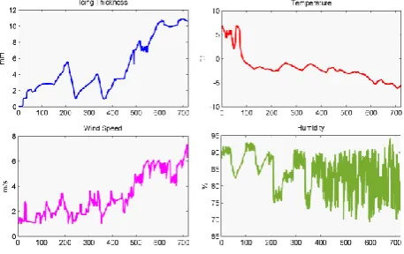
Data are chosen from the data monitoring center of key laboratory of anti-ice disaster. A 500kV overhead transmission line called “Zhe-Ming line”, located in Hunan Province, China, is chosen as real-world case study. The icing data points are collected every fifteen minutes from 0:00 on 1/4/2009 to 11:45 on 1/11/2009, which total up to 720 data points, as shown in Fig.3. The former 576 data points are used as training sample, and the last 144 as testing sample. Furthermore, the main micro-meteorology data, including temperature, humidity, wind speed, are still shown in Fig.3. Hunan Province is located in the middle and lower reaches of the Yangtze River and in the south of the Dongting Lake, surrounded by mountains on three sides, the Xiangzhong basin mainly includes hills, mounds, and valley alluvial plains. The terrain is very conductive for winter strong cold air to march from the North, and the Nanling stationary front is formed at the confluence of the cold air and the South China Sea subtropical warm air in the north slope of Nanling mountains. In the areas covered with the stationary front, the super-cooled water in the condensation layer is very unstable, and extremely easy to adhere to the relatively cold hard objects such as wires to form the rime and glaze. In 2008, Hunan power grid suffered a severe freezing damage, which caused many incidents such as towers collapse, lines breakage, ice flash, tripping, etc., leading to a large scale blackout disaster. The freezing time, covering area and icing conditions of this damage had been the most serious since 1954. Therefore, the high voltage transmission lines in Hunan Province are selected as case studies, which has a certain universality.

Figure.3 Original data chart of icing thickness, temperature, wind speed and humidity

scaled to the range [0, 1] by using their maximum and minimum values. Finally, it should be noted that the predicted values must be re-scaled back by using the reverse formula in order to guarantee the convenience and maneuverability for the results analysis. The scaled formula of sample data is shown as follows:

 

i n

y y

y y z

Z i

i 1,2,3,...,

min max

min 

  

 ₍₂₇₎

Whereymaxandyminare the maximum and minimum value of sample data, respectively.

4.3 Fireworks algorithm for feature selection

In this section, we use fireworks algorithm to obtain the final optimal feature subset. The environment used for feature selection include Matlab R2013a, self-written Matlab program and a computer with the Intel(R) Core(TM)2Duo CPU, 3GB RAM and Windows7 Professional operation system. The parameters of fireworks algorithm are set as follows: the maximum iteration number

500



Maxgen _{, the population size} PopNum30_{, the constant determining the number of sparks} 100



M , the constant determining the explosion radius Rˆ150, the upper and lower limits of the individual searching range of fireworks areV_up 512 _andVdown512respectively. The parameters of W-LSSVM are chosen as follows:



23.698_,  5.123.

Figure.4 The curve of convergence and global optimum

Figure.4 is the iterative process curve of fireworks algorithm for the sample data. As the figure is shown, the fitness curve describes the best fitness value which is obtained by the FA model at each iteration; the accuracy curve is the value which is calculated by the W-LSSVM model at different iterations; the reduced No is the number of eliminated features in the process of convergence; and the selected No is the number of obtained features in every iteration with the new method. As we can see from the Fig.4, the optimal fitness value is -0.93, which is found by FA when the iterative number reaches 46. In the 46th iteration, the prediction accuracy based on training sample meets the best of 98.8%; which means the machine learning of W-LSSVM achieves the best and obtains the highest predictive accuracy in the training sample data. Furthermore, the number of selected features is stable when the iterative number is 46, and we can see that 15 features are eliminated from original 20 features. The final selected features for the sample are temperature, humidity, wind speed, sunlight intensity and air pressure, respectively.

4.4 W-LSSVM for icing forecasting

In order to prove the performance of the proposed forecasting model for icing thickness, three well-known icing forecasting models including SVM (support vector machine), BPNN (BP neural networks) and MLRM (multi-variable linear regression model) are also applied to the data-set described in Section 4.2. In the single SVM forecasting model, the parameters are chosen as follows:

913 . 10



C _,





0

.

0012

_,



2.4532_.

In the BPNN icing forecasting model, the number of input layer, hidden layer and output layer are 5, 7, and 1 respectively. The Sigmoid function is selected as the transfer function. The maximum permissible error of model training is 0.001, and the maximum training time is 5000.

Furthermore, this paper will use the relative error (RE), mean absolute percentage error (MAPE), and root mean square relative error (RMSE) as the final evaluation indicators:

% 100 )

( ) ( ˆ )

(  _



i y

i y i y

RE (28)

% 100 )

( ) ( ˆ ) ( 1

1

 







N

i yi

i y i y N

MAPE (29)







 N

i y i

i y i y N RMSE

1

2

) ) (

) ( ˆ ) ( ( 1

(30)

Where

y

(

i

)

is the original icing thickness value, and

y

ˆ

(

i

)

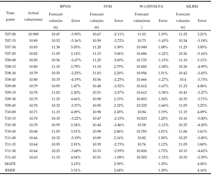
is the predictive value.

All the icing thickness forecasting value with the BP, SVM, W-LSSVM-FA and MLRM models are shown in Fig.5, part of which are given in Table 2. In addition, Fig.6 gives the forecasting errors with these models. Based on the above results, several patterns are observed.

Firstly, the maximum and minimum gap between original icing value and forecasting value are captured from the Fig.5. In MLRM model, the maximum gap is 0.77 mm, and minimum gap is 0.25 mm. In BPNN model, the maximum and minimum gap are 0.56 mm and 0.16 mm, respectively. Both values of BPNN are smaller than that of MLRM, which indicates that the forecasting accuracy of BPNN is much more precise. In the single SVM model, the maximum and minimum gap are 0.47 mm and 0.11 mm, respectively. The deviation between the maximum and minimum gap of single SVM model is 0.36mm, which is smaller than that of BPNN and MLRM; this result demonstrates that SVM icing forecasting model is much more stable than that of BPNN and MLRM. In the proposed W-LSSVM-FA model, the maximum gap is only 0.2 mm and the minimum gap is only 0.064 mm. Compared with other three models, both values of W-LSSVM-FA are smaller and the deviation between the maximum and minimum gap is 0.136 mm, which is also smaller than that of SVM, BPNN and MLRM. This illustrates that the proposed W-LSSVM-FA model has a higher prediction accuracy and stability.

Figure.5 The forecasting value of the proposed method

the forecasting accuracy and the nonlinear fitting ability of BPNN is stronger than that of MLSM. In the single SVM model, the maximum and minimum errors are 4.7% and 1.09%; both values of SVM are superior to that of BPNN and MLRM, and the fluctuating range of RE curve of SVM is rather smaller. This again demonstrates the accuracy and the stability of SVM are higher than that of BPNN and MLRM in icing forecasting. In the proposed W-LSSVM-FA model, the maximum and minimum relative errors are 1.94% and 0.64%, respectively. Both of the values are the smallest among BPNN, SVM, MLRM model. Moreover, the fluctuation of the curve is small, which is superior to the other models. Compared with other three models, the proposed W-LSSVM-FA icing forecasting model has a higher accuracy and stability. Owing to that it makes a great pretreatment on the data with the input vectors weighted and that some redundant factors have been eliminated through the feature selection, the forecasting accuracy is improved, and the machine learning and training ability are relatively strengthened.

Table 2 The forecasting values and errors of each model

Time point

Actual value(mm)

BPNN SVM W-LSSVM-FA MLRM

Forecast value(m

m)

Error

Forecast value(m

m)

Error

Forecast value(mm

)

Error

Forecast value(m

m)

Error

T07-00 10.900 10.47 -3.95% 10.67 -2.11% 11.03 1.19% 11.25 3.21%

T07-15 10.89 10.52 -3.36% 10.59 -2.72% 10.73 -1.43% 10.54 -3.18%

T07-30 10.83 11.38 5.05% 11.20 3.39% 10.949 1.08% 11.25 3.85%

T07-45 10.82 11.05 2.14% 11.15 3.06% 10.686 -1.22% 10.26 -5.16%

T08-00 10.85 10.56 -2.67% 11.25 3.69% 10.725 -1.15% 11.19 3.12%

T08-15 10.80 11.10 2.79% 11.10 2.79% 10.682 -1.08% 10.26 -4.99%

T08-30 10.79 10.55 -2.25% 11.03 2.20% 10.956 1.51% 10.42 -3.45%

T08-45 10.80 10.35 -4.19% 10.56 -2.25% 10.666 -1.27% 10.4 -3.73%

T09-00 10.79 10.95 1.47% 10.48 -2.92% 10.612 -1.67% 11.23 4.06%

T09-15 10.78 11.02 2.20% 10.51 -2.57% 10.612 -1.58% 10.43 -3.27%

T09-30 10.75 11.25 4.66% 10.98 2.15% 10.893 1.34% 10.35 -3.71%

T09-45 10.70 10.32 -3.57% 10.95 2.32% 10.525 -1.66% 11.05 3.25%

T10-00 10.71 11.15 4.09% 10.98 2.45% 10.84 1.19% 11.15 4.09%

T10-15 10.70 10.35 -3.22% 10.47 -2.15% 10.823 1.20% 10.16 -5.00%

T10-30 10.70 10.95 2.34% 10.44 -2.46% 10.58 -1.12% 10.25 -4.20%

T10-45 10.68 11.05 3.51% 10.98 2.86% 10.783 1.01% 11.06 3.61%

T11-00 10.66 10.32 -3.19% 10.89 2.16% 10.82 1.50% 10.25 -3.85%

T11-15 10.64 10.95 2.91% 10.35 -2.73% 10.76 1.12% 11.05 3.80%

T11-30 10.64 10.25 -3.68% 10.33 -2.93% 10.826 1.73% 10.15 -4.62%

T11-45 10.63 11.15 4.94% 10.51 -1.09% 10.503 -1.15% 10.35 -2.59%

MAPE 3.23% 2.59% 1.35% 4.06%

RMSE 3.31% 2.68% 1.38% 4.16%

Figure.6 The relative errors curve of each method

Thirdly, the forecasting results can be evaluated by calculating the MAPE and RMSE. As the calculation results are shown, the MAPE values of W-LSSVM-FA, SVM, BPNN and MLRM models are 1.35%, 2.59%, 3.23% and 4.06%, respectively. The proposed W-LSSVM-FA model has a lower error than the other models. RMSE value is used to evaluate the discrete degree of whole forecasting values of each model. As we see in Table 2, the RMSE values of W-LSSVM-FA, SVM, BPNN and MLRM are 1.38%, 2.68%, 3.31%, and 4.16%, respectively. The discrete degree of W-LSSVM-FA icing forecasting model is the lowest, this demonstrates the proposed W-LSSVM-FA model is more stable for the prediction of icing thickness, and it can reduce the redundant influence of irrelevance factors through feature selection.

4.5. Further simulation

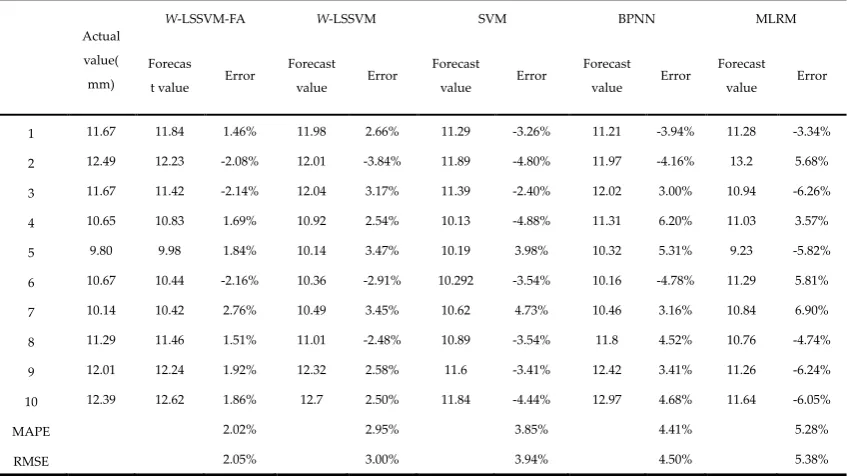
To verify whether the W-LSSVM can bring better results, another representative 500kV high voltage transmission line, called “Fusha-Ӏ-xian”, is selected to make an comparison of the forecasting results by using the selected features (W-LSSVM-FA method) and original features (only W-LSSVM method). The sample data of “Fusha-Ӏ-xian” are also predicted by BPNN, SVM, MLRM and the results of five models are also used to make a comparison. Part of the original data, which totally have 287 data groups, are shown in Figure 7. The former 247 data points are used as training sample, and the last 40 as testing sample.

In the W-LSSVM-FA model, use FA model to select the features, and the iterative process curve of fireworks algorithm for the sample data of “Fusha-Ӏ-xian” is shown in Fig.8. As we can see from the Fig.8, the optimal fitness value is -0.916, which is found by FA when the iterative number reaches 55. The final selected features for the sample are temperature, humidity, wind speed, wind direction and sunlight intensity, respectively. And the parameters of W-LSSVM are obtained as follows:  56.7841_,



14.7715. In W-LSSVM model, the original features are just temperature, humidity and wind speed. With the method of cross validation, the parameters of W-LSSVM are obtained as follows:



38.9962,  15.3720.

Figure.8 The iteration curve for the sample data of “Fusha-Ӏ-xian”

All forecasting results and the relative errors of five models are shown in Fig.9 and Fig.10, respectively. A part of forecasting values and errors of five models are listed in Table 3.

The MAPE and RMSE values of the five models are shown in Table 3. It can be seen that the proposed W-LSSVM-FA model still has the smallest MAPE and RMSE values, which are 2.02% and 2.05%, respectively. This again reveals the proposed W-LSSVM-FA model has the best performance in icing thickness forecasting.Moreover, the MAPE and RMSE values of W-LSSVM are smaller than that of SVM, BPNN and MLRM, this demonstrates the W-LSSVM has a higher prediction accuracy and better learning ability by using original features to forecast.

As is shown in Fig.9, the prediction values of W-LSSVM-FA are closest to the original values, this again proves the W-LSSVM-FA model has a higher forecasting accuracy and stability compared with other four prediction models. The prediction results of W-LSSVM are closer to the original data than that of SVM, BPNN, MLRM model, this again reveals that it can improve the nonlinear mapping ability and strength the learning ability of the machine through weighting process of LSSVM.

Table 3 Part of the forecasting values and relative errors of each model

Actual

value(

mm)

W-LSSVM-FA W-LSSVM SVM BPNN MLRM

Forecas

t value Error

Forecast

value Error

Forecast

value Error

Forecast

value Error

Forecast

value Error

1 11.67 11.84 1.46% 11.98 2.66% 11.29 -3.26% 11.21 -3.94% 11.28 -3.34%

2 12.49 12.23 -2.08% 12.01 -3.84% 11.89 -4.80% 11.97 -4.16% 13.2 5.68%

3 11.67 11.42 -2.14% 12.04 3.17% 11.39 -2.40% 12.02 3.00% 10.94 -6.26%

4 10.65 10.83 1.69% 10.92 2.54% 10.13 -4.88% 11.31 6.20% 11.03 3.57%

5 9.80 9.98 1.84% 10.14 3.47% 10.19 3.98% 10.32 5.31% 9.23 -5.82%

6 10.67 10.44 -2.16% 10.36 -2.91% 10.292 -3.54% 10.16 -4.78% 11.29 5.81%

7 10.14 10.42 2.76% 10.49 3.45% 10.62 4.73% 10.46 3.16% 10.84 6.90%

8 11.29 11.46 1.51% 11.01 -2.48% 10.89 -3.54% 11.8 4.52% 10.76 -4.74%

9 12.01 12.24 1.92% 12.32 2.58% 11.6 -3.41% 12.42 3.41% 11.26 -6.24%

10 12.39 12.62 1.86% 12.7 2.50% 11.84 -4.44% 12.97 4.68% 11.64 -6.05%

MAPE 2.02% 2.95% 3.85% 4.41% 5.28%

Figure.9 The forecasting values of each model

The relative errors can be seen in Fig.10. We can see from the above computation that comparing with the W-LSSVM-FA and W-LSSVM method, the W-LSSVM-FA model has higher forecast precision. And in W-LSSVM model, the relative errors are more fluctuant compared with W-LSSVM-FA, it can also be seen that using W-LSSVM-FA model to forecast has better stability and accuracy than the W-LSSVM model. Because it can select different features and remove many unrelated factors that make no or little effect on icing forecasting with the fireworks algorithm optimization. Moreover, the use of feature selection with FA can greatly ensure the integrity of the information for different data characteristics, which makes the prediction accuracy of W-LSSVM-FA much higher. On the contrary, the use of original features to forecast is impossible to ensure information completeness for the different data, which may degrades the prediction precision.

In summary, the proposed W-LSSVM-FA can reduce the forecasting errors between original icing thickness values and predictive values. It can reduce the influence of unrelated noises with feature selection based on fireworks algorithm. The LSSVM model improves its nonlinear mapping ability with horizontal and vertical weighting, and its training and learning ability has been strengthen very well in this way. The numerical experimental results have demonstrated the feasibility and effectiveness of the proposed W-LSSVM-FA icing forecasting method.

Figure.10 The relative errors of each model

5 Conclusions

utilized to make the feature selection for eliminating the redundant influence of many uncertain factors in icing forecasting. Considering the specific combination optimization problem based on FA, the initial feature subsets are determined by calculating the correlation coefficient. In order to improve the generalization and learning ability of the algorithm, the LSSVM is improved though the horizontal and vertical weighting. After automatically obtaining the inputs, the WLSSVM is used to train and test the data. According to the results of simulation for the Zhe-Ming transmission line, the proposed W-LSSVM-FA model can find the optimal feature subsets and achieve the expected accuracy. Furthermore, by comparing it with three classical icing forecasting models (SVM,BPNN and MLRM), the proposed W-LSSVM-FA model has shown superior performance in terms of RE, MAPE and RMSE. Therefore, it can be concluded that the proposed model might be an alternative for icing forecasting.

Acknowledgments: This work is supported by the Natural Science Foundation of China (Project No. 71471059).

References

[1] Xu X, Niu D, Wang P, et al. The Weighted Support Vector Machine Based on Hybrid Swarm Intelligence Optimization for Icing Prediction of Transmission Line[J]. Mathematical Problems in Engineering, 2015, 501: 798325.

[2] Musilek P, Arnold D, Lozowski E P. An ice accretion forecasting system (IAFS) for power transmission lines using numerical weather prediction[J]. SOLA, 2009, 5: 25-28.

[3] Li Q, Li P, Zhang Q, et al. Icing load prediction for overhead power lines based on SVM[C]//Modelling, Identification and Control (ICMIC), Proceedings of 2011 International Conference on. IEEE, 2011: 104-108. [4] Huang X, Li J. Icing thickness prediction model using BP Neural Network[C]//Condition Monitoring and Diagnosis (CMD), 2012 International Conference on. IEEE, 2012: 758-760.

[5] Zarnani A, Musilek P, Shi X, et al. Learning to predict ice accretion on electric power lines[J]. Engineering Applications of Artificial Intelligence, 2012, 25(3): 609-617.

[6] Liu C, Liu H W, Wang Y S, et al. Research of icing thickness on transmission lines based on fuzzy Markov chain prediction[C]//Applied Superconductivity and Electromagnetic Devices (ASEMD), 2013 IEEE International Conference on. IEEE, 2013: 327-330.

[7] Sheng C, Dong D, Xiaotin H, et al. Short-term Prediction for Transmission Lines Icing Based on BP Neural Network[C]//Power and Energy Engineering Conference (APPEEC), 2012 Asia-Pacific. IEEE, 2012: 1-5.

[8] Du X, Zheng Z, Tan S, et al. The study on the prediction method of ice thickness of transmission line based on the combination of GA and BP neural network[C]//E-Product E-Service and E-Entertainment (ICEEE), 2010 International Conference on. IEEE, 2010: 1-4.

[9] Peng L, Qimao L, Min C, et al. Time series prediction for icing process of overhead power transmission line based on BP neural networks[C]//Control Conference (CCC), 2011 30th Chinese. IEEE, 2011: 5315-5318.

[10] Huang X B, Li J J, Ouyang L S, et al. Icing Thickness Prediction Model Using Fuzzy Logic Theory[J]. Gaodianya Jishu/ High Voltage Engineering, 2011, 37(5): 1245-1252.

[11] Shifeng Y, Yong L, Zha W, et al. Icing Thickness Forecasting of Overhead Transmission Line under Rough Weather Based on CACA-WNN[J]. Electric Power Science and Engineering, 2012, 11: 007.

[12] LIU Jun, LI An-jun,ZHAO Li-ping. A prediction model of ice thickness based on T-S fuzzy neural networks[J]. HUNAN ELECTRIC POWER,2012,32(3):1-4

[13] YING Zi-ren, SU Xiao-lin. Icing Thickness Forecasting of Transmission Line Based on Particle Swarm Algorithm to Optimize SVM[J]. JOURNAL OF ELECTRIC POWER,2014,29(1):6-9.

[14]Huang xiao-ting, Xu Jia-hao, et al. Transmission line icing prediction based on data-driven algorithm and LS-SVM[J].Automation of Electric Power System,2014,38(15):81-86

[15] Dai Dong, Huang Xiao-ting, et al. Regression model for transmission lines icing based on support vector machine[J].High Voltage Engineering,2013,39(11):2822-2828.

[16] ElAlami M E. A filter model for feature subset selection based on genetic algorithm[J]. Knowledge-Based Systems, 2009, 22(5): 356-362.

[17] Hu Z, Bao Y, Chiong R, et al. Mid-term interval load forecasting using multi-output support vector regression with a memetic algorithm for feature selection[J]. Energy, 2015, 84: 419-431.

[18]Zhao Zhi-mei. Feature selection algorithm based on surrogate model and artificial immune system[J].COMPUTER ENGINEERING AND DESIGN,2014,35(6):2174-2178

algorithm[C]//Computational Sciences and Optimization, 2009. CSO 2009. International Joint Conference on. IEEE, 2009, 2: 969-973.

[20] Bae C, Yeh W C, Chung Y Y, et al. Feature selection with intelligent dynamic swarm and rough set[J]. Expert Systems with Applications, 2010, 37(10): 7026-7032.

[21] Aghdam M H, Ghasem-Aghaee N, Basiri M E. Text feature selection using ant colony optimization[J]. Expert systems with applications, 2009, 36(3): 6843-6853