Statistical Theory of Plasmas Turbulence
∗)Eun-jin KIM and Johan ANDERSON
Department of Applied Mathematics, University of Sheffield, Sheffield, S3 7RH, U.K. (Received 31 August 2008/Accepted 20 April 2009)
We present a statistical theory of intermittency in plasma turbulence based on short-lived coherent structures (instantons). In general, the probability density functions (PDFs) of the fluxRare shown to have an exponen-tial scalingP(R)∝exp (−cRs) in the tails. In ion–temperature–gradient turbulence, the exponent takes the value s=3/2 for momentum flux ands=3 for zonal flow formation. The value ofsfollows from the order of the high-est nonlinear interaction term and the moments for which the PDFs are computed. The constantcdepends on the spatial profile of the coherent structure and other physical parameters in the model. Our theory provides a pow-erful mechanism for ubiquitous exponential scalings of PDFs, often observed in various tokamaks. Implications of the results, in particular, on structure formation are further discussed.
c
2009 The Japan Society of Plasma Science and Nuclear Fusion Research
Keywords: turbulence, structure, shear flow, confinement, probability density function (PDF) DOI: 10.1585/pfr.4.030
1. Introduction
The need for statistical theory of plasma turbulence has grown significantly over the past decade with accumu-lating evidence from simulation and experiments showing highly intermittent and bursty turbulent transport [1–9]. Probability density functions (PDFs) inferred from these experiments are strongly non-Gaussian, particularly in the tails, due to rare events of large amplitude. For instance, exponential scalings appear to be a robust feature of the tails of heat, particle, and momentum fluxes in a variety of tokamaks (for example, [10–13]). These observations suggest that Gaussian statistics and average transport coef-ficients based on mean field theory fail to capture essential transport processes of intermittency and demand a proper nonlinear theory for events of large amplitude. Given the potentially disastrous impact of these events on confine-ment, the importance of a predictive theory of PDF tails cannot be overemphasized.
While these coherent structures mediate significant transport, as mentioned above, they can also play a com-plementary role in inhibiting transport via enhanced decor-relation. Improvements in plasma confinement by mean flows and zonal flows [14] are notable examples. Given the importance of such structures in intermittency and transport, the PDF of the formation of the structure itself is a quantity of ultimate interest. For instance, an interest-ing issue is the prediction of the PDF of the L→H transi-tion [15].
This paper presents a non-perturbative theory of PDFs in plasma turbulence and investigates the structure forma-tion — in particular, zonal flow formaforma-tion. Our theory
author’s e-mail: e.kim@shef.ac.uk
∗) This article is based on the invited talk at the 14th International Congress on Plasma Physics (ICPP2008)
is motivated by the following key experimental observa-tions. The first is that coherent structures (which tend to form naturally in nonlinear systems) mediate fast transport and are responsible for the intermittency in the PDFs. The second is that coherent structures tend to be short-lived in time, causing bursty events (for example, [12, 13]). Ex-amples of such short-lived structures include streamers, blobs, and vortices. This empirical fact that short-lived coherent structures are responsible for intermittency and PDF tails is precisely built into our theoretical tool: the so-called “instanton method.” Section 2 provides a few brief comments on the method. Sections 3 and 4 describe the use of this method to develop a non-perturbative theory of the PDFs of structure formation in the ion–temperature– gradient (ITG) model. Section 5 presents a discussion and conclusions.
2. Instantons
This section provides historic background on instan-tons to help readers understand their physical significance and why they are useful for the development of a statistical theory of turbulence. Instantons originated in quantum me-chanics as a non-perturbative way of computing the transi-tion amplitude from one ground state to another [16]. The basic idea is that the uncertainty relationship between posi-tion and momentum allows one to formulate the transiposi-tion amplitude from the initial positionxi to the final position
xf by a path integral as follows (see Fig. 1):
xf|eiHT/|xi=N
x=xf
x=xi
Dx(t)eiS/,
whereS = dtmv2/2−U(x)is action, andH=mv2/2+
U(x) is a Hamiltonian with potentialU. We can expand the left side of the equation in terms of a complete set of
c
2009 The Japan Society of Plasma
Fig. 1 Trajectories of a particle between initial position xi at
timet=0 and final positionxfatt=T.
energy eigenstates to obtain xf|eiHT/|xi=
n
xf|EnEn|xieiEnT/.
The previous equation implies that the transition ampli-tude from one ground state to another can be isolated by taking time to be imaginary. Expressed in terms of imaginary time, action becomes “Euclidean action”SE =
dt[mv2/2 +U]. An instanton is a saddle-point
solu-tion of Euclidean acsolu-tion and corresponds to one particular path that leads to the transition amplitude between ground states. For instance, in the case of double-well potential, an instanton is a tunneling solution from the bottom of one potential well to another (see Fig. 2 (a)). If a solution go-ing from one ground state to the other is called an instan-ton, a solution traveling in the opposite direction is called an anti-instanton. As noted above, a distinguishing char-acteristic of such solutions is temporal localization (see Fig. 2 (b)). The instanton method was used in gauge field theory to compute the transition amplitude from one vac-uum to another vacvac-uum [17]. About 20 years later, the method was adapted to a classical fluid problem by several authors [18–21].
3. PDF Tails in Plasma Turbulence
Armed with general concepts of instantons, in this section, we develop a general theory of PDFs in plasma tur-bulence. In plasma turbulence, unpredictability can arise either from the chaos intrinsic to the system or from an ex-ternal random forcing. Between the two, clearly, it is much easier to formulate a PDF in the case of an external forc-ing, to which the following discussion is limited. In fact, it is well known that a similar path integral can be formu-lated for stochastic equations with a random external forc-ing [22, 23]. For instance, the effective action for classical forced systems was formulated by Martin, Sigga, and Rose in 1973 [24]. However, the non-perturbative evaluation of a path integral had to wait until the (non-perturbative) saddle-point (instanton) method was used to compute the tail of the PDF [18, 19].
Fig. 2 (a) Double-well potential with a particle sitting at the bot-tom of a potential well. A particle going fromx=−ato ais an instanton; a particle going fromx=ato−ais an anti-instanton. (b) Position of a particle as a function of time, traveling betweenx=−aanda. The positive (neg-ative) slope corresponds to an instanton (anti-instanton).
We consider a prototype nonlinear dynamical system driven by an external (stochastic) forcing f
∂tφ+N(φ)= f, (1)
whereN(φ) represents the sum of linear and nonlinear in-teractions with the highest nonlinearity ofn. For simplic-ity, we take the statistics of the forcing in Eq. (1) to be Gaussian with delta-correlation in time as follows:
f(x,t)f(x,t) = δ(t−t)κ(x−x), (2) andf=0. For Gaussian statistics with a vanishing first moment, the prescription for the second moment given by Eq. (2) is sufficient, simply because all odd moments van-ish while even moments can be expressed as a product of second moments. Note that, even if the forcing is Gaus-sian,φstatistics can be Gaussian because of the non-linearity of the dynamical equation. An equivalent way of prescribing the second moment (Eq. (2)) for the Gaussian forcing is to introduce the PDF off as follows [23]:
d[ρ(f)]=Dfe−12
dxdxdt f(x,t)κ−1(x,x)f(x,t)
. (3) This is a generalization of a Gaussian distribution to a con-tinuous variablef(x,t). The average value of a quantityQ is then computed as
Q=
where the angle bracketsrepresent the average over the statistics of the forcing f. From Eq. (3), we construct the PDFs of flux, which are themmultiple products ofφ (that is, themth moment). In the following, we callM(φ) the “observable,” since we are interested in measuring its PDFs. The PDFs ofM(φ) to take a value ofRcan then be represented in terms of a path integral as follows:
P(R) = δ(M(φ)−R)
=
dλeiλR
e−iλM[φ]
=
dλeiλR
Iλ, (5)
where
Iλ=
e−iλM[φ].
By taking Q[φ] = exp [−iλM[φ]] in Eq. (4) and using Eq. (3), we can rewriteIλin terms of a path integral as
Iλ =
DφDφe−Sλ, (6)
whereSλis the effective action given by Sλ = −i
dxdtφ[∂tφ+N(φ)]
+ 1
2
dxdxdtφ(x)κ(x−x)φ(x)
+ iλ
dtM(φ)δ(t). (7)
In Eq. (7),φ is the conjugate variable toφ, introduced to impose the constraint given by the equation of motion ofφ in Eq. (1) in the form
N=
Dφexp i
dxdtφ[∂tφ+N(φ)−f]
,
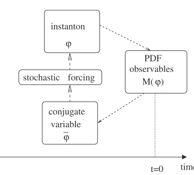
with a normalization constantN. Althoughφappears to be simply a convenient mathematical tool, it does have a use-ful physical meaning: it arises from the uncertainty in the value ofφdue to stochastic forcing. That is, the dynami-cal system with a stochastic forcing should be extended to a larger space involving this conjugate variable, whereby φandφconstitute an uncertainty relationship (see Fig. 3). The instanton solution is a particular path out of all pos-sible (functional) values ofφ andφwhich minimizes the actionSλ. Furthermore, the conjugate variables have the interesting physical property of mediating the forcingκand the fluxM(φ) (oberservable) whose PDFs are sought (see Fig. 4).
3.1
Instanton solution
The key concept underlying the instanton method is that coherent structures that are localized in time are re-sponsible for the rare events of large amplitude, causing strong intermittency in the PDF tails with possibly signifi-cant transport. Assuming that such a coherent structure has a spatial profileφ0(x) and a temporal evolution governed
Fig. 3 Uncertainty inφ=F(t)φ0andφ=μ(t)φ(or inF(t) and
μ(t)) due to stochastic forcing.
Fig. 4 Schematic diagram showing the relationship among the PDFs of the observable M(φ), dynamical quantityφ, its conjugate variableφ, and the stochastic forcing with the correlation functionκ(x−x) (see Eq. (2)).
byF(t) asφ(x,t)=φ0(x)F(t), and similarlyφ=φ0(x)μ(t),
we can rewrite the actionSλand minimize it with respect to F and μ to obtain equations for F and μ. Since the instantonφpropagates forward in time and its conjugate variableφbackward in time while the PDF is computed at t = 0, the boundary conditions on F andμare (see also Fig. 3):
F(−∞)=0, (8)
μ(t>0)=0. (9) To make further progress, we need to specify the profile of φ0. The key question is thus “what should we use
for φ0?” or, alternatively, “what are the possible
and expanding the correlation functions in terms of those as
κ(x−y)∼κ0
m,n
φm 0(x)φ
n 0(y),
whereκ0 is the strength of forcing, we can, in principle,
cast the action in terms of a time-integral only. Schemati-cally, computation of the PDFs then requires the following main steps:
I. Minimize Sλ with respect to μ and F to obtain the equation of motion forFandμ.
II. Solve those equations with the boundary conditions (Eqs. (8) and (9)) to compute optimal paths.
III. Use those solutions to obtain the minimum actionSλ. IV. Evaluateλintegral in Eq. (5) to find the PDFs.
4. PDFs of Structure Formation in
ITG Turbulence
This section predicts the PDFs of structure formation in ITG turbulence by the preceding steps. As a specific ex-ample, we investigate the PDFs of the formation of zonal flows. Since zonal flows are self-driven from turbulence by Reynolds stress, this problem is closely related to the PDF of momentum flux. We thus consider the PDFs of momentum transport and zonal flow formation. The PDFs of the local Reynolds stress in Hasagawa-Mima [25, 26] and toroidal ITG turbulence models were investigated by Kimet al. [27, 28]. In the following, we consider a slightly different ITG model and compute the PDFs of (global) mo-mentum flux and zonal flow formation [29, 30]. Specifi-cally, we model ITG turbulence using the continuity and temperature equation for the ions, assuming Boltzmann electrons, and ignoring the effects of parallel ion motion, magnetic shear, trapped particles, and finite beta on the ITG modes [31]. We incorporate the effect of an imposed poloidal shear flow in the time-evolution equations for the background fluctuations in the form of sheared velocityV0.
The main governing equations are given by ∂tn−
∂t−αi∂y
∇2
⊥φ+∂yφ+φ,n+ν∇4φ
+V0∂y
1− ∇2⊥φ−ngi∂y(φ+τ(n+Ti))
=φ,∇2 ⊥φ
+τφ,∇2
⊥(n+Ti)
+f,
(∂t+V0∂y)Ti−
5
3τngi∂yTi+
ηi−
2 3
∂yφ
−2
3(∂t+V0∂y)n=−[φ,Ti]+ 2 3[φ,n].
(10) Here, f is the forcing, and V0 is an imposed shear flow.
Notations are standard: [A,B]=(∂xA)(∂yB)−(∂yA)(∂xA); n = (Ln/ρs)δn/n0 is the normalized ion particle density;
φ = (Ln/ρs)eδφ/Te is the eletrostatic potnetial; Ti =
(Ln/ρs)δTi/Ti0the ion temperature;τ=Ti/Te;ρs=cs/Ωci
where cs =
√
Te/mi; Ωci = eB/mic; ν is
collisional-ity; LT = −(dlnT/dr)−1, andLn = −(dlnn/dr)−1; ηi =
Ln/LTi, n = 2Ln/R¯ where ¯R is the major radius; and
αi=τ(1+ηi). Length scale and time are normalized byρs
andLn/cs, respectively. The geometrical quantities are
cal-culated in the strong ballooning limit (θ=0,gi(θ=0)=1,
withω = kyv = ρscsky/Ln). Physically, the forcing f
is envisioned to arise from the instability of toroidal ITG modes due to unfavorable magnetic curvature, or an exter-nal particle source.
We assume that a coherent structure responsible for the PDF tails has the spatial profile given by modons prop-agating with speedU in the local poloidaly direction as φ0(x, y) = φ0(x, y −Ut) (for example, [26]).
Further-more, we assume a linear relationship betweenφ andTi
asTi=χφwith
χ= ηi−
2
3(1−U+V0)
U−V0+53τngi
.
The coupled equations (10) then effectively reduce to one equation forφwith the nonlinear interaction termN[φ] in Eq. (7) given by
N[φ]=−(∂t−αi∂y)∇⊥2φ+V0(1− ∇2⊥)φ
+(1−ngiβ)∂yφ−β[φ,∇2⊥φ]+ν∇4φ, (11)
whereβ=1+τ+τχ. By substituting Eq. (11) inSλand usingφ = F(t)φ0, we obtain the effective actionSλas a
function ofF(t) and ¯φ(x,t). We note that for a nonlinear modon solution to exist, the ITG mode should be linearly unstable (for example, [32]).
4.1
Momentum flux
We first consider the observable to be momentum flux M[φ]=vxvy=
−∂φ∂
x ∂φ ∂y
, (12)
where angle bracketsdenote spatial average, and com-pute the PDFs of the momentum fluxM[φ] to take a value ofR(that is,P(R)).
By substituting Eq. (12) into Sλ Eq. (7) with φ = F(t)φ0, and following Sect. 3 Steps I-IV, we obtain the
de-sired PDFs of the momentum fluxP(R) as
P(R) ∼ exp{−c1R3/2}, (13)
where c1 is a constant that depends on the profile of the
coherent structure (modon) and the values of the physi-cal parameters (U−V0,ηi,τ, etc). Equation (13) clearly
shows that the PDF tails are strongly intermittent with ex-ponential scaling exp (−cR3/2). Our prediction thus offers
a powerful mechanism for ubiquitous exponential scal-ings observed experimentally (for example, [10–13]). No-tably, exactly the same exponential scaling exp (−cR3/2) of
Reynolds stress was reported in [11]. Of particular impor-tance, we find that the PDF is enhanced over the Gaussian prediction exp (−cR2), highlighting the importance of
in-termittency in understanding momentum transport. Simi-lar exp (−cR3/2) was also obtained in the PDFs of local
ITG turbulence models [27,28]. These results follow from the fact that (i) the highest nonlinearity in our model is quadratic and (ii) the observable is the second-order mo-ment (momo-mentum flux) [33]. Were it not for a linear re-lationship betweenTiandφ, a different exponential
scal-ing would have followed. On the other hand, the constant c1 depends on the spatial profile of the coherent structure
(modons), U−V0, and other physical parameters (ηi,τ,
etc.), which is investigated in detail in [30].
4.2
Zonal flow formation
We consider zonal flows, driven by Reynolds stress (momentum flux), as
∂φZF(t)
∂t =−vxvy. (14) To include the dynamics of zonal given in Eq. (14), we need to introduce the conjugate variable for zonal flows as ¯φZF. The additional contribution from zonal flows to the
actionSλis then given by
ΔSλ=−i
dtφ¯ZF(t)
∂φ
ZF(t)
∂t +vxvy
. (15)
To compute the PDFs of zonal flows, we consider the ob-servable to be zonal flows
M[φZF]=φZF. (16)
By incorporatingΔSλ(Eq. (15)), substituting Eq. (16) into Eq. (7), and following Sect. 3 Steps I-IV, we obtain PDFs of zonal flows to take the value ofR(that is,P(R)) as fol-lows:
P(R) ∼ exp{−c2R3}. (17)
Here,c2 is the model-dependent constant that determines
the amplitude of the PDFs. The exponential scaling in Eq. (17) again indicates a strong intermittency in the tails. The exact scaling here follows from the fact that (i) the highest nonlinearity in our model is quadratic and (ii) the observable is the first order moment (zonal flow). Note that, for the same reason, a similar exp (−cR3) scaling was found in the tails of the PDFs of positive velocity gradients in Burgers turbulence [18]. While the exponential scaling is robust, the amplitude of the PDFs rather sensitively de-pends on parameter values in the model through the value of the constantc2 [30, 33]. Similar exponential PDFs are
thus expected when the effect of toroidal coupling is incor-porated, with the same (quadratic) highest nonlinearity in Eq. (10). The toroidal effect will however change the over-all amplitude of PDFs by effectively altering the forcing strength (κ0).
Note that, in this model, the back reaction of zonal flows is neglected, by assuming an imposed shear flow. Computation of the PDFs in a more consistent model is in progress where zonal flows are treated dynamically by allowing them to modify the evolution of fluctuations. Fi-nally, note that a simplified 1D model for a shear flow
has been proposed in terms of a nonlinear diffusion equa-tion, where a shear flow is driven by a stochastic forcing while damped through a nonlinear diffusion of the form D(ux)=γu2x[34]. Here,ux=∂xu;γis constant. Analysis
of this model was recently done by [35].
4.3
Summary
The instanton method predicts exponential PDFs of momentum flux (second moments) and structure formation (first moments) with exp (−cR3/2) and exp (−c2R3)
scal-ings, respectively. Our theory thus explains similar ex-ponential PDF tails often observed in various tokamaks [11–13]. Furthermore, we can show that PDFs of higher moments such asnvxvy have exponential PDFs that are
much more enhanced compared to the Gaussian distribu-tion, possibly explaining the numerical results in [10].
5. Discussions and Conclusion
We presented a statistical theory of turbulence and in-termittency that is rather insensitive to the details of a dy-namical system and depends on only the highest nonlinear interaction. The method is motivated by various experi-mental results that show that coherent structures tend to arise from complex, multi-scale interactions in plasmas, manifesting a tendency toward self-organization. These coherent structures are often associated with bursty events, causing a significant transport, such as, for instance, ham-pering plasma confinement in laboratory plasmas. This empirical fact is built into the instanton method, employed for our study. The predicted scaling is exponential, off er-ing a powerful mechanism to explain similar exponential PDF tails observed in various tokamaks [11–13].
The instanton method is not a new theory; it was orig-inally introduced in quantum field. However, it appears to be a useful technique for examining plasma turbulence, with much scope for further investigation. While the lead-ing order prediction of instantons is limited to exponential PDFs, there is much hope that extension of this method will give more diverse scaling predictions, including the combination of exponential and power-law, power-law, etc that can explain not only the tails but the form of the PDFs near the center. Note that in Burgers turbulence, the left tail of the PDF for the velocity difference due to shocks satisfies a power-law scaling.
it to be given. These improvements are expected to provide a theoretical framework in which a broad range of exper-imental data, including finite size scaling with power-law PDFs [36], can be understood. Finally, while the exact value of the PDF amplitude requires knowledge of the spa-tial form of coherent structures (for example, exact nonlin-ear solutions), a good estimate can be obtained by finding an approximate nonlinear solution, or by empirically con-structing it from numerical or experimental results even if the exact form may not be available.
Acknowledgments
This research was supported by the Engineer-ing Physical Science Research Council (EPSRC) grant EP/D064317/1.
[1] S. Zweben, Phys. Fluids28, 974 (1985).
[2] M. Endleret al.and ASDEX team, Nucl. Fusion35, 1307 (1995).
[3] R.A. Moyeret al., Plasma Phys. Control. Fusion38, 1273 (1996).
[4] D.A. Russell, J.R. Myra and D.A. D’Ippolito, Phys. Plas-mas14, 102307 (2007).
[5] O.E. Garciaet al., Nucl. Fusion47, 667 (2007). [6] D.A. Russellet al., Phys. Rev. Lett.93, 265001 (2004). [7] B.D. Scott, Plasma Phys. Control. Fusion49, S25 (2007). [8] X.Q. Xuet al., Phys. Plasmas10, 1773 (2003).
[9] S.I. Krasheninnikov, D.A. D’Ippolito and J.R. Myra, J. Plasma Phys.74, 679 (2008).
[10] J.R. Myra, D.A. Russell and D.A. D’Ippolito, Phys. Plas-mas15, 032304 (2008).
[11] Z. Yan, G.R. Tynan, J.H. Yuet al., On the statistical proper-ties of turbulent Reynolds stress, 49th APSDPP November 12-16, 2007, Orlando, Fl. USA.
[12] S.J. Zwebenet al., Plasma Phys. Control. Fusion,49, S1 (2007).
[13] F. Sattinet al., Plasma Phys. Control. Fusion, 48, 1033 (2006).
[14] E. Kim and P.H. Diamond, Phys. Rev. Lett.90, 185006 (2003).
[15] K. Itohet al., J. Plasma Fusion Res.79, 608 (2003). [16] S. Coleman, Aspects of Symmetry(Cambridge University
Press, Cambridge, 1985).
[17] G. ’t Hooft, Phys. Rev. Lett.37, 8 (1976).
[18] V. Gurarie and A. Migdal, Phys. Rev. E54, 4908 (1996). [19] G. Falkovichet al., Phys. Rev. E54, 4896 (1996). [20] E. Balkovskyet al., Phys. Rev. Lett.78, 1452 (1997). [21] J. Fleischer and P.H. Diamond, Phys. Lett. A 283, 237
(2001).
[22] H.W. Wyld, Ann. Phys.14, 143 (1961).
[23] J. Zinn-Justin, Quantum Field Theory and Critical Phe-nomena(Clarendon Press, Oxford, 1989).
[24] P.C. Martin, E.D. Sigga and H.A. Rose, Phys. Rev. E8, 423 (1973).
[25] A. Hasegawa and K. Mima, Phys. Rev. Lett.39, 205 (1977). [26] W. Horton, Rev. Mod. Phys.71, 735 (1999).
[27] E. Kim and P.H. Diamond, Phys. Plasmas9, 71 (2002); Phys. Rev. Lett.88, 225002 (2002).
[28] E. Kimet al., Nucl. Fusion43, 961 (2003).
[29] J. Anderson and E. Kim, Phys. Plasmas15, 052306 (2008). [30] J. Anderson and E. Kim, Phys. Plasmas15, 082312 (2008). [31] J. Anderson, H. Nordman, R. Singhet al., Phys. Plasmas9,
4500 (2002).
[32] B.G. Hong, F. Romanelli and M. Ottaviani, Phys. Fluids B
3, 615 (1991).
[33] E. Kim and J. Anderson, Phys. Plasmas15, 114506 (2008). [34] H.-L. Liu, J. Atmospheric Sci.64, 580 (2007).
[35] E. Kim, H.-L. Liu and J. Anderson, Phys. Plasmas 16, 052304 (2009).