Robustness Analysis of Model Parameters for Sediment Transport Equation Development

*Corresponding author’s e-mail: [email protected]

https://doi.org/10.32802/asmscj.2019.268

Robustness Analysis of Model Parameters for

Sediment Transport Equation Development

Nadiatul Adilah Ahmad Abdul Ghani1_{, Duratul Ain Tholibon}2 _{and Junaidah Ariffin}3*

1_{Faculty of Civil Engineering & Earth Resources, Universiti Malaysia Pahang,}

Lebuhraya Tun Razak, 26300 Gambang, Pahang, Malaysia

2_{Faculty of Civil Engineering, Universiti Teknologi Mara (Jengka),}

26400 Jengka, Pahang, Malaysia

3_{Faculty of Civil Engineering, Universiti Teknologi Mara (Shah Alam),}

40450 Shah Alam, Selangor, Malaysia

Robustness analysis of model parameters for sediment transport equation development is carried out using 256 hydraulics and sediment data from twelve Malaysian rivers. The model parameters used in the analyses include parameters in equations by Ackers-White, Brownlie, Engelund-Hansen, Graf, Molinas-Wu, Karim-Kennedy, Yang, Ariffin and Sinnakaudan. Seven parameters in five parameter classes were initially tested. Robustness of the model parameters was measured on the statistical relations through Evolutionary Polynomial Regression (EPR) technique and further examined using the discrepancy ratio of the predicted versus the measured values. Results from

analyses suggest 𝑈∗

𝑉 (ratio of shear velocity to flow velocity) and 𝑅

𝑑50 (ratio of hydraulic radius to

mean sediment diameter) to be the most significant and influential parameters for the development of sediment transport equation.

Keywords: reliability assessment; sediment transport

I. INTRODUCTION

Sediment transport is important in the fields of sedimentary geology, geomorphology, civil and environmental engineering. Knowledge of sediment transport is essential to help solve problems of deposition in navigation canals obstructing water traffic. Deposition problems in lakes are causing overflow with even brief storm events which affect the property at the perimeter of the lake. Local scouring around hydraulic structures and bridge piers, as well as bed and bank instability, is resulting from head-cutting due to sand and gravel mining activities. In sediment transport analysis, two types of loads are considered in the calculation, and they are the suspended load and bed load. Suspended load are loads that move in suspension with a diameter size of 0.0625mm and larger. Usually, sand size of 2mm diameter and smaller would remain buoyant and easily lifted depending on the

hydraulics force of water. While bed loads are the bigger fractions that move by the traction force of the flow. Having to choose the most reliable model require a model assessment to be carried out. Assessment can be carried out using statistical relations and EPR technique of all model parameters of an equation.

EPR is a data-driven hybrid regression technique developed by Giustolisi and Savic (2006).EPR has been used successfully in solving several problems in civil engineering, e.g. (Ghorbani & Hasanzadehshooiili 2018; Doglioni & Simeone 2017; Yin et al., 2016; Giustolisi et al., 2008; Savic et al., 2006). It constructs symbolic models by integrating the best features of numerical regression (Draper & Smith, 1998), with genetic programming and symbolic regression (Koza, 1992).

2 sediment transport equation. Parameter test analyses are carried out using statistical analysis and EPR technique.

II. SEDIMENT TRANSPORT

EQUATIONS – EVALUATIONS AND PERFORMANCES

Sediment transport equations were developed mainly from flume experiments of shallow flows with depths not exceeding 0.5m (Ackers & White 1973; Yang 1973; Engelund & Hansen 1967). The derived equations are only suitable for use in channels of uniform flow and cross-section. Some adjustment on the predicted values may be required if used on natural rivers.

Evaluations of established sediment transport equations for use in Malaysian rivers have been carried out in the past (Department of Drainage and Irrigation 2009; Chang et al., 2005). The studies have identified two equations, Yang and Engelund-Hansen of acceptable performance. Yang derived

his equation using data from the Yellow river consisting primarily of fine silts and clays. The suitability of Yang equation to predict sediment load in Malaysian rivers can be attributed to the similarity in sediment characteristics to China where most upland erosions originated from the loess region. The local researchers, Saleh et al. (2017), Sinnakaudan et al. (2006) and Ariffin (2004) have made efforts to develop sediment transport equations that are exclusive for Malaysian rivers.

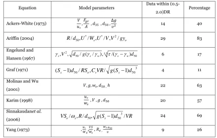
Table 1 illustrates the performance of nine sediment transport equations on Malaysian rivers, namely of Sungai Perak, Sungai Kemaman, Sungai Pergau and Sungai Kurau and the corresponding model parameters modified after Saleh et al. (2017). The nine equations used in analyses are Molinas and Wu (2001), Karim (1998), Yang (1973), Graf (1971) and Engelund and Hansen (1967). Table 2 shows the data range for d50 used in the analyses (Saleh 2016).

Table 1. Performance of nine sediment transport equations on Malaysian rivers and the corresponding model parameters (modified after Saleh et al., 2017)

Equation Model parameters Data within

(0.5-2.0)DR Percentage

Ackers-White (1973) 𝑉

𝑢∗,

𝐹𝑔𝑟

𝐴 , 𝑑35 , 𝑑50 , ∆𝑔

𝜐2 14 40

Ariffin (2004)

R

/

d

,

U

/

W

,

U

/

V

,

V

/

gy

Engelund and Hansen (1967)

5 . 1

50 50

2

)

/(

,

)

/

(

/

,

,

V

d

g

d

s















Graf (1971) 3

50 50

/

,

/

(

1

)

)

1

(

S



d

RS

C

VR

g

S



d

Molinas and Wu

(2001) 𝑉, 𝑔, 𝑤𝑠, 𝑑50 , ℎ 22 63

Karim (1998) 𝑢∗

𝑤𝑠

, 𝑉 , 𝑔 , 𝑑50 20 57

Sinnakaudanet al.

(2006)

VS

/

,

R

/

d

,

g

(

S

1

)

d

/

VR





Yang (1973) ,𝑢∗

𝑊𝑠, 𝑉𝑆 𝑊𝑠 , 𝑅𝑒 ,

𝑤_{𝑠 𝑑50}

3

Table 2. Total bed material load and data range for d50 (Saleh 2016)

Equation Data Range (mm)

Graf 0.09 < d50 < 2.78

Engelund and Hansen (E-H) 0.19 < d50 < 0.93

Yang 0.137 < d50 < 1.71

Ackers and White 0.04 < d50 < 4.94

Ariffin 0.37 < d50 < 4.00

Sinnakaudanetal. 0.3711< d50 < 4.00

III. DATA SELECTION

Data used in this study comprised of data from the works of Saleh et al. (2017), Department of Irrigation and Drainage (2013), Ibrahim (2012) and Ariffin (2004). There are 256 hydraulics, and sediment data measured from twelve rivers in Malaysia and the data range is given in Table 3.

A. Performance of Sediment Transport Equations on Twelve Rivers by

Various Investigators

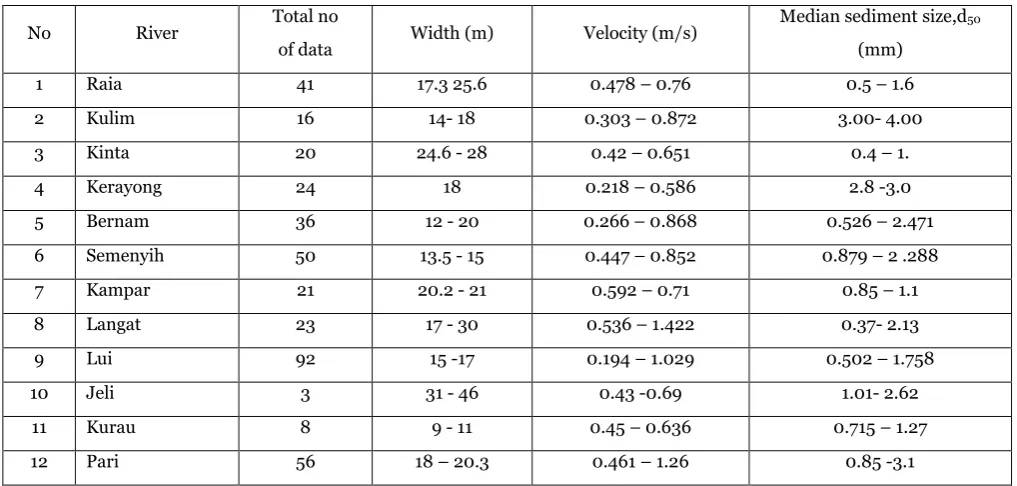
Table 4 shows the range of hydraulics and sediment data used in the analyses that include width, velocity and median size of sediment load. Table 5 illustrates the performance of selected equations on Malaysian river data.

Table 3. Data range used in analyses

Parameter Range

Total sediment load, Tj(kg/s) 0.0333-119.601

Flow, Q (m3_{/s) 0.737-87.792}

Velocity, V (m/s) 0.194-1.422

Depth of water, yo (m) 0.22-3.23

Particle mean size, d50 (mm) 0.37-4.9109

Water surface slope, So 0.0003-0.0167

Fall velocity, Ws(m/s) 0.043-21.157

Hydraulic radius, R (m) 0.21-2.66

Table 4. Range of hydraulics and sediment data used in analyses

No River Total no

of data Width (m) Velocity (m/s)

Median sediment size,d50 (mm)

1 Raia 41 17.3 25.6 0.478 – 0.76 0.5 – 1.6

2 Kulim 16 14- 18 0.303 – 0.872 3.00- 4.00

3 Kinta 20 24.6 - 28 0.42 – 0.651 0.4 – 1.

4 Kerayong 24 18 0.218 – 0.586 2.8 -3.0

5 Bernam 36 12 - 20 0.266 – 0.868 0.526 – 2.471

6 Semenyih 50 13.5 - 15 0.447 – 0.852 0.879 – 2 .288

7 Kampar 21 20.2 - 21 0.592 – 0.71 0.85 – 1.1

8 Langat 23 17 - 30 0.536 – 1.422 0.37- 2.13

9 Lui 92 15 -17 0.194 – 1.029 0.502 – 1.758

10 Jeli 3 31 - 46 0.43 -0.69 1.01- 2.62

11 Kurau 8 9 - 11 0.45 – 0.636 0.715 – 1.27

4

B. Robustness Measurement

The robustness measurement of all model parameters based on five parameter classes was derived from studies carried out by Ariffin (2017; 2004), Azamathulla et al. (2010), Sulaiman (2009), Sinnakaudan et al. (2006), and Chang et al. (2005). The variables are, relative roughness on the bed (R/d50) in flow resistance parameter class, stream-width ratio (B/yo) in conveyance and shape class which are shear velocity ratio to fall velocity (U*/s) and fall velocity to

shear velocity (s/U*), in sediment properties class is ratio of shear stress to average velocity (U*/V) and dimensionless unit stream power (VSo/s) in mobility class and the last variable is velocity head (v2_{/2g). The output variable} selected for this model is concentration by volume or

volumetric concentration (ratio of total sediment transport rate to flow rate) (Qt/Q).

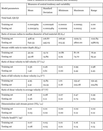
Data were randomly divided into two sets: a training set for model calibration and an independent validation set for model verification. In dividing the data into their sets, the training and testing sets were selected to be statistically consistent; thus, represent the same statistical population, as recommended by Shahin et al. (2004). In total, 174 data cases (68%) of the 256 data cases are used for training and balance 82 data cases (32%) for use for validation. The statistical analysis showing measures of central tendency (mean values) and variability (standard deviation, minimum and maximum values) is given in Table 6. Table 7 lists the model parameters used in the robustness analysis.

Table 5. Performance of selected equations on Malaysian river data

No. River Total No of data

Percentage of data within DR of 0.5 – 2.0

Engelund and Hansen

(1967)

Graf (1971) Ariffin (2004)

Chang et al.

(2005)

Sinnakaudan et al.

(2006)

1 Raia 41 0 0 61 63 66

2 Kulim 16 0 56 88 0 75

3 Kinta 20 20 30 45 0 30

4 Kerayong 24 21 50 83 0 58

5 Bernam 36 39 17 25 11 28

6 Semenyih 50 30 8 56 30 68

7 Kampar 21 38 0 0 28 48

8 Langat 23 17 0 43 13 57

9 Lui 92 14 2 46 22 63

10 Jeli 3 33 67 0 0 33

11 Kurau 8 0 0 0 38 88

5

Table 6. Measures of central tendency and variability

Model parameters

Measures of central tendency and variability

Mean Standard

Deviation Minimum Maximum Range

Total load, (Qt/Q)

Training set Testing set

0.0003569 0.0003974

0.0001926 0.0002484

0.00010 0.00009

0.00093 0.00215

0.00 0.00

Ratio of stream radius to median diameter of bed material (R/d50)

Training set Testing set

428.19 642.33

216.87 445.03

106.90 213.35

1229.73 2800.00

1122.84 2586.65

Stream width ratio to water depth (B/yo)

Training set Testing set

32.29 33.08

13.72 14.89

10.86 9.29

87.76 74.70

76.91 65.41

Ratio of shear velocity to fall velocity (U*/s)

Training set Testing set

0.56 1.40

0.26 0.61

0.01 0.00

0.99 5.44

0.98 5.43

Ratio of fall velocity to shear velocity (s/U*)

Training set Testing set

4.95 3.41

15.85 24.33

1.01 0.18

153.47 225.08

152.45 224.89

Ratio of shear velocity to average velocity (U*/V)

Training set Testing set

0.18 0.26

0.08 0.11

0.07 0.10

0.47 0.73

0.39 0.63

Dimensionless unit stream power (VS0/s)

Training set Testing set

0.01 0.03

0.01 0.02

0.00 0.00

0.02 0.12

0.02 0.12

Velocity head(V2_/_2g)

Training set Testing set

0.07 0.08

0.03 0.03

0.01 0.01

0.16 0.14

6

Table 7. Parameters used in robustness analysis

Name (R/d50) (B/yo) (U*/s) (s/U*) (U*/V) (VS0/s) (V2/2g)

Model1 / / / / / / /

Model2 / / / /

Model3 / / / / /

Model4 / / / / / /

Model5 / / / /

Model6 / / / / /

Model7 / / / / / /

Model8 / / / /

Model9 / / / / /

Model10 / / / / / /

Model11 / / / / /

Model12 / / / /

Model13 / / / / / /

Selection of the model parameters was carried out by trial-and-error approach in which a series of EPR models were trained using functions given in Table 8. A more detailed description of functions used for parameter selection can be found in the EPR Toolbox manual (Laucelli et al., 2009).

Table 8. Functions used for parameter selection Function Expression Structure f0 Y = sum(ai*X1*X2*f(X1)*f(X2))+ao

f1 Y = sum(ai*f(X1*X2))+ao

f2 Y = sum(ai*X1*X2*f(X1*X2))+ao LS Least square

LSN Non-negative least square

C. Model Approximations

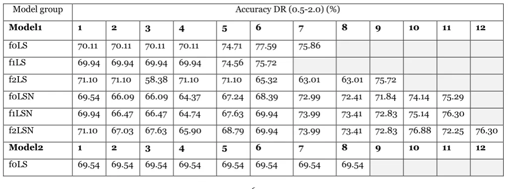
Models are approximated using Least Square (LS) and Non- Negative Least Square (LSN) methods. Accuracy of the models was measured using the discrepancy ratio of 0.5 – 2.0. Discrepancy ratio is the ratio of predicted to measured values. Performance of all models is shown in Table 9. Table 10 illustrates the best performing models of the model groups with the corresponding model exponential relations. The model parameters established from the robustness test are used as inputs in the EPR model. A total of 666 new models from 13 groups have been generated using 174 data in training set using the functions given in Table 8.

Table 9. Performance results of the EPR models during training

Model group Accuracy DR (0.5-2.0) (%)

Model1 1 2 3 4 5 6 7 8 9 10 11 12

f0LS 70.11 70.11 70.11 70.11 74.71 77.59 75.86 f1LS 69.94 69.94 69.94 69.94 74.56 75.72

f2LS 71.10 71.10 58.38 71.10 71.10 65.32 63.01 63.01 75.72

f0LSN 69.54 66.09 66.09 64.37 67.24 68.39 72.99 72.41 71.84 74.14 75.29 f1LSN 69.94 66.47 66.47 64.74 67.63 69.94 73.99 73.41 72.83 75.14 76.30 f2LSN 71.10 67.03 67.63 65.90 68.79 69.94 73.99 73.41 72.83 76.88 72.25 76.30

Model2 1 2 3 4 5 6 7 8 9 10 11 12

7

f1LS 69.94 69.94 69.94 69.94 69.94 69.94 69.94 69.94 f2LS 71.10 87.86 87.86 78.61 78.61 100.00 100.00

f0LSN 69.54 66.09 65.52 64.94 65.52 67.24 64.94 64.37 69.54 f1LSN 69.94 66.47 65.90 65.32 65.90 67.63 65.32 64.74 69.94 f2LSN 71.1 67.73 67.05 66.47 67.05 69.36 67.05

Model3 1 2 3 4 5 6 7 8 9 10 11 12

f0LS 70.11 86.78 86.78 77.01 77.01 98.28 90.23 f1LS 69.94 86.71 86.71 76.88 76.88 98.27 90.17

f2LS 71.10 71.10 71.10 71.10 71.10 71.10 71.10 71.10 71.10 f0LSN 69.54 66.09 65.52 64.94 65.52 67.24 65.52 64.94 70.11 f1LSN 69.94 66.47 65.90 65.32 65.90 69.36 66.47 65.90 71.86 f2LSN 71.10 67.63 67.05 66.47 67.05 69.36 67.05

Model4 1 2 3 4 5 6 7 8 9 10 11 12

f0LS 70.11 70.11 70.11 70.11 70.11 70.11

f1LS 69.94 69.94 69.94 69.94 69.94 69.94 69.94 65.90 f2LS 71.10 71.10 76.88 76.88 76.30 76.30 75.14 72.83

f0LSN 69.54 66.09 64.94 64.37 66.09 63.79 72.99 73.56 74.71 71.26 f1LSN 69.94 69.47 65.32 64.74 66.47 65.32 74.57 74.57 76.30 72.83 f2LSN 71.10 67.63 66.47 65.90 67.63 65.32 74.57 75.57 76.30 72.83

Model5 1 2 3 4 5 6 7 8 9 10 11 12

f0LS 61.49 86.78 77.01 77.01 f1LS

f2LS

f0LSN 60.92 66.09 66.67 67.82 67.24 67.82 68.39 68.39 f1LSN 61.27 66.47 67.05 68.21 67.63 69.36 69.36

f2LSN 67.63 68.21 68.21 68.79 69.36 69.36

Model6 1 2 3 4 5 6 7 8 9 10 11 12

f0LS 61.49 86.78 67.82 77.01 77.01 67.82 f1LS 61.27 86.71 67.63 76.88 76.88 67.63 f2LS 67.05 87.28 77.46 78.03 78.03

f0LSN 60.92 66.09 66.09 65.52 70.11 67.82 68.39 68.39 68.39 68.39 68.39

f1LSN 61.27 66.47 66.47 65.90 70.52 69.36 69.36 69.36 69.36 69.36

f2LSN 61.63 67.63 67.63 67.05 71.68 69.36 69.36 69.36

Model7 1 2 3 4 5 6 7 8 9 10 11 12

f0LS 67.24 0 68.39 64.37 70.11 70.11 70.11 70.11 f1LS 66.47 0 67.03 63.58 69.36 69.36 69.36 69.36 f2LS 67.63 67.63 69.36 65.32 67.63 67.63

f0LSN 66.67 66.09 66.67 72.99 72.99 69.54 66.67 71.26 70.69 68.39 f1LSN 67.05 66.47 67.05 73.41 71.10 71.10 67.63 72.25 71.68 69.36

f2LSN 67.63 67.63 68.21 67.05 69.05 69.36 69.36 76.30 73.41 73.99 74.57

8

f0LS 67.24 0 68.39 64.37 70.11 70.111 70.11 f1LS 67.05 0 68.21 64.16 69.94 69.94 69.94 f2LS 67.36 67.63 69.36 65.32 71.10 71.10 67.63 f0LSN 66.67 66.09 67.24 70.69 70.69 70.69

f1LSN 67.05 66.47 67.63 71.10 71.10 71.10 f2LSN 67.05 67.05 68.21 71.68 71.68 71.68

Model9 1 2 3 4 5 6 7 8 9 10 11 12

f0LS 67.24 86.78 0 66.09 66.09 66.67 66.67 66.67 66.67 f1LS 67.05 86.71 0 65.90 65.90 66.47 66.47 66.47 66.47 f2LS 67.63 67.63 67.63 67.63 67.63 67.63 67.63

f0LSN 66.67 66.09 67.24 70.69 70.69 68.97 68.97 f1LSN 67.05 66.47 67.63 71.10 71.10 70.52 69.94

f2LSN 67.63 67.63 68.79 72.25 72.25 70.52 68.79 69.94

Model10 1 2 3 4 5 6 7 8 9 10 11 12

f0LS 70.11 70.11 57.47 77.01 77.01 76.44 72.99 f1LS 69.94 69.94 57.23 76.88 76.88 76.30 72.83

f2LS 71.10 71.10 67.63 67.63 71.10 75.72 78.61 76.88

f0LSN 68.97 65.52 66.09 66.09 67.24 64.94 71.84 72.99 69.54 68.39 72.41 f1LSN 69.94 66.47 66.47 66.47 67.63 66.47 72.83 73.99 70.52 69.36 73.99 f2LSN 71.10 67.63 67.63 65.90 68.79 66.47 73.99 73.41 72.83 72.25 70.52

Model11 1 2 3 4 5 6 7 8 9 10 11 12

f0LS 70.11 70.11 70.11 70.11 70.11 70.11 66.09 64.94 f1LS 69.94 69.94 69.94 69.94 69.94 69.94 65.90 67.40 f2LS 71.10 87.86 87.86 100.00 60.12 73.99

f0LSN 69.54 66.09 64.94 64.37 66.09 63.79 72.99 73.56 74.71 f1LSN 69.54 66.47 65.32 64.74 66.47 65.32 74.57 74.57 76.30 f2LSN 70.52 67.05 65.90 65.32 67.05 74.57 73.99 73.99 75.72

Model12 1 2 3 4 5 6 7 8 9 10 11 12

f0LS 62.43 87.86 68.79 78.61 78.61 72.25 69.36 71.86 68.21 67.63 f1LS 62.43 87.86 68.79 78.61 78.61 72.25 69.36 71.86 68.21 f2LS 67.63 87.86 78.03 78.61 78.61 76.72 75.14

f0LSN 60.92 65.52 65.52 65.52 70.11 67.82 68.39 f1LSN 61.27 65.90 65.90 65.90 70.52 69.36 69.36

f2LSN 67.63 67.63 67.63 68.21 67.05 67.63 67.63 67.05

Model13 1 2 3 4 5 6 7 8 9 10 11 12

f0LS 71.10 87.86 0 0 78.61 77.46 73.99 80.35 80.35 80.35 71.10 f1LS 71.10 87.86 0 0 78.61 77.46 73.99 80.35 80.35 80.35 71.10

f2LS 71.10 71.10 67.63 67.63 71.10 65.32 64.74 63.58 75.72 67.63 67.63 60.21 f0LSN 69.54 66.09 64.94 68.97 68.97 67.21 71.84 71.26 68.97 68.39 71.84

9

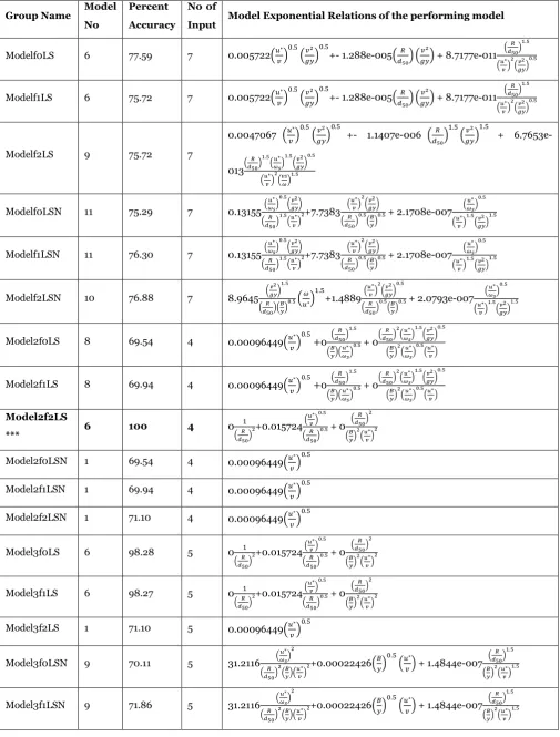
Table 10. Model Exponential Relations of the performing model

Group Name Model

No

Percent

Accuracy

No of

Input Model Exponential Relations of the performing model

Modelf0LS 6 77.59 7 0.005722(𝑢∗

𝑣) 0.5

(𝑣2

𝑔𝑦) 0.5

+- 1.288e-005(𝑅

𝑑50) (

𝑣2

𝑔𝑦) + 8.7177e-011 (𝑅 𝑑50) 1.5 (𝑢∗ 𝑣) 2 (𝑣2 𝑔𝑦) 0.5

Modelf1LS 6 75.72 7 0.005722(𝑢∗

𝑣) 0.5

(𝑣2

𝑔𝑦) 0.5

+- 1.288e-005(𝑅

𝑑50) (

𝑣2

𝑔𝑦) + 8.7177e-011 (𝑅 𝑑50) 1.5 (𝑢∗ 𝑣) 2 (𝑣2 𝑔𝑦) 0.5

Modelf2LS 9 75.72 7

0.0047067 (𝑢∗

𝑣) 0.5

(𝑣2

𝑔𝑦) 0.5

+- 1.1407e-006 (𝑅

𝑑50)

1.5

(𝑣2

𝑔𝑦) 1.5

+

6.7653e-013( 𝑅 𝑑50) 1.5 (𝑢∗_𝜔𝑠) 1.5

(𝑣2_𝑔𝑦)

0.5 (𝑢∗ 𝑣) 2 (𝑣𝑠 𝜔) 1.5

Modelf0LSN 11 75.29 7 0.13155(

𝑢∗ 𝜔𝑠)

0.5

(𝑣2

𝑔𝑦)

(_𝑑50𝑅)1.5(𝑢∗_𝑣)2

+7.7383 ( 𝑢∗ 𝑣) 2 (𝑣2 𝑔𝑦) (𝑅 𝑑50) 0.5 (𝐵 𝑦)

0.5 + 2.1708e-007

(_𝜔𝑠𝑢∗) 0.5 (𝑢∗ 𝑣) 1.5 (𝑣2 𝑔𝑦) 1.5

Modelf1LSN 11 76.30 7 0.13155(

𝑢∗ 𝜔𝑠)

0.5

(𝑣2_𝑔𝑦) (𝑅 𝑑50) 1.5 (𝑢∗ 𝑣) 2+7.7383 (𝑢∗_𝑣) 2

(𝑣2_𝑔𝑦) (𝑅

𝑑50) 0.5

(𝐵

𝑦)

0.5 + 2.1708e-007

(𝑢∗ 𝜔𝑠) 0.5 (𝑢∗ 𝑣) 1.5 (𝑣2 𝑔𝑦) 1.5

Modelf2LSN 10 76.88 7 8.9645 (

𝑣2 𝑔𝑦) 1.5 (𝑅 𝑑50)( 𝐵 𝑦) 0.5( 𝜔 𝑢∗) 1.5 +1.4889( 𝑢∗ 𝑣) 2

(_𝑔𝑦𝑣2)

0.5 (𝑅 𝑑50) 0.5 (𝐵 𝑦)

0.5 + 2.0793e-007

(𝑢∗ 𝜔𝑠) 0.5 (𝑢∗ 𝑣) 1.5 (𝑣2 𝑔𝑦) 1.5

Model2f0LS 8 69.54 4 0.00096449(𝑢∗

𝑣) 0.5

+0 (

𝑅 𝑑50)

1.5

(𝐵_𝑦)(𝑢∗_𝜔𝑠)0.5 + 0(

𝑅 𝑑50) 2 (𝑢∗ 𝜔𝑠) 1.5 (𝑣2 𝑔𝑦) 0.5

(𝐵_𝑦)2(𝑢∗_𝜔𝑠)0.5(𝑢∗_𝑣)

Model2f1LS 8 69.94 4 0.00096449(𝑢∗

𝑣) 0.5

+0 (

𝑅 𝑑50) 1.5 (𝐵 𝑦)( 𝑢∗ 𝜔𝑠)

0.5 + 0

(𝑅 𝑑50) 2 (𝑢∗ 𝜔𝑠) 1.5 (𝑣2 𝑔𝑦) 0.5 (𝐵 𝑦) 2 (𝑢∗ 𝜔𝑠) 0.5 (𝑢∗ 𝑣) Model2f2LS

*** 6 100 4 0

1 (_𝑑50𝑅)2

+0.015724( 𝑢∗ 𝑣) 0.5 (𝑅 𝑑50) 0.5 + 0

(𝑅 𝑑50) 2 (𝐵 𝑦) 2 (𝑢∗ 𝑣) 2

Model2f0LSN 1 69.54 4 0.00096449(𝑢∗

𝑣) 0.5

Model2f1LSN 1 69.94 4 0.00096449(𝑢∗

𝑣) 0.5

Model2f2LSN 1 71.10 4 0.00096449(𝑢∗

𝑣) 0.5

Model3f0LS 6 98.28 5 0 1

(𝑅 𝑑50) 2+0.015724 (𝑢∗ 𝑣) 0.5

(_𝑑50𝑅)0.5 + 0 (

𝑅 𝑑50) 2 (𝐵 𝑦) 2 (𝑢∗ 𝑣) 2

Model3f1LS 6 98.27 5 0 1

(𝑅 𝑑50) 2+0.015724 (𝑢∗ 𝑣) 0.5 (𝑅 𝑑50) 0.5 + 0

(_𝑑50𝑅)2 (𝐵 𝑦) 2 (𝑢∗ 𝑣) 2

Model3f2LS 1 71.10 5 0.00096449(𝑢∗

𝑣) 0.5

Model3f0LSN 9 70.11 5 31.2116 (

𝑢∗ 𝜔𝑠) 2 (𝑅 𝑑50) 2 (𝐵 𝑦)( 𝑢∗ 𝑣)

2+0.00022426(

𝐵 𝑦)

0.5

(𝑢∗

𝑣) + 1.4844e-007 (𝑅

𝑑50) 1.5

(𝐵_𝑦)2(𝑢∗_𝑣)1.5

Model3f1LSN 9 71.86 5 31.2116 (

𝑢∗ 𝜔𝑠)

2

(_𝑑50𝑅)2(𝐵_𝑦)(𝑢∗_𝑣)2

+0.00022426(𝐵

𝑦) 0.5

(𝑢∗

𝑣) + 1.4844e-007 (𝑅

𝑑50) 1.5

10 Model3f2LSN 1 71.10 5 0.00096449(𝑢∗

𝑣) 0.5

Model4f0LS 1 70.11 6 0.00096449(𝑢_𝑣∗)0.5

Model4f1LS 1 69.94 6 0.00096449(𝑢∗

𝑣) 0.5

Model4f2LS 3 76.88 6 +-0.00011109 1

(_𝑢∗𝜔)1.5(𝑢∗_𝑣)1.5

+0.0010153 1 (𝜔

𝑢∗) 0.5

Model4f0LSN 9 74.71 6 18.7575(

𝑣𝑠 𝜔) 0.5 (𝑅 𝑑50)( 𝐵 𝑦)

+ 1.3436e-007 1 (𝐵_𝑦)(_𝑢∗𝜔)2(𝑢∗_𝑣)1.5(𝑣𝑠_𝜔)1.5

+ 0.00018294(𝐵

𝑦) 0.5

(𝑢∗

𝑣)

Model4f1LSN 9 76.30 6 18.7575(

𝑣𝑠 𝜔) 0.5 (𝑅 𝑑50)( 𝐵 𝑦)

+ 1.3436e-007 1 (𝐵 𝑦)( 𝜔 𝑢∗) 2 (𝑢∗ 𝑣) 1.5 (𝑣𝑠 𝜔)

1.5+ 0.00018294(

𝐵 𝑦)

0.5

(𝑢_𝑣∗)

Model4f2LSN 9 76.30 6 18.7575(

𝑣𝑠 𝜔) 0.5 (𝑅 𝑑50)( 𝐵 𝑦)

+ 1.3436e-007 (

𝑢∗ 𝜔𝑠) 2 (𝐵 𝑦)( 𝑢∗ 𝑣) 1.5 (𝑣𝑠 𝜔)

1.5+ 0.00018294(

𝐵 𝑦)

0.5

(𝑢∗

𝑣)

Model5f0LS 2 86.78 4 0.00041211(𝑢∗

𝜔𝑠)

0.5

(𝜔

𝑢∗)

0.5

Model5f1LS - - - -

Model5f2LS - - - -

Model5f0LSN 7 68.39 4 3936.6496 (

𝑢∗ 𝜔𝑠) 2 (𝑅 𝑑50) 2 (𝐵 𝑦)

1.5+ 0.0003356 (

𝑢∗ 𝜔𝑠) 0.5 (𝜔 𝑢∗) 0.5

+ 1.5921e-005(

𝑅 𝑑50)

(𝐵

𝑦) 2

Model5f1LSN 6 69.36 4 3986.4618 (

𝑢∗ 𝜔𝑠) 2 (𝑅 𝑑50) 2 (𝐵 𝑦)

1.5+ 0.0029567

1 (𝐵

𝑦)

2+ 0.00034401(

𝑢∗

𝜔𝑠)

0.5

(_𝑢𝜔∗)

0.5

Model5f2LSN 5 69.36 4 3986.4618 (

𝑢∗ 𝜔𝑠) 2 (𝑅 𝑑50) 2 (𝐵 𝑦)

1.5+ 0.0029567

1 (𝐵_𝑦)2+

0.000344011 (𝐵

𝑦)

Model6f0LS 2 86.78 5 0₍𝑅1

𝑑50)

1.5 + 0.006834

1 (𝑅

𝑑50) 0.5

Model6f1LS 2 86.71 5 0₍𝑅1

𝑑50)

1.5 + 0.006834

1 (_𝑑50𝑅)0.5

Model6f2LS 2 87.28 5 0₍𝑅1

𝑑50)

1.5 + 0.006834

1 (𝑅

𝑑50) 0.5

Model6f0LSN 5 70.11 5 0.31667 (

𝑣𝑠 𝜔)

(_𝑑50𝑅)0.5(_𝜔𝑠𝑢∗)

+ 2.461e-007 1 (𝑣𝑠_𝜔)2(𝑣𝑠_𝜔)1.5

Model6f1LSN 5 70.52 5 0.31667 (

𝑣𝑠 𝜔) (𝑅 𝑑50) 0.5 (𝑢∗ 𝜔𝑠)

+ 2.461e-007 1 (𝑣𝑠 𝜔) 2 (𝑣𝑠 𝜔) 1.5

Model6f2LSN 5 71.68 5 0.31667(

𝜔 𝑢∗)(

𝑣𝑠 𝜔)

(_𝑑50𝑅)0.5

+ 2.461e-007(

𝑢∗ 𝜔𝑠)

2

(𝑣𝑠_𝜔)1.5

Model7f0LS 5 70.11 6 0(𝜔

𝑢∗)

0.5

+ 0.0022795(𝑅

𝑑50)

0.5

(𝑣2

𝑔𝑦) 0.5

+ −2.622𝑒 − 005 (𝑅

𝑑50) (

𝑣2

𝑔𝑦)

Model7f1LS 5 69.36 6 0(𝜔

𝑢∗)

0.5

+ 0.0022795(𝑅

𝑑50)

0.5

(𝑣2

𝑔𝑦) 0.5

+ −2.622𝑒 − 005 (𝑅

𝑑50) (

𝑣2

𝑔𝑦) Model7f2LS 3 69.36 6 3.36883e-005(_𝑑𝑅

50)

0.5

+ −4.3848𝑒 − 005 (_𝑑𝑅

50)

1.5

11

Model7f0LSN 4 72.99 6 20.2894(

𝑣𝑠 𝜔) 0.5 (𝑅 𝑑50)( 𝐵 𝑦)

+ 6.2504e-005 1 (𝑣2

𝑔𝑦) 0.5

Model7f1LSN 4 73.41 6 20.2894(

𝑣𝑠 𝜔) 0.5 (𝑅 𝑑50)( 𝐵 𝑦)

+ 6.2504e-005 1 (𝑣2

𝑔𝑦) 0.5

Model7f2LSN 8 76.30 6 0.54817 (

𝜔 𝑢∗)( 𝑣𝑠 𝜔) (𝑅 𝑑50) 0.5 (𝐵 𝑦) 0.5 (𝑣2 𝑔𝑦)

0.5+ 1.8413e-007

1

(_𝑢∗𝜔)2(𝑣𝑠_𝜔)1.5+ 0.00029659 ( 𝑣𝑠 𝜔)

0.5

Model8f0LS 5 70.11 4 0 1

(𝑢∗

𝜔𝑠)

0.5+ −0.00022795 (

𝑅 𝑑50)

0.5

(𝑣2

𝑔𝑦) 0.5

+ −2.622𝑒 − 005 (𝑅

𝑑50) (

𝑣2

𝑔𝑦)

Model8f1LS 5 69.94 4 0 1

(𝑢∗

𝜔𝑠)

0.5+ −0.00022795 (

𝑅 𝑑50)

0.5

(_𝑔𝑦𝑣2)0.5+ −2.622𝑒 − 005 (_𝑑𝑅

50) (

𝑣2

𝑔𝑦)

Model8f2LS 5 71.10 4 0(𝑣2

𝑔𝑦) + 3.1645𝑒 − 005 ( 𝑅 𝑑50)

0.5

+ −9.0277𝑒 − 006 (𝑅

𝑑50) (

𝑣2

𝑔𝑦)

Model8f0LSN 4 70.69 4 8.3922 (

𝑣2 𝑔𝑦) 1.5 (𝑅 𝑑50)( 𝐵 𝑦)

0.5+ 7.6601e-005

1 (𝑣2

𝑔𝑦) 0.5

Model8f1LSN 4 71.10 4 8.3922 (

𝑣2 𝑔𝑦)

1.5

(_𝑑50𝑅)(𝐵_𝑦)0.5

+ 7.6601e-005 1 (𝑣2

𝑔𝑦) 0.5

Model8f2LSN 4 71.68 4 8.3922 (

𝑣2 𝑔𝑦)

1.5

(_𝑑50𝑅)(𝐵_𝑦)0.5

+ 7.6601e-005 1 (𝑣2

𝑔𝑦) 0.5

Model9f0LS 2 86.78 5 0₍𝑅1

𝑑50)

1.5+ 0.0068341

1 (𝑅

𝑑50) 0.5

Model9f1LS 2 86.71 5 0₍𝑅1

𝑑50)

1.5+ 0.0068341

1 (𝑅

𝑑50) 0.5

Model9f2LS 1 67.63 5 0.00041211(𝐵

𝑦) 0.5

Model9f0LSN 4 70.69 5 8.3922 (

𝑣2 𝑔𝑦) 1.5 (𝑅 𝑑50)( 𝐵 𝑦)

0.5+ 7.6601e-005

1 (𝑣2

𝑔𝑦) 0.5

Model9f1LSN 4 71.10 5 8.3922 (

𝑣2 𝑔𝑦)

1.5

(_𝑑50𝑅)(𝐵_𝑦)0.5

+ 7.6601e-005 1 (𝑣2

𝑔𝑦) 0.5

Model9f2LSN 4 72.25 5 8.3922 (

𝑣2 𝑔𝑦) 1.5 (𝑅 𝑑50)( 𝐵 𝑦)

0.5+ 7.6601e-005

1 (𝑣2

𝑔𝑦) 0.5

Model10f0LS 4 77.01 6 2.8718₍𝑅1 𝑑50)

1.5+ 0.31095

1 (𝑅

𝑑50)

+ 0 1 (𝑢∗ 𝜔𝑠) 1.5 (𝑣2 𝑔𝑦) 2

Model10f1LS 4 76.88 6 2.8718₍𝑅1 𝑑50)

1.5+ 0.31095

1 (_𝑑50𝑅) + 0

1 (_𝜔𝑠𝑢∗)1.5(𝑣2_𝑔𝑦)

2

Model10f2LS 7 78.61 6

0 . 005722 (𝑢∗

𝑣) 0.5

(𝑣2

𝑔𝑦) 0.5

+ −1.288𝑒 − 005 (𝑅

𝑑50) (

𝑣2

𝑔𝑦) + 8.7177𝑒 −

011 ( 𝑅 𝑑50) 1.5 (𝑢∗ 𝑣) 2 (𝑣2 𝑔𝑦) 0.5

Model10f0LSN 8 72.99 6 0.10676(

𝑢∗ 𝑣)(

𝑣2 𝑔𝑦)

0.5

(_𝑑50𝑅)0.5

+ 3.9855e-007 (

𝑢∗ 𝜔𝑠)

(𝐵_𝑦)0.5(𝑢∗_𝑣)2(_𝑔𝑦𝑣2)

1.5+ 0.00016018 (

𝑢∗

12

Model10f1LSN 8 73.99 6 0.10676(

𝑢∗ 𝑣)( 𝑣2 𝑔𝑦) 0.5 (𝑅 𝑑50)

0.5 + 3.9855e-007

(𝑢∗ 𝜔𝑠) (𝐵 𝑦) 0.5 (𝑢∗ 𝑣) 2 (𝑣2 𝑔𝑦)

1.5+ 0.00016018 (

𝑢∗

𝑣) 1.5

Model10f2LSN 7 73.99 6 4.6159 (

𝑢∗ 𝑣)

1.5

(𝑣2

𝑔𝑦)

(_𝑑50𝑅)0.5(𝐵_𝑦)0.5

+ 2.1553e-007 (

𝑢∗ 𝜔𝑠) 0.5 (𝑢∗ 𝑣) 1.5 (𝑣2 𝑔𝑦) 1.5

Model11f0LS 1 70.11 5 0.00096449(𝑢∗

𝑣) 0.5

Model11f1LS 1 69.94 5 0.00096449(𝑢∗

𝑣) 0.5

Model11f2LS

*** 4 100.00 5 0

1 (𝑅 𝑑50) 2+0.015724 (𝑢∗ 𝑣) 0.5

(_𝑑50𝑅)0.5 + 0 1

(𝑢∗

𝑣) 1.5

Model11f0LSN 9 74.71 5 18.7575(

𝑣𝑠 𝜔) 0.5 (𝑅 𝑑50)( 𝐵 𝑦)

+ 1.3436e-007 (

𝑢∗ 𝜔𝑠)

2

(𝐵_𝑦)(𝑢∗_𝑣)1.5(𝑣𝑠_𝜔)1.5

+ 0.00018294(𝐵

𝑦) 0.5

(𝑢∗

𝑣)

Model11f1LSN 9 76.30 5 18.7575(

𝑣𝑠 𝜔) 0.5 (𝑅 𝑑50)( 𝐵 𝑦)

+ 1.3436e-007 (

𝑢∗ 𝜔𝑠) 2 (𝐵 𝑦)( 𝑢∗ 𝑣) 1.5 (𝑣𝑠 𝜔)

1.5+ 0.00018294(

𝐵 𝑦)

0.5

(𝑢∗

𝑣)

Model11f2LSN 6 74.57 5 20.6487(

𝑣𝑠 𝜔) 0.5 (𝑅 𝑑50)( 𝐵 𝑦)

+ 0.00078901(𝑢∗

𝑣) + 1.4956e-007 (𝑢∗ 𝜔𝑠) 2 (𝑣𝑠 𝜔) 1.5

Model12f0LS 2 87.86 4 0₍𝑅1

𝑑50)

1.5+ 0.0068341

1 (𝑅

𝑑50) 0.5

Model12f1LS 2 87.86 4 0₍𝑅1

𝑑50)

1.5+ 0.0068341

1 (𝑅

𝑑50) 0.5

Model12f2LS 2 87.86 4 0₍𝑅1

𝑑50)

1.5+ 0.0068341

1 (_𝑑50𝑅)0.5

Model12f0LSN 5 70.11 4 0.31667 (

𝑣𝑠 𝜔) (𝑅 𝑑50) 0.5 (𝑢∗ 𝜔𝑠)

+ 2.461e-007(

𝑢∗ 𝜔𝑠) 2 (𝑣𝑠 𝜔) 1.5

Model12f1LSN 5 70.52 4 0.31667 (

𝑣𝑠 𝜔)

(_𝑑50𝑅)0.5(_𝜔𝑠𝑢∗)

+ 2.461e-007(

𝑢∗ 𝜔𝑠)

2

(𝑣𝑠_𝜔)1.5

Model12f2LSN 4 68.21 4 0.12605(

𝑣𝑠 𝜔)

1.5

(𝑢∗

𝜔𝑠)

1.5+ 2.7393e-007

(𝑢∗_𝜔𝑠)

2

(𝑣𝑠

𝜔) 1.5

Model13f0LS 2 87.86 6 0₍𝑅1

𝑑50)

1.5+ 0.0068341

1 (_𝑑50𝑅)0.5

Model13f1LS 2 87.86 6 0₍𝑅1

𝑑50)

1.5+ 0.0068341

1 (𝑅

𝑑50) 0.5

Model13f2LS 9 75.72 6

0 . 00471 (𝑢∗

𝑣) 0.5

(𝑣2

𝑔𝑦) 0.5

+ −1.1512𝑒 − 006 (𝑅

𝑑50)

1.5

(𝑣2

𝑔𝑦) 1.5

+ 7.157𝑒 −

013( 𝑅 𝑑50) 1.5 (𝑢∗ 𝜔𝑠)( 𝑣2 𝑔𝑦) 2 (𝑢∗ 𝑣) 1.5 (𝑣𝑠 𝜔) 2

Model13f0LSN 7 71.84 6 15.2937 (

𝑣2 𝑔𝑦) (𝑅 𝑑50)( 𝐵 𝑦)

+ 0.0077026(𝑢∗

𝑣) 1.5

(𝑣2

𝑔𝑦) 0.5

+ 2.0303e-007(

𝑢∗ 𝜔𝑠) 2 (𝑣𝑠 𝜔) 1.5

Model13f1LSN 7 72.83 6 15.2937 (

𝑣2 𝑔𝑦)

(_𝑑50𝑅)(𝐵_𝑦)+ 0.0077026( 𝑢∗

𝑣) 1.5

(𝑣2

𝑔𝑦) 0.5

+ 2.0303e-007(

13

Model13f2LSN 6 73.99 6 4.5415(

𝑢∗ 𝑣)

1.5

(𝑣2

𝑔𝑦)

(𝑅

𝑑50) 0.5

(𝐵

𝑦)

0.5+ 2.4772e-007

(𝑢∗_𝜔𝑠)

2

(𝑣𝑠

𝜔) 1.5

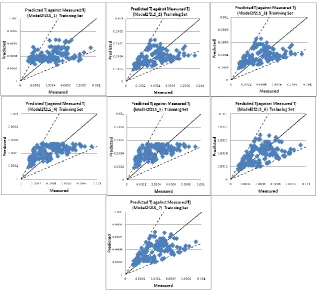
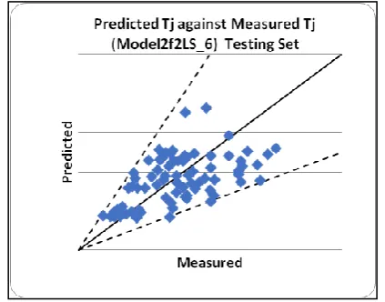
14 Figure 1 shows performance of Group Model2f2LS (Model 1 until Model 7). Seven newly developed models have shown

to predict the measured values within an acceptable limit. The model that best predicts the measured values is Model 6.

Figure 1. Model performance for Group Model2f2LS (Model 1 until Model 7)

Models in Figure 2 exhibit similar trends to Figure 1. Analyses suggest that Model 4 exhibit the best predictions compare to other 5 models.

Figure 2. Model performance Group Model11f2LS (Model 1 until Model 6)

Results with data confirmation from Table 10 suggest that Model 6 (Model2f2LS) yield 100 percent accuracy in prediction. The exponential relations of Model 6

15 Model 6 (Model2f2LS)

𝑄𝑡

𝑄 = 0

1

(𝑅 𝑑50)

2+0.015724 (𝑢∗

𝑣) 0.5

( 𝑅 𝑑50)

0.5 + 0 ( 𝑅

𝑑50) 2

(𝐵_𝑦)2(𝑢∗_𝑣)

2 (1)

Model 4 (Model 11f2LS)

𝑄𝑡

𝑄 = 0

1

( 𝑅 𝑑50)

2+0.015724 (𝑢∗

𝑣) 0.5

( 𝑅 𝑑50)

0.5 + 0 1

(𝑢∗_𝑣)

1.5 (2)

Both models 6 and 4 (Equations 1 and 2) suggest 𝑈∗

𝑉 (ratio of shear velocity to flow velocity) and 𝑅

𝑑50

(ratio of hydraulic

radius to mean sediment diameter) as the most significant and influential parameters. With the above discovery, the general expression for sediment concentration can be expressed as follows;

𝑄𝑡

𝑄 = 0.015724

(𝑈∗⁄ )_𝑉0.5 (𝑅 𝑑⁄50)

0.5 (3)

where; Qt is sediment total load (kg/s); V is flow velocity (m/s), d50 is median diameter of sediment load (m), Q is flow discharge (kg/s), U * is shear velocity (m/s) and R is hydraulic radius (m).

Figure 3. Graph of measured sediment total load versus predicted sediment total load using 82 testing data

IV. CONCLUSION

Analyses carried out on the model parameters have

indicated that two variables namely 𝑈∗

𝑉 (ratio of shear velocity to flow velocity) and 𝑅

𝑑50

(ratio of hydraulic radius to

mean sediment diameter) to be the most significant and influential parameters. The above is confirmed by the performance of the model with 100 percent prediction accuracy. This new model is an improved model of Ariffin (2004), of which the latter has used four model parameters as predictors. In the improved model, analyses have confirmed that only two parameters could predict with greater accuracy the measured sediment load values.

V. ACKNOWLEDGEMENT

16

VI. REFERENCES

[1] Ackers, P & White, WR 1973, ‘Sediment transport: New approach and analysis’, Journal of the Hydraulics Division, vol. 99, no. 11, pp. 2041– 2060.

[2]Ariffin, J 2004, ‘Development of sediment transport models for rivers in Malaysia using regression analysis and artificial neural networks’, PhD thesis, Universiti Sains Malaysia, Penang, Malaysia.

[3]Ariffin, J 2017, Fluvial geomorphology anthropogenic agents of change and their

implications, Penerbit Press Universiti Teknologi MARA, Malaysia.

[4]Azamathulla, HM, Ab Ghani, A, Zakaria, NA & Chang, CK, Abu Hasan, Z 2010, ‘Genetic programming approach to predict sediment concentration for Malaysia rivers’, International Journal of Ecological Economics and Statistics, vol. 16, no. 10, pp. 53–64.

[5]Chang, CK, Ab Ghani, A, Zakaria, NA, Abu Hasan, Z & Abdullah, R 2005, ‘Sediment transport equation assessment for selected rivers in Malaysia’, International Journal of River Basin Management, vol. 3, no. 3, pp. 203–208.

[6]Department of Irrigation and Drainage 2009,

River sand mining management guideline,

Department of Irrigation and Drainage, Kuala Lumpur.

[7]Department of Irrigation and Drainage 2013,

Kajian pengumpulan data dan analisis Endapan

Sungai, Final report vol. 1, pp. 49–56.

[8]Doglioni, A & Simeone, V 2017, ‘Evolutionary modelling of response of water table to precipitations’, Journal of Hydrologic Engineering, vol. 22, no. 2, pp. 04016055. [9]Draper, NR & Smith, H 1998, Applied regression

analysis, John Wiley and Sons, New York.

[10] Engelund, F & Hansen, E 1967, A monograph on sediment transport in alluvial streams, Teknisk Forlag, Copenhagen.

[11] Ghorbani, A & Hasanzadehshooiili, H 2018, ‘Prediction of UCS and CBR of microsilica-lime stabilized sulphate silty sand using ANN and EPR Models; application to the deep soil mixing’,

Journal Soils and Foundations, vol. 58, no. 1, pp. 34–49.

[12] Giustolisi, O & Savic, DA 2006, ‘A symbolic data driven technique based on evolutionary polynomial regression’, Journal of Hydroinformatics, vol. 8, no. 3, pp. 207–222.

[13] Giustolisi, O, Doglioni, A, Savic, DA & di Pierro, F 2008, ‘An evolutionary multiobjective strategy for the effective management of groundwater resources’, Water Resources Research Journal, vol. 44, no. 1, pp. 1–14.

[14] Graf, WH & Acaroglu, ER 1968, ‘Sediment transport in conveyances systems, Part 1’,

International Association of Scientific Hydrology, vol. 13, no. 2, pp. 20–39.

[15] Ibrahim, NA 2012, ‘Penilaian dan Pembangunan Persamaan Pengangkutan Endapan Sungai-Sungai di Malaysia’, Final thesis, Universiti Sains Malaysia, Penang, Malaysia.

[16] Karim, F 1998, ‘Bed Material discharge prediction for non-uniform bed sediments’, Hydraulic Engineering, vol. 124, no. 6, 597–604.

[17] Koza, JR 1992, Genetic programming: On the programming of computers by means of natural

selection, A Bradford Book, The MIT Press,

Massachusetts, London, England.

[18] Laucelli, D, Berardi, L & Dogliono, A 2009,

Evolutionary Polynomial Regression (EPR)

Toolbox, Version 2.0SA (Stand Alone Version), Department of Civil and Environmental Engineering, Technical University of Bari, Italy. [19] Molinas, A & Wu, B 2001, ‘Transport of Sediment

in Large Sand-bed Rivers’, Journal of Hydraulic Research, vol. 39, no. 2, pp. 135–146.

17 Malaysia, Penang, Malaysia.

[21] Saleh, A, Abustan, I, Mohd Remy Rozainy, MAZ & Sabtu, N 2017, ‘Assessment of total bed material equations on selected Malaysia rivers’, in AIP Conference Proceeding, vol. 1892, no. 1, pp. 070002.

[22] Savic, DA, Giutolisi, O, Berardi, L, Shepherd, W, Djordjevic, S & Saul, A 2006, ‘Modelling sewer failure by evolutionary computing’, in Proceeding of the Institution of Civil Engineers, Water

Management, vol. 159, no. 2, pp. 111–118.

[23] Shahin, MA, Maier, HR & Jaksa, MB 2004, ‘data division for developing neural networks applied to geotechnical engineering’, Journal of Computing in Civil Engineering, ASCE, vol. 18, no. 2, pp. 105– 114.

[24] Sinnakaudan, SK, Ab Ghani, A, Ahmad, MS & Zakaria, NA 2006, ‘Multiple linear regression model for total bed material load prediction’,

Journal of Hydraulic Engineering, vol. 132, no. 5, pp. 521–528.

[25] Sulaiman, MS 2009, ‘Sediment transport equation development for highland rivers in Malaysia’, Master’s thesis, Universiti Teknologi MARA, Malaysia.

[26] Yang, C.T 1973, ‘Incipient Motion and Sediment Transport’, Journal of the Hydraulics Division, vol. 99, no. 10, pp. 1679–1704.