United Kingdom Vol. IV, Issue 10, October 2016
Licensed under Creative Common Page 159
http://ijecm.co.uk/
ISSN 2348 0386
DETERMINANTS OF KENYA’S BILATERAL TRADE FLOWS
Joy Waithira Ngugi
Department of Economics, Accounting and Finance, School of Business, Jomo Kenyatta University of Agriculture and Technology, Kenya
joywngugi@gmail.com
Abstract
The purpose of this study was to identify the factors that determine Kenya’s bilateral trade flows
using the gravity model approach. The specific objective of the study was to evaluate the effect
of institutional quality, regional trade agreements, internal transport infrastructure, gross
domestic product and distance on Kenya’s bilateral trade flows. The study examined total trade
flows between Kenya and five of its trading partners in East Africa over the sample period
1994-2014. The study employed judgmental sampling technique in selecting Kenya’s trading partners
from a larger population where large trade volumes between countries indicated a key trading
partner and small trade volumes indicated otherwise. It employed the ordinary least squares
method and the random effects method to estimate the augmented gravity model equation. The
study findings indicated that; Kenya’s total trade flows are positively and significantly determined
by its own gross domestic productand that of its trading partner, and diminish significantly with
geographical distance between Kenya and its trading partner. The study also revealed that
internal transport infrastructure and institutional quality exert a positive and significant influence
on Kenya’s trade flows. Membership to the East African Community was found to have a
negative and statistically insignificant effect on bilateral trade. The findings accentuate the
urgent need to radically expand, improve and modernize trade-related infrastructure in Kenya.
In addition, policies and legislative reforms aimed at promoting transparency, accountability and
integrity in our institutions should be pursued. Lastly, in order to deepen the degree of
integration and increase intra-regional trade flows, there is an urgent need for the removal of
trade barriers at the various borders of the member states of the East African Community.
Keywords: Bilateral trade, gravity model, East African Community, institutional quality,
Licensed under Creative Common Page 160 INTRODUCTION
Foreign trade is understood as a country‟s trade with other countries. It is the exchange of capital, goods, and services across international borders or territories. Bilateral trade is a form of foreign trade and refers to a system of trading between two countries in which each country attempts to balance its trade with that of the other. A nation‟s trade with others consists of imports and exports flowing in and out of the country respectively. International trade arises because no country can be completely self-sufficient. Trade between countries is therefore essential to ensure the supply of a country‟s goods and services. There is unequal distribution of productive resources by the nature on the surface of the earth. Countries differ in respect of climatic conditions, availability of cultivable land, forests, mineral products, labor, capital, technology, and entrepreneurial skills. Given the diversities of resource endowment, no country has the potential to produce all the commodities at the least cost. Through international trade nations are able to specialize in those goods they can produce most cheaply and efficiently. They export such products to others and in turn import those products in which they have comparative cost disadvantage in the production.
Globally, international trade has grown considerably in recent years. In the 21st century, nations are more closely linked through trade in goods and services, flows of money, and investment in each other‟s economies than ever before. Over the years, not only has the growth in world merchandise trade persistently outpaced the growth in the world output, but it has also been the key driver of the economic growth and development of the world‟s advanced, emerging and developing economies.
Licensed under Creative Common Page 161 In Kenya, external trade is an integral component of the nation‟s growth and development agenda. Consequently, the promotion of foreign trade has been central to all government policies. Akin to other developing economies, particularly in Africa, Kenya‟s exports are traditionally dominated by a few primary products, namely, tea, coffee, and horticulture, whilst imports are dominated by capital goods (such as machinery, transport equipment, chemicals and other intermediate inputs) , and fuels. Kenya has since independence embarked on structural and macro-economic reforms, including trade to establish a more growth-conducive economic environment. At independence, Kenya inherited a policy of import substitution from the colonial government, which was seriously pursued from 1967, with devaluation practices being rampant. After the foreign exchange crisis in 1971 the government chose to introduce strict import controls rather than devalue and at the same time undertake macroeconomic adjustment (Bigsten & Durevall, 2004). However as coffee prices shot down and oil prices shot up in 1979, the economy slowed down leading to serious balance of payment problems (Ronge & Nyangito 2000). Kenya was forced to seek financial aid from the World Bank and the International Monetary Fund (IMF); there were certain pre-conditions accompanied with this assistance and this initiated trade liberalization through the Structural Adjustment Programs (SAPs). As part of the external sector reforms implemented under the Economic Recovery Program (ERP) and Structural Adjustment Program (SAP), the trade restrictive, import-substitution development strategy was gradually replaced by a more liberalized, outward oriented and export-led growth strategy, with serious governmental efforts towards diversifying and broadening Kenya‟s export base.
Along with an increase in overall trade volume resulting from the trade liberalization and trade promotion, the direction of Kenya‟s bilateral trade is fast changing towards Africa. In 2014, Africa was the dominant destination for Kenyan exports, accounting for 44.9percent of total exports. Europe was the second leading destination of exports with the bulk destined to European Union. Asia was the major origin for imports accounting for 61.2percent of total imports in 2014 (Economic Survey, 2014). Whilst Emerging and Developing Economies have been receiving an increasing share of Kenya‟s exports, Advanced Economies have been receiving a decreasing share.
Licensed under Creative Common Page 162 ratio deteriorating from 25.5percent in 2013 to 33.2percentin 2014. Tea, coffee, horticulture, articles of apparels and clothing accessories were the leading export earners in 2014 collectively accounting for 5.21percentof total export earnings. The worsening trade balance can be illustrated below in figure 1:
Figure 1: Kenya‟s External Trade Balance of Goods and Services as a percentage of total GDP
Source: Computed based on data from World Bank
From figure 1, Kenya‟s level of trade balance was approximately 3.1 percent of GDP in 1963. The level dropped significantly to negative values between 1967 and 1975 and then rose to a high of 3.4 percent in 1977. It later dropped to negative values between 1978 and 1991 reaching a low of -9.8 percent in the year 1978. The deterioration could have been attributed to the announcement of the death of Kenya‟s founding father and president Jomo Kenyatta. The trade balance once again improved gradually reaching a high of 4.9 percent in the year 1993. However, from 1994, Kenya‟s external trade balance as a percentage of GDP began to deteriorate and in 2012, the deficit was approximately -17 percent. The sharp fall could have been as a result of the lagging effect of the post-election violence that took place in the early 2008 and poor weather conditions that may have led more import of food products (Republic of Kenya 2012). Also the fluctuation of domestic currency as a result of the global economic instability may have affected the country‟s trade balance (Republic of Kenya, 2012). Therefore, if the trade deficit continues, the country may increase the current account deficit which in turn negatively affects the welfare of the people.
-20.0 -15.0 -10.0 -5.0 0.0 5.0 10.0
1963 1965 1967 1969 1971 1973 1975 1977 1979 1981 1983 1985 1987 1989 1991 1993 1995 1997 1999 2001 2003 2005 2007 2009 2011 2013
Exte
rn
al
Tr
ad
e
b
al
an
ce
as
%
o
Licensed under Creative Common Page 163 In spite of government‟s massive export promotion campaign over the past fifty years, it has not succeeded in increasing exports over imports. The country suffers from a chronic deficit in her balance of payments. Kenya‟s share in the world‟s trade is not only small but it is also worsening. As Kenya aspires to improve its middle-income status with a projected growth rate of 6 percent in 2016, there is an indispensable need to expand the volume of Kenya‟s trade with the rest of the world and to explore its trade potential with its partners so as so to maximize gains from trade and boost the pace of the nation‟s economic growth.
Statement of the Problem
Most of the literature generally emphasizes on the external market access conditions that affect international trade without giving due attention to the internal market access conditions that shape international trade. The influence of institutional quality, membership to the East African Community and internal transport infrastructure on bilateral trade has not been given due attention by any study covering East Africa.
The quality of institutions in the domestic economy can create or destroy incentives for individuals to engage in trade. According to the global Corruption Perception Index (CPI) 2014, Kenya scored 25 on a scale of zero to one hundred (with zero perceived to be highly corrupt and one hundred very clean). Kenya‟s decline in the corruption perception index calls to question the reforms that have been instituted in various sectors since the adoption of the Constitution of Kenya 2010 (Corruption Perception Index Report, 2014). An audit of the reform process is needed to isolate areas of weakness that continue to provide fertile grounds for corruption. Inaction or slow action on corruption cases, particularly big cases involving high ranking officials may have contributed to a high perception of corruption in the country. Little success has been recorded in the investigation of grand corruption cases to date. Payments to Anglo Leasing Companies and the National Youth Service scandal may have heightened this perception further.
Licensed under Creative Common Page 164 stable, Kenya and the rest of the member states will not be able to reap the full benefits of belonging to one regional economic community. This will in turn result in reduced trade flows between member countries and Kenya‟s trade deficit will continue to widen.
The state of Kenya‟s internal transport infrastructure has an impact on trade flows as it facilitates movement of goods and services to access international markets. However, Kenya‟s ambitious infrastructure projects have been slowed down as financing becomes limited. Addressing Kenya‟s infrastructure deficit will require sustained expenditure of almost US$ 4 billion per year over the next decade, split between investments, operations and maintenance. The Standard Gauge Railway is one portion of the most ambitious infrastructure project in Kenya‟s history. Cash is crucial for Kenya‟s capital-intensive projects and the government should prioritize such projects so as to accomplish its goal of growing the Kenyan economy by double digits.
General Research Objective
To assess the factors that determine Kenya‟s bilateral trade flows using the gravity model with a focus on East Africa.
Specific Research Objectives
i. To evaluate the impact of institutional quality on Kenya‟s bilateral trade flows.
ii. To examine the effects of regional trade agreements (East Africa Community) on trade flows in Kenya.
iii. To evaluate the impact of internal transport infrastructure on Kenya‟s bilateral trade flows.
iv. To evaluate the impact of Gross Domestic Product on Kenya‟s bilateral trade flows. v. To evaluate the impact of distance between capital cities on Kenya‟s bilateral trade
flows.
vi. To find out which hypothesis, Heckscher-Ohlin (H-O) hypothesis or Linder hypothesis, best explains the pattern of Kenya‟s bilateral trade.
Statement of Hypothesis
In line with the objectives of the study, the following hypotheses are tested:
i. H0: Kenya‟s institutional quality exerts a positive influence on its bilateral trade flows. ii. H0: Regional agreements matter for Kenya‟s bilateral trade.
Licensed under Creative Common Page 165 iv. H0: Gross Domestic Product positively impacts Kenya‟s bilateral trade flows.
v. H0: Distance negatively impacts Kenya‟s bilateral trade flows.
vi. H0: The pattern of Kenya‟s bilateral trade is consistent with the Hecksher-Ohlin hypothesis rather than the Linder hypothesis.
Justification of the Study
Academic Justification
With the increasing volume of trade among developing and emerging economies in Africa, Asia and Latin America and among the industrialized countries (instead of between advanced economies and developing economies), the classical trade theories are increasingly failing to explain the pattern of contemporary trade among economies with similar technologies and factor endowments. However, the gravity model of trade provides a practical framework for analyzing the factors that explain the changing pattern of trade in recent years. Despite the presence of evidence of a strong theoretical and empirical success of the gravity model in fitting the flow of international trade in many countries in Europe, Asia, Middle East, North and South America and a few countries in Africa, a little has been done with regards to explaining the recent pattern of Kenya‟s trade using the gravity model of trade. The novelty of this study is its contribution to applied international trade literature by filling the knowledge gap in the case of Kenya through modeling the determinants of Kenya‟s bilateral trade flows within the framework of the gravity model.
Policy Justification
The results of the study will be very useful for policy purposes. Identifying factors that influence Kenya‟s bilateral trade flows is important in implementing strategies to strengthen Kenya‟s trade balance. As Kenya seeks to expand its exports base to stimulate economic growth and accelerate the improvement in its trade balance, the findings of this study will provide empirical evidence on factors that enhance or impede trade flows inKenya. Kenya‟s vision 2030 also identifies trade as one of the six priority sectors under economic pillars necessary for economic development.
Scope of the Study
Licensed under Creative Common Page 166 Kenya National Bureau of Statistics (KNBS), United Nations Conference on Trade and Development (UNCTAD STAT), International Monetary Fund Direction of Trade Statisticsand both the Central Bank of Kenya and the World Bank database. Data on other macroeconomic variables entering the gravity model are collated from various secondary sources as described in the third chapter of this thesis.
Limitations
The empirical analysis and results presented in this study are not without limitations. A major limitation of the study is that it examines the determinants of Kenya‟s bilateral trade flows using aggregated data on bilateral exports, imports and total trade. However, an effective implementation of the supply side policies recommended in this study requires identification and a detailed understanding of factors that significantly affect the productive capacity of particular exports sectors in Kenya. Another limitation of the study is that it failed to examine Kenya‟s trade potential with it partners. That is, the present study is unable to indicate with which countries Kenya has unexploited trade potentials and those with which it has exhausted its trade potential.
LITERATURE REVIEW
Theoretical Literature
This section highlights the key theories that explain why nations trade with each other. International trade provides countries with a variety of goods and services, promotes specialization and efficiency in production and provides a source of income and employment for the countries involved. The theories covered in this section include the theory of absolute advantage, theory of comparative advantage, Heckscher-Ohlin theory, theory of overlapping demands (Linder hypothesis) and finally the new trade theory. This section also covers the justification of why the study focuses on both Heckscher-Ohlin hypothesis and Linder hypothesis.
Theory of Absolute Advantage
Licensed under Creative Common Page 167 advantage recognized that all economies had limited resources and that if a country wants to produce more of one product, it has to give up producing other products. Adam Smith theory argued that a country has an absolute advantage in the production of a commodity if it is able to produce such a commodity using fewer productive inputs than any other country. The theory of absolute advantage seems to make sense in situations where the geographic, climatic conditions, special skills and techniques, and the economic environment give natural or acquired absolute advantage to some countries in the production of certain goods and services over the others. However, Adam Smith‟s theory can explain only a very small part of the world trade today because, it is unable to explain why nations which are more efficient in the production of all the traded goods still trade with partners which have absolute disadvantage in the production of all the traded goods (Carbaugh, 2006; Salvatore, 1998). This weakness brought about David Ricardo‟s theory of comparative advantage.
Theory of Comparative Advantage
Licensed under Creative Common Page 168 nations with relatively large labour forces will concentrate on producing labour-intensive goods, whereas, countries with relatively more capital than labour will specialize in capital-intensive goods.
Heckscher-Ohlin Theory
To explain the source of international differences in productivity; the factor that determines comparative advantage and the pattern of international trade, two Swedish economists, Eli Heckscher (1919) and Berlin Ohlin (1933) extended the Ricardian trade model into what has become known as the Heckscher–Ohlin (H-O) theory by introducing one more input, namely, capital, in addition to labour in the Smithian and Ricardian models. Heckscher and Ohlin argued that comparative advantage arises from differences in national resource or factor endowments. The more abundant a factor is the lower is its cost, giving the country the proclivity to adopt a production process that uses intensively the relatively abundant factor. By assuming that different commodities require that factor inputs be used with varying intensities in their production, the H-O model postulates that countries will export goods that make intensive use of those factors that are locally abundant, and import goods that make intensive use of factors that are locally scarce. In other words, capital-abundant countries like the U.S.A, and other industrial economies should export capital-intensive products, and import labor-intensive products from labor-abundant countries like China and other developing economies (Hill, 2009; Salvatore, 1998).
In view of Wassily Leontief (1953)‟s paradoxical finding regarding the pattern of trade in United States, and the inconclusive findings from many other empirical studies which tested the predictions of the H-O model in other countries, alternative theories of comparative advantage have been developed to explain the great deal of contemporary trade (between similar countries) that is left unexplained by the H-O theory. The sources of comparative advantage in these new trade theories are based on tastes and preferences, economies of scale,
imperfect competition, and differences in technological changes among nations.
Lemar (1995) conducted a study to examine the Heckscher-Ohlinmodel in theory and practice and found out that labour abundant countries that opt for isolation policies have low wages because they shut off the arbitrage opportunity of exporting labour services at relatively high prices through the exchange of commodities. The removal of trade barriers brings product-price equalization and wage equalization.
Licensed under Creative Common Page 169 found out that it plays an important role in determining comparative advantage among developed countries because they specialize in high-tech products and show a dissimilarity in knowledge abundance. The addition of capital introduces knowledge spillovers which further improve the Heckscher-Ohlin model.
Theory of Overlapping Demands/Linder Hypothesis
In contrast to the usual supply side theories (which tend to explain why production costs are lower in one country that in another), Stefan Linder (1961) presenting his similarity of preferences (or overlapping demands) theory, argued that an explanation for the direction of trade in differentiated manufactured products lies on the demand side rather the supply side. Linder hypothesized that countries with similar standards of living (proxied by per capita GDP) will tend to consume similar types of goods. Since the standards of living are determined in part by factor endowments, Linder argued that capital abundant countries tend to be richer than labour abundant countries. Thus, there should be a considerable volume of trade between countries with similar characteristics. Implicatively, rich (developed or industrial) countries should trade more with other rich countries, and poor (or developing) countries should trade with other poor countries. Whilst this implication of Linder‟s hypothesis sharply contravenes the predictions of the H-O theory (in which countries with dissimilar factor endowments would have the greatest incentives to trade with each other, due to disparity in pre-trade relative prices), it provides explanation for the extensive trade observed among the rich countries, which makes up a significant share of world trade. In addition to this, it provides explanation for the existence of intra-industry trade, an important feature of international trade which involves the simultaneous import and export of similar types of products by a country. Studies like Jerry and Marrie Thursby (1987) and Bergstrand(1990) have reported evidence in favour of Linder‟s theory.
Bergstrand and Egger (1990) discovered that most studies using Linder‟s theory ignored transportation (more broadly trade costs). The results of the study were strongly in accordance with the hypotheses, indicating the importance of a more rigorous and systematic treatment of trade costs in the intra-industry trade literature.
Licensed under Creative Common Page 170 estimated through the exclusion of information on those countries that have a zero or negative desire to export to a given country.
Kahram (2014) carried out a comparative analysis of the Linder hypothesis by examining bilateral trade flows between Iran and its trading partners. The study added the effect of dissimilarity of per capita GDP on the Linder theory and found out that there is a strong Linder effect on trade flows between Iran and its main trading partners.
New Trade Theory
Paul Krugman also developed a new trade theory in 1983 in response to the failure of the classical models to explain why regions with similar productivity trade extensively. Krugman‟s new trade theory suggests that the existence of economies of scale (or increasing returns to scale) in production is sufficient to generate advantageous trade between two countries, even if they have similar factor endowments with negligible comparative advantage differences (Suranovic, 2006; Carbaugh, 2006).
As explained by Carbaugh (2006), the increasing-returns trade theory, asserts that a nation can develop an industry that has economies of scale, produce that good in enormous quantity at low average cost, and then trade those low-cost goods with other nations. By doing the same for other increasing-returns goods, all trading partners can take advantage of economies of scale through specialization and exchange.
Suranovic (2010) further explained that economies of scale means that production at a larger scale (more output) can be achieved at a lower cost (i.e., with economies or savings). When production within an industry has this characteristic, specialization and trade can result in improvements in world productive efficiency and welfare benefits that accrue to all trading countries.
Licensed under Creative Common Page 171 Justification of Choice of Heckscher-Ohlin and Linder Hypothesis
The choice of both the Linder hypothesis and Heckscher–Ohlin (H-O) theory is because the two theories are the ones that closely explain trade between Kenya and the rest of the world. The Heckscher-Ohlin theory assumes that countries export goods that make intensive use of locally abundant resources and this trend can be seen in the composition of Kenya‟s exports which are dominated by agricultural commodities (tea, coffee and horticulture). The theory also assumes that a country imports those goods and services that make intensive use of factors that are locally scarce, which explains why Kenya imports capital goods such as machinery and transport equipment because the factors of production for such goods are locally scarce. The Linder hypothesis assumes that there should be a considerable volume of trade between countries with similar characteristics. This is very relatable to Kenya as a huge percentage of Kenya‟s exports are to African countries accounting for 44.9% of total exports (particularly East Africa).
The Gravity Model of Bilateral Trade
The gravity model has been the workhorse of empirical studies since its first application to analyzing the determinants of bilateral trade flows by its pioneers, Tinbergen (1962) and Pöyhönen (1963). As a reminiscence of Newtonian theory of gravitation, the basic form of the gravity model of trade assumes that, just as planets are mutually attracted in proportion to their sizes and proximity, countries trade in proportion to their respective GDPs and proximity (Bacchetta et al., 2012). Worded differently, the gravity model assumes that the bilateral trade between any two countries is, all other things being equal, directly proportional to their economic size and diminishes with the distance between them.
The gravity model is based on the gravity law which states that holding constant the product of two countries‟ sizes, their bilateral trade will, on average, be inversely proportional to the distance between them. The gravity model has been adopted to explain international trade. Size (GDP) and distance determine bilateral trade across countries.
According to Krugman et al (2012), the gravity model works because large economies tend to spend large amounts on imports because they have large incomes. They also tend to attract large shares of other countries‟ spending because they produce a wide range of products, and have large domestic market. So the trade between any two economies is larger, the larger is either economy.
Licensed under Creative Common Page 172 transporting the goods and services. This consequently reduces the gains from trade and, therefore, the volume of trade between the countries (Baxter and Kouparitsas, 2006). Krugman et al (2012) also noted that trade tends be intense when countries have close personal contact, and close economic ties and these contact and ties tend to diminish when distances. Thus, when trading partners are located far apart from each other, the higher will be the required costs in their bilateral trade, which erodes possible gains from trade and consequently discourages trade.
One prominent feature of the gravity model is that, unlike the supply-side classical models such as the Ricardian model (which relies on differences in technology across countries to explain trade patterns), and the Heckscher-Ohlin (HO) model (that relies on differences in factor endowments among countries as the basis for trade), the gravity model of trade takes into account both supply and demand factors (GDP and population), as well as trade resistance (geographical distance, trade policies, uncertainty, and various bottleneck) and trade preference factors (preferential trade agreements, monetary unions, political blocks, common language, common borders, and cultural differences) in explaining the bilateral trade flows between countries (Luca De Benedictis and Vicarelli, 2004; Bacchetta et al., 2012).
Empirical Literature
This section looks at some of the empirical literature on determinants of bilateral trade flows in Sub Saharan Africa and around the world with the view of analyzing how these findings contribute to the study.
Institutional Quality
Levchenko (2006) carried out a study on institutional quality and international trade in the United States. He applied the Autarky equilibrium approach to model institution quality, where prices and resource allocations are endogenously determined. The study sampled 116 countries and 389 industries over period 1996-2000 and made use of data on US imports disaggregated by county and industry. The study discovered that institutions – (quality of contract enforcement, property rights, shareholder protection) act as a source of trade and that institutional difference is an important determinant of trade flows. In addition, the findings indicated that there are gains from trade that come purely from institutional comparative advantage.
Licensed under Creative Common Page 173 positive and significant effect on trade flows and FDI and is statistically significant.These results support the hypothesis that institutional variation is an important determinant of trade and FDI and might help to explain why some countries observe positive welfare effects of an increase in trade openness and FDI, whereas other countries do not benefit from FDI and trade.
Distance
Manner & Behar (2007) conducted a study to examine the trade and neighborhood effects of trade in Sub Saharan Africa. They applied the augmented version of the gravity equation to analyze factors that determine bilateral exports in Sub-Saharan African countries using ordinary least squares estimation method for the period 2001-2005. According to Manner & Behar, Sub-Saharan African countries are shown to be further from economic markets than most other regions in the world. This largely reflects the small size of economic markets within the sub-Saharan region. Despite its distance to the major economic markets, more than 80 percent of Sub Saharantrade is outside of its own region. They discovered using the gravity model that, such a trade pattern would be expected given the size of economic markets in sub-Saharan Africa. The study found out that Sub Saharan African countries typically under-export to countries outside their own region, while they export about as much to countries within their region as would be expected given their economic size. The study uncovered that the pattern of Sub Saharan Africa trade is not easily explained by colonial relationships, language barriers, internal geography or logistics, despite all these variables being highly significant in explaining bilateral trading relationships.
Magerman et al (2015) carried out a study on distance and border effects in international trade. The study covered global trade, a total of 208 countries (Europe, America, Africa, Asia and the Pacific), over the period 1998-2011. They estimated the gravity equation using both the ordinary least squares and non-linear least squares method of estimation. The findings using both methods confirmed that distance has a significant negative effect on international trade but its magnitude differs across the estimation methods. Findings on the border effect were rather ambiguous but generally indicated that intra-continental trade exceeds inter-continental trade.
Membership to Regional Economic Communities
Licensed under Creative Common Page 174 traditional gravity model variables (GDP, population, distance, border, language, and colonial links) and bilateral real exchange rate, difference in preference among trading partners are important factors for bilateral trade flows. But the impact of the RECs on bilateral trade was found to be mixed; SADC and ECOWAS have created trade in Vinerian sense; COMESA has implausibly negative coefficient suggesting that it has not expanded trade among the member states whereas IGAD has an insignificant positive coefficient implying that it has not contributed to the expansion of intra-regional trade.
Gravity model of trade
Taye (2009) conducted a study in Ethiopia to examine the determinants of Ethiopia‟s export performance to its bordering region using the gravity model approach. The model was estimated by applying the Generalized Two Stages Least Squares (G2SLS) technique on a panel data covering 30 Ethiopia‟s trading partners spanning for the period 1995–2007. He decomposed the growth in Ethiopia exports into contribution from internal supply-side conditions (i.e. domestic transport infrastructure, macroeconomic environment, real exchange rate, foreign direct investment and institutional quality) and external market access conditions (i.e. tariff and non-tariff barriers, transportation costs, and geographical location). Within gravity model framework, Ethiopia‟s export was assumed to depend on its GDP, importer‟s GDP, FDI, internal transport infrastructure, real exchange rate, foreign trade policy index, institutional quality index and the weighted distance between Ethiopia and her trading partners. Growth in domestic national income, good institutional quality and internal transport infrastructure, were found to significantly determine Ethiopia's export performance. With respect to foreign market access conditions, the results indicated that distance and import barriers imposed by Ethiopia‟s trading partners do play an important role in determining the volume of Ethiopian exports.
Licensed under Creative Common Page 175 The literature on gravity model in the case of Kenya is limited, notwithstanding the growing interest of researchers and policymakers in the subject and the vast number of empirical applications in trade literature. Mahona & Mjema (2014) carried out a study to determine the determinants of Tanzania and Kenya trade in the East African Community and found out that despite having five members, only two countries (Kenya and Tanzania) dominate trade among the EAC members for the period 2009-2011. The study found out that, trade between Tanzania and Kenya trade is determined by the economic size (GDP) of the EAC members rather than the per capita GDPs of these countries. In addition the coefficient of a distance variable has negative impact meaning the costs of trading, time related costs and costs related to market access are higher. In a disintegrated model, the economic size of the respective countries, importers population, exchange rate coefficient, openness, had a positive impact on trade between Tanzania, Kenya and the rest of EAC.
Conceptual Framework
The conceptual framework depicts the assumption that Kenya‟s trade balance has continuously remained in deficit on account of increased imports. It is conceptualized that Kenya‟s bilateral trade flows are influenced both directly and indirectly by external and internal market access conditions. External market access factors can be further broken down into tariff and non-tariff barriers imposed by a country, transportation costs and geographical distance. Internal market access conditions can be decomposed into common language, membership to a regional economic community, population, institutional quality and GDP.
Licensed under Creative Common Page 176 Nobel Laureate Jan Tinbergen (1962) was the first to publish an econometric study using the gravity equation for international trade flows using some of the variables stated above. In his first study involving data on 18 countries in 1958, the volume trade between two countries was specified to be proportional to the product of an index of their economic size, and the factor of proportionality depended on measures of trade resistance between them. Among the measures of trade resistance he included the geographic distance between them, a dummy for adjacency (common borders), and dummies for British Commonwealth and Benelux memberships. Tinbergen found that both incomes (positive) and distance (negative) had their expected signs and were statistically significant. He also found that adjacency and membership in the British Commonwealth (Benelux FTA) were significantly associated with 2 percent and 5 percent higher trade flows respectively. Other studies include Bergstrand (1985) who added exchange rate as one of his variables and found it to be insignificant, Gani (2008) added infrastructure and real exchange rate to his variables and found them to be significant and insignificant respectively.
Research Gap
Most of the literature generally emphasizes on how external market access conditions influence bilateral trade flows without giving due attention to the internal market access conditions that shape bilateral trade flows. Factors such as a country‟s level of institutional quality, membership to a regional economic community and internal transport infrastructure have not been given due consideration in determining bilateral trade flows in Kenya and the rest of East Africa. It is paramount for a country to do an internal audit of strategies it has put in place to attract trade and investments. This means that both external and most importantly internal market access conditions should be considered in order to have an effective and efficient trade system. No study has so far taken this approach to determine bilateral trade flows in Kenya and hence the motivation for this study.
METHODOLOGY
Research Design
Licensed under Creative Common Page 177 predominantly as a synonym for any data collection technique or data analysis procedure that generates or uses non-numerical data. The study makes use of secondary data sourced from various statistical databases such as the Kenya National Bureau of Statistics (KNBS), United Nations Conference on Trade and Development (UNCTAD STAT) and both the Central Bank of Kenya and the World Bank database. Data on other macroeconomic variables entering the gravity model are collated from various secondary sources.
Population
The study focused on Kenya‟s trading partners in the East African region. The trading partners were informed by the Economic Survey 2015 that includedUganda, Tanzania, Burundi, Rwanda, and Ethiopia among Kenya‟s main trading partners. The choice of countries had to take into consideration membership/non membership to the East African Community and included countries belonging to the EAC and those that do not belong to the EAC (EAC Facts and Figures Report, 2015). In addition, data availability had to be considered as some countries lacked sufficient data to help in conducting the study and drawing appropriate conclusions.
Sample and Sampling Technique
The study employed judgemental sampling technique in selecting Kenya‟s trading partners from a larger population. According to Saunders, Lewis and Thornhill (2009), judgemental sampling enables you to use your judgement to select cases that will best enable you to answer your research question(s) and to meet your objectives. This form of sampling is often used when working with very small samples such as in case study research and when you wish to select cases that are particularly informative (Neuman, 2000). In addition, a survey of the volume of Kenya‟s trade exports to other East African countries was conducted to determine the key trading partners, with large export volumes indicating a key trading partner and small export volumes indicating otherwise.
Model Specification and Theoretical Framework
We begin this section with the specification of the general framework for analyzing panel data which allows the researcher great flexibility in modeling differences in behaviour of N cross-section units (i, j: 1, 2, …, N) over T years (t: 1, 2, … , T). The basic framework for the discussion in this section is a regression model of the form:
(1) it
i it i
it X
Licensed under Creative Common Page 178 Where,
y
itis the regress and or dependent variable, iis the cross-section dimension for individual countries, t is the time series dimension of the data,
represents the intercept; whereappropriate the intercept (
i) is extended to include time trends. The inclusion of country specific fixed effects and time trends allows us to capture any omitted variables assumed to bestable in the long run relationships.
i
1i,
2i,
3i,...
Ki is a vector of (K×1)coefficients and is the itth observation on K explanatory variables and
itis the disturbance term.To define our dependent and independent variables, we consider the baseline gravity model which postulates that the trade flows between two countries are an increasing function of the size of the countries represented by their GDPs and a decreasing function of the cost of transportation, which is represented by the distance between two countries. The basic gravity model, which is analogous to Isaac Newton‟s law of gravity in physics, takes the functional form:
(2)
Where,
is the gravitational constant, TTijt is the value of total bilateral trade (measured as the sum of exports and imports) between country i and country j at time t, the GDPs capture their economic masses, Dij the distance between the two countries‟ capitals (or economic centres).β1, β2 and β3 are coefficients to be measured.
Taking natural logarithm of both sides of equation (2), we obtain the following stochastic log-linearized form of the baseline model:
(3)
Where, ln is the natural logarithm operator, and represents the white-noise error term. Using the log-linear form allows the interpretation of the coefficients as elasticities of trade flow with respect to the explanatory variables.
Licensed under Creative Common Page 179 (4)
Where, β0 is the general intercept and β1, β2, β3… Β8 are elasticity coefficients. The other
variables above have been summarized in Table 1 below:
Table 1: Description of variables included in the gravity model and their expected sign
List of variables Descriptions Expected sign
TT Total trade: Sum of bilateral exports and imports Positive/Negative GDP Gross domestic product: Market value of total production of
goods and services in a country
Positive
DIST Distance: The geographical distance between the economic centers (i.e. capitalcities) in Kenya and its trading partners, measured in kilometers (km) as the crow flies
Negative
INST Institutional quality: This is based on the corruption perception index which measures the perceived levels of public sector corruption worldwide
Positive
EAC East African Community: Regional intergovernmental organisation of the Republic of Kenya, Uganda, the United Republic of Tanzania, Republic of Burundi and Republic of Rwanda
Positive
INF Internal Transport Infrastructure: The stock and quality of roads,streets, and highways, rail lines, airports and airways, ports and harbours, waterways and other transit systems to facilitate the movement of goods and enable people to access internal and global markets
Positive
Ε Stochastic error term
Econometric Methodology
As reviewed in the previous Chapter, early empirical studies employed cross-section data to estimate gravity models. However, most contemporary researchers use panel data (which pools together cross-sectional observations over several time periods) to estimate gravity models. Baltagi (2008) provides a detailed explanation of the advantages and disadvantages of using panel data. Some of the merits of using panel data include the following:
i. It provides a more accurate way of capturing and controlling for individual heterogeneity by allowing for individual-specific variables
ii. By combining time series of cross-section observations, panel data give more informative data, more variability, less collinearity among variables, more degrees of freedom and more efficiency
ijt it ij it ij jt it
ijt GDP GDP DIST INST EAC INF
TT
ln ln ln ln ln ln
Licensed under Creative Common Page 180 iii. By studying the repeated cross section of observations, panel data are better suited to
study the dynamics of change.
However, according to Baltagi (2008), the use of panel data has some limitations including: i. The „pool-ability‟ (homogeneity) assumption, although there are formal tests to evaluate
its validity
ii. Potential cross-sectional dependence, which complicates the analysis iii. Some tests and methods require balanced panels
iv. Cross country data consistency
Having acknowledged the advantages and limitations of using panel data, we now proceed with a discussion of the alternative estimation techniques that have been utilized within the panel data framework.
Pooled Ordinary Least Squares (OLS)
The simplestestimator for panel is the pooled OLS estimator, which proceeds by essentially ignoring the panel structure of the data (the space and time dimensions of the pooled data), and just estimate the usual OLS regression. Gujarati (2004) indicated these assumptions are highly restrictive, as the pooled regression ignores the “individuality” of each country and distorts the true picture of the relationship between the dependent and independent variables.
The Fixed Effects Estimator
In recognition of the fact that each cross-sectional unit might have some special characteristics of its own, in the fixed effect model (FEM) the intercept in the regression is allowed to differ among individual units but each individual intercept does not vary over time. The FEM decomposes the error term into a unit specific and time-variant component, and an observation-specific error term. The fixed estimator has some problems. For instance, the introduction of too many dummy variables may pose problems of low degrees of freedom, possibility of multicollinearity and inability to identify the impact of time-invariant variables on the dependent variable (Gujarati, 2004). It is for this reasons that this study did not make use of the fixed effects estimator.
The Random Effects Model
Licensed under Creative Common Page 181 not associated with the regressors on the right hand side and part of the error term.The General Least Square (GLS) Estimator is used to estimate the random effects model. It tells us where the variation comes from e.g. from within the individuals or between the individuals. An advantage of the REM is that it allows us to estimate the effect of time-invariant variables which cancel out in fixed effects estimation.
Panel Unit Root Test
The idea of testing for stationarity is to verify whether the effect of a shock is permanent or transitory. If the effect is temporary, the value of the dependent variable will return to its long-run equilibrium. We therefore conclude that the data set is stationary i.e. data is stable even with the effect of a shock. However, if after a shock, the dependent variable does not go back to its long-run equilibrium, it means that the effect of the shock is absorbed into the system. To carry out the panel unit root test, the following hypothesis is tested:
Ho:Panel data has unit root (non-stationary)
H1: Panel data has no unit root (stationary)
Normality Test
Normal distribution is the spread of information where the most frequently occurring value is in the middle of the range and other probabilities tail off symmetrically in both directions. Normal distribution is graphically categorized by a bell-shaped curve, also known as a Gaussian distribution.For this study we test for normality using the Jarque-Bera test which is a goodness of fit test of whether sample data have the skewness and kurtosis matching normal distribution. To carry out a normality test, the following hypothesis is tested:
Ho: Normal distribution (both skewness and excess kurtosis are equal to zero)
H1: Non-normal distribution (both skewness and excess kurtosis are not equal to zero)
Test for Redundant Variables
The redundant variables test allows us to test for statistical significance of all the variables included in the augmented gravity model. More formally, the test is for whether a subset of variables in an equation all have zero coefficients. To carry out the test for redundant variables, the following hypothesis is tested:
Ho: The additional set of variables is jointly significant
Licensed under Creative Common Page 182 Heteroscedasticity Test
The assumption of Homoscedasticity is central to linear regression and describes a situation in which the error term is the same across all values of the independent variables. Heteroscedasticity (the violation of Homoscedasticity) is present when the size of the error term differs across values of an independent variable. The Breusch-Pagan test for heteroscedasticity is used in this study. To carry out the heteroscedasticity test, the following hypothesis is tested: Ho: Homoscedasticity (homogeneity of variance)
H1:Heteroscedasticity (non-(homogeneity of variance)
Serial Correlation Test
Serial correlation is the relationship between a given variable and itself over various time intervals. The Breusch-Godfrey LM test for serial correlation is used in this study. To carry out the serial correlation test, the following hypothesis is tested:
Ho: There is no serial correlation in the residuals
H1: There is serial correlation in the residuals
Multicollinearity Test
Multicollinearity is a phenomenon in which two or more predictor variables in a multiple regression are highly correlated, meaning that one variable can be linearly predicted from the others with a substantial degree of accuracy. In this situation the coefficient estimates of the multiple regression may change erratically in response to small changes in the model or the data. The variance inflation factors help to detect multicollinearity.
FINDINGS AND DISCUSSION
Analysis of the Estimated Pooled OLS and Random Effect Models
The preliminary results of the pooled OLS and random effects models are presented in table 2 and 3 below.
Table 2: Variables included in the Gravity Model and their Expected vs. Actual Signs
Dependent Variable Expected Sign Actual Sign
OLS
Actual Sign RE
lnGDPit lnGDPjt lnDISTij lnINSTit lnEACij lnINFit
Positive Positive Negative
Positive Positive Positive
Positive Positive Negative
Positive Positive Positive
Positive Positive Negative
Positive Negative
Licensed under Creative Common Page 183 Table 3: Pooled OLS and Random Effects (RE) Estimates of the
Augmented Gravity Model of Kenya‟s Total Trade, 1995-2014
Estimated Method Pooled OLS Random Effects Model
Dependent Variables ln TTijt ln TTijt
lnGDPit 0.267427*
(0.0753)
0.388160** (0.0259)
lnGDPjt 0.628639***
(0.0000)
0.510203*** (0.0000)
lnDISTij -2.980901***
(0.0000)
-3.448706*** (0.0000)
lnINSTit 0.371699*
(0.0925)
0.361050 * (0.0985)
lnEACij 0.133999
(0.2503)
-0.031712 (0.8691)
lnINFit 0.151069*
(0.0803)
0.8691* (0.0856)
Constant 6.960514***
(0.0002)
8.383587*** (0.0003)
R2 0.912784 0.823763
Adjusted R2 0.907157 0.812393
No. of countries 5 5
No. of observations 100 100
Note: All non-dummy variables are in logarithmic form. ***, **, * indicates statistical significance at 1%, 5% and 10% error level respectively.
Licensed under Creative Common Page 184 positive influence on trade flows with 0.37 and 0.15 coefficients respectively. Membership to the EAC has been found to have a positive but statistically insignificant effect on Kenya‟s bilateral trade flows with a coefficient of 0.13.
A major shortcoming of the OLS estimator is that it disregards the panel structure (time and space dimensions) of the pooled data. The model treats all observations for all time periods as a single sample and ignores the unobservable individual or country-specific effects. This disregard for the effects of unobserved heterogeneity on bilateral trade flows induces autocorrelation in the errors and substantially distorts the inferences one draws from the estimates. Serlenga and Shin (2004) and Cheng and Wall (2005) demonstrated that ignoring heterogeneity translates into biased estimates of bilateral trade relationships.
To address this concern of biased estimates of the pooled OLS, we estimated results using the random effects model in Table 3. Thus, on the basis of the shortcoming of the OLS model, we concluded that the random effects estimator is an appropriate alternative method for the estimation of the gravity model of bilateral trade. Consequently, the remainder of this section is devoted to analyzing the results of the gravity model of bilateral trade as yielded by random effects estimator.
According to the random effects estimates, bilateral trade flows increase significantly with the economic masses of Kenya and its trading partners (as measured by their GDPs) and reduce significantly with the distance between them. These results fittingly concur with the theoretical postulation of the gravity model of trade. Specifically, the results show that a 1 percent increase in domestic GDP significantly increases Kenya‟s total bilateral trade by 0.39 percent, whilst the same percentage increase in the GDP of its trading partners increases total bilateral trade by 0.51 percent. This suggests that Kenya‟s elasticities of trade with respect to domestic and foreign incomes are highly elastic and that Kenya, like many other countries, tends to trade more with larger economies, than smaller ones. In terms of distance, a one percent increase in distance between Kenya and one of its trading partners reduces trade by 3.45 percent. This is in line with the assumption that an increase in distance leads to an increase in transportation costs and therefore Kenya trades more with countries closer to it as compared to far away countries.
Licensed under Creative Common Page 185 Kenya more competitive in terms of creating incentives for individuals to engage in trade and investment in human and physical capital.
Interestingly, regional integration was found to deter Kenya‟s bilateral trade flows. The coefficient of EAC was found to be negative(-0.03) and statistically insignificant. This is against common theory that economic integration fosters trade due to reduced tariff and non-tariff barriers among member states. The findings are an indication of the inefficiencies of the EAC due to lack of budgetary support from the member countries as well as the trade barriers that still exist despite efforts to facilitate trade among member countries. Going by the OLS results, membership to the EAC is found to have a positive influence on Kenya‟s trade flows. Deductively, this gives indication that the diverse efforts geared towards promoting intra-regional trade in the EAC sub-region are having positive effects on the trade flows of the member countries.
The coefficient of internal transport infrastructure was found to be positively signed in the random effects model and statistically significant in the gravity model of bilateral trade. This outcome points to the positive impact of high quality trade-related infrastructural development in Kenya and most African countries on trade flows with a coefficient of 0.87. This has been a major boost to the expanding intra-regional trade and sustainable development in Africa. This is due to the fact that, quality and adequate trade-related infrastructure lowers not only the transport costs of cross-border movement of tradable goods and services, but also the risk of loss, damage and spoilage to goods in transit and the timelines of delivery. This consequently makes exported goods cheaper and more competitive in the global market, and therefore, increases the volume and intensity of trade flows with the rest of the world.
The main contribution of the above findings to the existing body of work is that the inclusion of institutional quality, infrastructural development and membership to the EAC to the basic gravity model, has had a great significance in showing the determinants of Kenya‟s bilateral trade flows. These findings reveal that factors that influence Kenya‟s trade are fully in our control and can be adjusted in our favor to improve trade relationships with other countries. The study greatly contributes to existing literature by filling the knowledge gap in the case of Kenya through modeling the determinants of total trade using the augmented gravity model that jointly evaluates the impact of membership to the EAC, infrastructure, and institutional quality on bilateral trade.
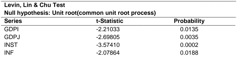
Analysis of Panel Unit Root Test
Licensed under Creative Common Page 186 Chu (LLC) panel unit root test on the variables over 1995-2014.Table 4 below summarizes the results.
Table 4: Panel Unit Root Test Results
Levin, Lin & Chu Test
Null hypothesis: Unit root(common unit root process)
Series t-Statistic Probability
GDPI -2.21033 0.0135
GDPJ -2.69805 0.0035
INST -3.57410 0.0002
INF -2.07864 0.0188
The Levin, Lin & Chu test displayed above seeks to test the following hypothesis: Ho: Panel data
has unit root (non-stationary) against the alternative hypothesis: H1: Panel data has no unit root
(stationary). The results of the panel unit root test gave a probability of less than 5 percent (0.05) which leads us to reject the null hypothesis of panel unit root in all the variables, suggesting the existence of stationarity in all the variables. The t-statistic measures the size of the difference relative to variation in sample data (calculated differences represented in units of standard error). The greater the magnitude of t-values (either positive or negative), the greater the evidence against the null hypothesis that there is no significant difference and the closer t is to 0, the greater the evidence for accepting the null hypothesis. In our case above, the t-statistic for all the variables suggest that the variation in sample data is significant.
The overall conclusion drawn from the panel unit root test results is that the effect of a shock is temporary and our dependent variable will return to its long-run equilibrium. This means that the results obtained using the both random effects model and OLS are consistent and accurate.
Analysis of Normality Test
Normal distribution test using the Jarque-Bera test seeks to test the null hypothesis Ho: Normal
distribution (both skewness and excess kurtosis are equal to zero) against the alternative hypothesis H1: Non-normal distribution (both skewness and excess kurtosis are not equal to
zero).
Licensed under Creative Common Page 187 tend to skew to the left as can be seen in the figures above. Non-normality is not a cause for concern for this study because the statistical tools used do not require normally distributed data (Gujarati, 2004).
Figure 3: Normality Test Results
Normality test obtained under Ordinary Least Squares estimation method:
Normality test obtained under Random Effects estimation method:
0 5 10 15 20 25
-0.6 -0.4 -0.2 -0.0 0.2 0.4
Series: Standardized Residuals Sample 1995 2014
Observations 100
Mean 6.77e-17 Median 0.010639 Maximum 0.434497 Minimum -0.668857 Std. Dev. 0.169700 Skewness -1.332739 Kurtosis 7.574865
Jarque-Bera 116.8090 Probability 0.000000
0 4 8 12 16 20 24
-0.6 -0.4 -0.2 -0.0 0.2 0.4
Series: Standardized Residuals Sample 1995 2014
Observations 100
Mean 9.14e-16 Median 0.006645 Maximum 0.427730 Minimum -0.656101 Std. Dev. 0.166933 Skewness -1.296083 Kurtosis 7.225923
Licensed under Creative Common Page 188 Analysis of Redundant Variables Test
The table below summarizes the results obtained from the redundant variables test.
Table 5: Redundant Variables Test Results
Redundant Variables Test
Null hypothesis: Unit root(common unit root process)
Series t-Statistic Probability
GDPI GDPJ INF 3.071635 F (3,91) 0.3170
GDPI GDPJ INST 2.520161 F (3,91) 0.0629
GDPI GDPJ EAC 2.520161 F (3,91) 0.0636
INF INST EAC 1.075236 F (3,91) 0.3635
The redundant variables test displayed above seeks to test the following hypothesis: Ho: The
additional set of variables is jointly significant against the alternative hypothesis: H1: The
additional set of variables is not jointly significant.
The results of the test for infrastructure, membership to the EAC and institutional quality all gave a probability of more than 5 percent (0.05) which provides no evidence to reject the null hypothesis that the additional set of variables are jointly significant. This gives us confidence that the variables added to the basic gravity model were important in explaining the factors that influence bilateral trade flows in Kenya.
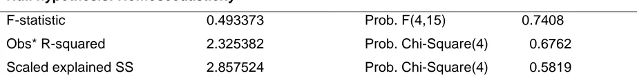
Analysis of Heteroscedasticity Test
The heteroscedasticity test seeks to test the following hypothesis: Ho: Homoscedasticity
(homogeneity of variance) against the alternative hypothesis H1:Heteroscedasticity
(non-(homogeneity of variance)
Table 6: Heteroscedasticity Test Results
Heteroscedasticity Test: Breusch-Pagan-Godfrey
Null hypothesis: Homoscedasticity
F-statistic Obs* R-squared Scaled explained SS
0.493373 2.325382 2.857524
Prob. F(4,15) 0.7408 Prob. Chi-Square(4) 0.6762 Prob. Chi-Square(4) 0.5819
Licensed under Creative Common Page 189 Analysis of Serial Correlation Test
The serial correlation test seeks to test the following hypothesis: Ho: There is no serial
correlation in the residuals against the alternative hypothesis H1: There is serial correlation in
the residuals.
Table 7: Serial Correlation Test Results
Breusch-Godfrey Serial Correlation LM Test
Null hypothesis: No serial correlation in the residuals
F-statistic Obs* R-squared
0.476217 1.365257
Prob. F(2,13) 0.6315 Prob. Chi-Square(2) 0.5053
The results of the test displayed above gave a probability of more than 5 percent (0.05) which provides no evidence to reject the null hypothesis and therefore we can conclude that there is no serial correlation in the residuals.
Analysis of Multicollinearity Test
A large variance inflation factor indicates the presence of multicollinearity while a small factor indicates absence of multicollinearity. The table below summarizes the findings from the multicollinearity test.
Table 8: Multicollinearity Test Results
Variance Inflation Factor
Variable Coefficient VIF
GDPI 0.38816 1.26
GDPJ 0.51020 1.67
DISTIJ -3.44871 1.94
INST 0.36105 1.66
INF 0.10937 1.18
EAC -0.03171 1.16
Licensed under Creative Common Page 190 SUMMARY OF FINDINGS
Summary based on GDP and Distance
The results showed that the gravity model was very successful in explaining the pattern of Kenya‟s bilateral trade flows as coefficients of the standard gravity model variables (domestic and foreign incomes and distance) were found to be robustly consistent with the predictions of the model. Specifically, Kenya‟s total trade flows were found to significantly increase with improvement in domestic and foreign GDPs and diminish significantly with distance.
Summary based on Linder hypothesis vs. Heckcher-Ohlin hypothesis
The pattern of Kenya‟s bilateral trade flows was found to strongly follow the Linder hypothesis, instead of the Heckcher-Ohlin hypothesis. This finding is based on the fact that the coefficient of both domestic and foreign income robustly showed up to be positive and statistically significant in all the models estimated. This suggests that Kenya exports to and trades more intensively with countries with similar per capita income, factor endowments and demand structures. As the theory of overlapping demand predicts, wealthy nations trade with other wealthy nations and poor nations trade with other poor nations.
Summary based on Institutional Quality
The quality of Kenya‟s domestic institutions was found to positively impact the country‟s trade flows. The quality of institutions was proxied by the corruption perception index with Kenya scoring 25 on a scale of zero to one hundred (with zero perceived to be highly corrupt and one hundred very clean). The empirical results are proof that the quality of domestic institutions can create or destroy incentives for individuals to engage in trade and for Kenya‟s case; the better the quality of domestic institutions, the larger the volume of bilateral trade flows.
Summary based on membership to the EAC
The impact of regional integration was found to be positive though statistically insignificant. Membership to the East Africa Community fosters bilateral trade flows. Deductively, this gives an indication that efforts geared towards promoting intra-regional trade in the EAC sub-region have positive effects on trade flows between the member countries.
Summary based on Infrastructure