©EDP Sciences, 2009
DOI: 10.1140/epjconf/e2009-00915-x
T
HE
E
UROPEAN
P
HYSICAL
J
OURNAL
C
ONFERENCESApplications of stable isotope analysis to
atmospheric trace gas budgets
C.A.M. Brenninkmeijer
Max-Planck-Institute for Chemistry, Mainz, Germany
Abstract. Stable isotope analysis has become established as a useful method for tracing the budgets of atmospheric trace gases and even atmospheric oxygen. Several new developments are briefly discussed in a systematic way to give a practical guide to the scope of recent work. Emphasis is on applications and not on instrumental developments. Processes and reactions are less considered than applications to resolve trace gas budgets. Several new developments are promising and applications hitherto not considered to be possible may allow new uses.
1 Introduction
This synopsis presents applications of stable isotope analyses in atmospheric chemistry to supply information for non-isotope-experts to more readily understand scope and potential. It is meant to be a practical guide for elucidating a specialized set of methods as applied to atmospheric chemistry. The importance of the biosphere including soils for atmospheric processes means that the methods also apply to certain biogeochemical issues. The set of isotope methods and applications is rapidly becoming more complex. In many cases the development was driven by isotope experts looking at atmospheric applications. However, stable isotope analyses will most likely grow in the number of applications originating in atmospheric chemistry. Here the judgement about usefulness will be made quickly. In this paper the emphasis is on how trace gas budgets can be resolved. In many papers on this theme, statements like “constraining trace gas budgets” are tabled, but in many cases there is a long way to go. At the best, budget calculations can be constrained. There also is a need for clarity, certainly considering some confusion that existed considering subtle effects that were discovered. Altogether, there are many fascinating new developments.
It is well known that the subtle stable isotope variations in natural systems on Earth pro-vide a wealth of information. In particular in palaeo-climatology one wonders what we would have known about past temperatures not having had stable isotope information. It is like Radiocarbon dating that about 50 years ago started to overthrow some of the often ingenious guesswork of estimating ages of the successive civilizations in the old continent. What were the temperatures 20,000 years ago? The18O/16O ratio of oxygen in water molecules in polar ice or of oxygen in carbonates deposited on the ocean floor that long ago is the source of quantita-tive information. With lower polar temperatures less18O in accumulated ice. When marine life produces shells, small and big alike, remarkably, the carbonate is in a temperature-dependent non-biological isotopic equilibrium with the local ocean water. What about applications in the atmosphere?
Applications in atmospheric chemistry and biogeochemistry are generally of quantitative nature and several fundamental new insights have been obtained. When dealing with atmo-spheric processes, emissions of trace gases, their transport, mixing and in the end their rem-oval, are considered. Not forgotten should be that also aerosol are subjected to isotope analyses. Anyway, considering the sources of trace gases we have the isotopic composition depending on
Article published by EDP Sciences and available at http://www.epj-conferences.org
biological, chemical and physical processes. For instance methane has a range of isotopically distinct sources. Next, methane emitted from these sources is transported and mixed through-out the atmosphere. At the same time, methane is broken down by mainly the hydroxyl radical (OH), and the mixture from the different sources is gradually modified. What is left over gets heavier. Figure 1 shows an example for carbon monoxide, CO. Note that the advantage of isotope studies is that one approaches the cycle of a trace gas at the process level. A totally different approach is based on concentration measurements in particular satellite based obser-vations. Here processes cannot be studied that well. Compared to concentration measurements only, one has a direct coupling to the actual process. These processes, for instance those of the sources processes themselves can be studied further using the isotopic tracers.
Progress in this field has bee enormous. Measurements have become exceedingly precise, down to 0.005‰. Thus for instance variations in the∼1.1% natural abundance of13C as small as 5 ppm are detectable. Measurements are now mostly based on GC techniques, i.e. in a flow of carrier gas (helium), and not on transfer under vacuum in a dual viscous inlet system. This has meant smaller samples and more analyse at the same time. Before systematically visiting the various trace gases from an isotopic point of view we introduce and comment on essential concepts. In this article we must be brief and thus cannot do justice to all isotope work on all gases. Mostly recent work is quoted and analytical info is omitted. Recent reviews are [1–3].
2 Basic concepts
The rare isotopes of the lighter elements (here H,C,N,O,S) are of low abundance. That means that isotopic composition does NOT affect processes. Only for chlorine, where 37Cl happens to be ∼25% with the abundant isotope 35Cl being ∼75%, can changes in isotopic composi-tion really change the bulk behaviour. In all other cases, isotopes are mere tracers. It also means that doubly substituted molecules are very rare. For H2, DD would statistically be only ∼(0.015%)2 abundant. Later we will see that deviations from this statistical distribution may be interesting (clumped isotope analysis).
Isotope effects are small. Only for hydrogen do large effects (say 50%) occur. Here the reason is that the 2 isotopes Deuterium (D) and Protonium (simply H) have large relative mass differences. The isotope ratio is expressed relative to a standard, for instance ocean water for
18O and D present in water samples. The delta notation is used which gives the per mil relative
deviation. Delta values are not additive quantities.
The isotope ratios are on the basis of atomic ratios. This is immediately clear when we look at the example hydrogen. It is easy to see that the ratio HD/H2is twice the D/H ratio. Here we add that measurements are based mostly on stable isotope ratio mass spectrometry which in this case means comparing a beam of HD+ ions (mass 3) with the main beam of H+2 (mass 2) ions. Also laser based methods exist for D,13C and18O. The D/H ratio of atmospheric water vapour can even be measured using remote sensing from outside the atmosphere.
Because stable isotope effects are small, their measurement (necessarily mostly) by stable isotope ratio mass spectrometry has always been tedious and elaborate. A breakthrough has been the development of continuous flow IRMS. Here the gas to be analysed is analysed like a GC effluent, where the isotope ratio mass spectrometer has been “degraded” to a mere detector. Thus the needed high precision and accuracy have been achieved for small amounts of analyte gas carried in a flow of helium. This has revolutionized IRMS applications (compound specific isotope analysis), also in atmospheric applications. Note that nearly always the trace gas is transformed into a gas suitable for isotope analysis. Thus oxidation, reduction, and pyrolysis are used. To give an example, the D/H ratio of CH4 is determined by converting CH4 to H2 by pyrolysis. The high temperatures needed make this rather difficult, but direct measurement of CH4 gives for mass 17 (M/Z) information about 13C and D together. The variations in the rare D isotope cannot be resolved this way readily.
Proper nomenclature is needed. For instance13C is the rare stable isotope of carbon, with
12C being the main, or abundant isotope. Atmospheric methane gas has a 47‰lower13C/12C
depleted in13C. Isotope fractionation in the bacterial processes forming CH4favours formation of12CH4 over13CH4. These molecules are two isotopologues of methane. Isotopomers are like isomers.
Essential are the processes that modify isotope ratios. The main distinction in types of isotope fractionation is that between equilibrium and kinetic isotope effects. Equilibrium isotope effects in chemical reactions are easier to calculate that kinetic effects. Spectroscopic data reveal bond strength parameters and can be used to calculate the partitioning ratios. Physical processes are generally simpler to calculate, for instance the kinetic isotope effects for18O,17O and D in the diffusion of water vapour in air. Chemical reaction, photolysis, diffusion, phase transition, all induce isotope effects.
Nearly all isotope effects are mass dependent. This sounds trivial, then what else would drive different behaviour of stable isotopes but their mass? Electron spin effects underlie certain isotope fractionation processes (e.g. spin forbidden transitions). However, mostly it is merely mass. If an element happens to posses at least 3 stable isotopes, one can verify mass dependence directly because the fractionation for a mass difference of 2 units must be double that for a mass difference of 1 unit. Thus the change in enrichment or depletion for 18O is twice that for17O.
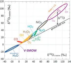
If this rule is broken, and it is severely violated for ozone (O3), one speaks of Mass Inde-pendent Fractionation (MIF). In fact the enrichment in ozone is for 17O almost the same as for18O, which remained a big mystery for years. This one to one relationship was called MIF. But it is not exactly 1.0. Does mass play some role, and is it not totally mass independent? The expression MAF (Mass Anomalous Fractionation) has been coined, with the remark that it perhaps better should not be used. Also MAD (Mass Anomalous Fractionation) has been proposed. Here we advice to use the expression MIF when the fractionation clearly deviates from the expected mass dependence. Ozone is a clear case. Molecules that “inherit” MIF from ozone, for instance NO2because it is formed from O3+ NO, can be said to exhibit MIF.
Some confusion existed at times when this slope of nominally 0.5 for 17O fractionation relative to that for 18O was not well known, or the processes causing fractionation were not well identified. At times one was not always sure whether deviations between measured17O/16O ratios and the ratios expected on the basis of the18O/16O ratio were due to MIF, or just due to different slopes [4]. For small differences one has to be careful to attribute an anomaly to MIF. In other words deviations do not imply that an unusual fractionation process is at work. Since then different slopes have been measured accurately and these agree with the val-ues calculated for mass dependence. The following slopes haven been determined for selected processes with enormous precisions: Waters [5] 0.528, Diffusion of water vapor [6] 0.5184, res-piration [7] 0.518, minerals [8] 0.5247.
Going into more and more detail, one started to consider where in a molecule the isotopic substitution has taken place. The best example is nitrous oxide, N2O. Being structurally NNO, a 15N atom can be in position one or position two [9]. These two isotopomers are these days routinely measured and give valuable additional information for the complex cycle of N2O.
Going even further, recently one has started to seriously address with careful measurements questions like “is the18O content of 13CO2 is the same as that of12CO2?” This is now called “Clumped Isotope Analysis” (CIA [10]). Thereto, in a mass spectrometer, not merely the com-mon masses 44, 45 and 46 are to be measured, but also mass 47. This is only one example. The question is how to use deviations from non-stochastic (statistical) distributions of isotopes.
Not discussed here is the fairly extensive work on D and 18O in H2O. Traditional use was for hydrological applications. Presently, also using measurements by sensors on satellites, work focuses on climate aspects and transport of H2O into the stratosphere. Amazing discoveries and applications have been made by Luz, Barkan and co-workers [11]. A range of subtle mass dependent effects have been studied, giving the traditional MD fractionation effects a new lease on life. The interested reader is referred to their extensive, accurate, often amazing work on processes of diffusion, evaporation and plant physiological processes.
Fig. 1. Schematic to illustrate the use of isotopic information to study the atmospheric cycle and budgets of trace gases, here CO. Fractionation processes “inside” the sources determine the “source signature”. This can be complex reactions, for instance the oxidation processes of isoprene. Not all fractionation processes inside this source of CO are known, but characteristic values are expected, which may depend however on temperature and levels of NOx. Also CO from biomass burning has isotopic compositions depending on a host of processes. As indicated CH4 + Cl produces CO strongly depleted in13C (by about – 80‰). This provides an excellent method to check for the importance of this reaction in the marine boundary layer as it has already been identified in the stratosphere (during ozone hole conditions). The mix of CO from the different sources is modified by the kinetic fractionation in reaction with mainly OH, and to complicate the issue, fresh CO is added continuously from CH4 oxidation and the other sources. Few air masses remain isolated. Here the help of modellers is really needed to figure out the complex interplay. Also source studies are needed for many such applications as illustrated here.
are being done, or will be done in the near future. Some effects are rather complex, yet can be fascinating.
Hydrogen, mass 2, H2, HD
Atmospheric hydrogen has a lifetime of∼1.4 year and a concentration of 0.5 ppmv. It is pro-duced in the atmosphere mainly by the photolysis of formaldehyde (HCHO) which itself is an incompletely oxidized intermediate compound. Hydrogen also is emitted by surface sources, namely fossil fuel combustion, biomass burning, nitrogen fixation and oceans. It is removed by hydrogen atom extraction in OH + H2, but rather slowly. This photochemical sink can be directly calculated because we know OH and the reaction rate constant. However, the removal by soils is complex. Sources are likewise hard to estimate.
An increase in H2, may lead to an increase of this gas in the stratosphere, where it is oxidized to water. Increased water in the stratosphere is undesirable because of cloud formation with various bad consequences (ozone loss on polar stratospheric cloud ice particles). This is of potential concern as H2 has been considered as an energy carrier in the future. The idea that car engines using H2 would mainly emit H2O (not the greenhouse gas CO2) has appealed to politicians (cars “running” on water) and some funding has been made available for research.
Hydrogen does not decrease with altitude crossing from the troposphere into the stratosphere. This strange effect is mainly caused while H2 is still formed from CH4 oxida-tion in the stratosphere, but the effective soil sink is missing here. Thus a weaker source, but concomitantly a much weaker sink. Also strange is the strong D enrichment in the stratosphere which was modelled by Mar et al. [14] after measurements had revealed this effect. The entire process tracing isotopic composition of H2 produced via HCHO starting with CH4 is complex. Rhee et al. [15] used D/H measurements of tropospheric H2collected by aircraft to calculate the overall D enrichment. This enrichment is a linear combination of the small enrichment caused by fractionation in the large soil sink (∼88 Tg/yr), and the large fractionation by the smaller photochemical sink H2+ OH (∼19 Tg/yr). Because the abundance of OH and the large fractionation (0.58) are known, and because the soil fractionation (only 0.943) is known, the soil sink strength can be calculated. This is a clear example of the use of stable isotopes for trace gas budgets.
It is expected that more isotope measurements of atmospheric H2 and sources of H2 will be conducted in the near future for the purpose of better understanding its budget. As Rhee [15] pointed out, global warming increases the soil sink strength, which has to be monitored. Here isotope analyses can truly help to distinguish between changes in sources and sinks.
Methane, mass 16, CH4,13CH4 and CDH3
Methane has a lifetime of∼9 years and a concentration of∼1.75 ppmv. It is emitted by surface sources, namely wetlands, rice paddies, ruminants (all because of anaerobic bacterial processes) and fossil fuel related sources (e.g. coal mining) and combustion and biomass burning. Sources are manifold and difficult to quantify. It is mainly removed by OH + CH4. Cl + CH4is a minor sink, that needs further quantification.
The increase in CH4 harbours 3 concerns. 1) It is a greenhouse gas with an impact com-parable to that of CO2. 2) It acts like a “Troyan Horse” that upon entering the stratosphere delivers, by oxidation, H2O in the stratosphere. More moisture here leads to changes in tem-peratures and ice cloud formation causing ozone losses. 3) It is throughout the atmosphere the main reaction partner of OH (the atmosphere’s natural powerful bleaching agent). It burdens this oxidative capacity. If we can better control the emissions of this gas, humankind would book another tangible progress in abating global change.
Important is the history of CH4 variations in the Earth’s atmosphere in relation to past climate changes. These variations can be measured in air extracted for ice core sections. This information from the past is so valuable that isotopic analysis of CH4 is mandatory. Thus studying the present isotopic composition of all sources implies that we can better unravel the past, including possible changes in climate triggered or driven by methane [16].
researchers have reported that they have seen evidence for the reaction with Cl, which induces a large KIE. However this needs further confirmation. There are too few D measurements for atmospheric CH4 a problem that needs to be addressed. The link with OH is of importance because a change in OH would change13C and D in CH4. Conversely, these may allow conclu-sions about variations in OH. Most applications try to use13C and D to better estimate the many sources of CH4. It is expected that isotope analysis of atmospheric CH4will be continued, although some programs were terminated.
Carbon monoxide, CO, mass 28, 13CO, C17O, C18O, 13C18O
CO has a lifetime of weeks to months depending on latitude and season. Therefore temporal and spatial variations are large being between 35 (Antarctic summer) and 200 ppbv (Arctic winter). The turnover of CO at∼2600 Tg per year is larger than that of CH4.Sources are fossil and biofuel fuel combustion, biomass burning, forest and savanna fires. Large inter-annual variations occur (e.g. during El Ni˜no years with more biomass burning). CO also is produced in the atmosphere in the photochemical oxidation of CH4 and other hydrocarbons. About 5% of CO is removed by soils, with CO + OH being the main sink. This pressure dependent reaction has been extensively studied, but is not yet fully understood.
An increase in CO does burden the OH based oxidative capacity of the atmosphere. However, it seems that the CO increase has been less vigorous in recent years. Fuel efficiency, catalytic converters, increased use of methane play a role here. This is good news because CH4 may be removed faster when CO emission decrease. The diatomic molecule CO itself has no significant greenhouse properties.
The multiple sources, the OH sink, the large turnover, the large variability all render CO isotope analysis useful. If future work shows that CO remains trapped in ice cores without being slowly modified or contaminated, there are exciting possibilities to reconstruct aspects of past atmospheric chemistry. The carbon KIE for CO + OH is small. However δ13C(CO) varies between−31 and−25‰. Low values occur at the end of summer, when CO values are low and the relative fraction of CH4 derived CO peaks. Given that the KIE in CH4 + OH is ∼ −5‰and that δ13C(CH4) = −47‰, CH4 derived CO is with −52‰well below that of organic matter. This explains the large seasonal cycle in13C.
The seasonal cycle for 18O also is large, but here the KIE is the main driving mechanism. Interestingly in CO + OH, C18O reacts almost 10 text per thousand faster. The further away from sources, the more depleted the remaining CO becomes. In autumn δ18O has reached its lowest values. Not known is howeverδ18O of CO from CH4 oxidation. In view of the complex calculations needed, laboratory experiments are advisable [17].
May the inverse isotope effect for C18O be surprising, the behavior of17O in relation to18O is a true mystery. Atmospheric measurements show that C17O behaves more normal in that it has a weak KIE, and not inverse. Laboratory experiments of this reaction have shown that the common mass dependence is violated.
It is expected that isotope analyses of atmospheric CO will continue to be made in greater detail (including∆17O). Clumped isotope analyses of CO have been reported by Eiler’s group. The prospect to apply all these isotope analyses to ice cores and firn air are good, and such would mean doing true palaeo atmospheric chemistry. The history of biomass burning and the oxidative capacity may be reconstructed to some degree. There is no other such information.
Formaldehyde, HCHO, mass 30, HCDO, H13CHO, HCH18O
HCO. In the latter case no H2formation takes place. The other main sink for HCHO is reaction with OH.
Despite its importance, there are comparatively few formaldehyde concentration measure-ments. Moreover, measuring the isotopic composition of atmospheric HCHO is a true analytical challenge [18]. HCHO derived from CH4 oxidation should be strongly depleted in13C and D. This will give a useful source signal. Also the sink reactions give information. Laboratory experiments concerning isotope fractionation caused by photolysis [19, 20], and reaction with OH, Cl, Br, and NO3radicals [21] have been carried out. Normal and inverse isotope effects were observed. This is of interest in the fundamental theoretical work of understanding isotope effects. A practical application is in understanding the isotopic composition of H2 in the troposphere and stratosphere [14].
It is expected that few, if any, larger sets of the isotopic composition of atmospheric HCHO will become available due to the great analytical difficulty. Optical (in situ) measurements would have a better chance.
Ethane, mass 30, C2H6,13CCH6, C2DH5 (and other hydrocarbons)
Hydrocarbons form a family of mostly anthropogenic trace gases having short lifetimes (ethane is comparable to CO) and serving as tracers for chemistry and transport. Their concentrations are below 0.5 ppb, their lifetimes are short to very short (e.g. C5H12), and their impact on chemistry small. Nevertheless their cycles should be understood. As tracers that are continu-ously oxidized at differing rates they allow estimates of the photochemical ages of air masses, and in some cases they give information of whether Cl or Br played a role or not. Isoprene, which is emitted in large quantities by vegetation is of importance to atmospheric chemistry. It reacts with O3 and OH, but only few13C studies are known.
Anticipating their use as tracers, the group of Rudolph [22] has carried out many laboratory studies on the kinetic isotope effects of hydrocarbons. Applications have been made using13C by Yoshida [23] and his group. The budgets of these gases over the ocean have been studied. Reactions with OH and Cl can be studied when one considers an air mass as an isolated unit from which a hydrocarbon disappears.
The inherent useful aspect of stable isotope is that, unlike the traditional use of a set of different hydrocarbons, only one hydrocarbon has to be considered on its own. This means that one has eliminated uncertainties concerning a change in the emission ratios within the set hydrocarbons. The concept “chemical clock” has been introduced. The isotope ratio changes are for a single species. Surprisingly, as Rudolph [24] showed, small fractionation factors are more useful than large fractionation factors. We refer to the original paper for an explanation. This aspect is not intuitive. On the other hand, large isotope effects show clear signals, and it is hoped that there will be more D/H hydrocarbon studies despite their greater analytical difficulty.
Oxygen, O2, mass 32,18OO, 17OO
There is a long standing interest in atmospheric molecular oxygen. Its lifetime is∼103 years, being produced by photosynthetic plants and consumed by respiration, burning and combustion. The18O(O2) enrichment of 23.5‰(V-SMOW) is named the Dole effect. Its cause lies mainly in respiration that discriminates “consumption” of18OO by∼20‰. Understanding the isotopic composition of O2 requires global models incorporation the biosphere [25].
transferred to some degree to CO2. This in turn exchanges O isotopes with H2O (leaf, soil and ocean water mainly), which constitutes a huge reservoir [26, 27]. In effect, an excess of 17O is taken from the large O2reservoir and deposited in the very large H2O reservoir, thus depleting air O2 in 17O. There is a discussion whether this photochemical effect is the only source of the17O depletion and the interested reader must carefully consult the various papers on this complex issue.
Nitrous oxide, N2O, mass 44,15NNO, N15NO, NN17O, NN18O
N2O has a lifetime of roughly 100 years and a concentration of presently∼320 ppbv, tendency rising. Given the long lifetime it has a very weak seasonal cycle, and the same obviously applies to isotopic changes. Sources are oceans and soils and to a lesser degree combustion processes. It sink is in the stratosphere, where is decreases with altitude. It undergoes 2 sink processes here, one is photolysis to NO and O, or N2, and O, the other is reaction with O(1D) to 2 NO molecules. All N2O produced at the surface of the planet must be “digested” through these reaction channels taking place in harsh photochemical environment of the stratosphere.
The concern about the increase in N2O due to land use changes and the use of fertilizers is twofold. It is a long lived greenhouse gas. Second, the production of NO in the stratosphere affects ozone levels there.
There has been enormous progress in stable isotope studies of N2O, covering source process (which are very complex), lab studies, and many atmospheric measurements in the stratosphere and troposphere. As a result, the budget of N2O has indeed become very much better known. Known are today, the 15N isotopic composition for both positions in the molecule (2 iso-topomers), the18O composition, and a small degree of MIF. In the latter case it is difficult to discern the true cause for a small excess in17O. Is it due to unknown sources in the atmosphere involving O3, or due to source processes?
Like mentioned for O2, the proper selection of a reference for 17O deviations (that is the proper δ17O – δ18O relationship for the relevant range of values) is important. The use of a MDF value of 0.528 (waters) will lead to apparently reduced ∆17O values compared to using commercial N2O gases.
Carbon dioxide, CO2, mass 44,13CO2, C17OO, C18OO, 13C18OO
This gas needs little introduction. Its main feature are the huge natural fluxes on which the unabated man made flux is superimposed. Isotope measurements have been carried out for over 5 decades, and have helped to better understand its budget. The enrichment in18O and MIF that take place in the stratosphere are well understood, although fundamental work on the exchange processes involving the short lived CO3 complex continue [28].18O in tropospheric CO2 is an extremely useful indicator reflecting the exchange with water in plants, soils and oceans. Changes in temperature (via the fractionation constant), in relative humidity (via the kinetic isotope effect in evaporation) and in the hydrological cycle affect18O in a complex but distinct manner. 13C is nearly always well correlated wit the inverse concentration, reflecting photosynthesis, respiration and fossil fuel related emissions. Large data sets for CO2 concen-tration and13C and18O as being established by NOAA-ESRL will indeed help to “constrain” the CO2 budget and to follow effects of man’s impact on nature.
New possibilities are based on the “clumped isotope analysis” mentioned before. Affek et al. [29] have analysed mass 47 abundances in CO2extracted from urban air, car exhaust, and human breath. At high temperatures, thermodynamic equilibrium exists, other process show deviations that although being small (sub per mil), may be useful.
Nitrogen oxides (NO), (NO2), nitrate
capacity of the atmosphere. When NO increases the chemistry speeds up. Given the presence of reduced gases (CO, hydrocarbons) it leads to the formation of photo chemical smog, and atmospheric chemists seem to divide the atmosphere in two regimes of low NOx (ozone loss) and high NOx (ozone producing).
Clearly, isotope studies of NO would be valuable to understand its complex chemistry. This is however, at the time being, not possible. NO concentrations are very low, and the gas reacts immediately with O3. Only sunlight forms back NO. Both NO and NO2 measurements are difficult, not to mention isotope analyses. The interesting aspect is the reaction with O3, which transfers the MIF signal from O3 to NO2 and NO [30].
However, there is great progress in analysing nitrates, the end product of the oxidation processes. Nitrates can be collected as aerosol material on filters and are successfully subjected to17O,18O and15N analyses. Insofar nitrates do not exchange O atoms with water the signal is retained. This implies the interesting possibility to study the NO-nitrate cycle in the polar regions in the past using ice core analyses.
Ozone, O3, mass 48,17OO2,18OO2, O18OO, and many more
Ozone needs little introduction as its roles as a shield against UV radiation, as a greenhouse gas, as a precursor of OH, and as pollutant (photochemical smog) are widely documented. It is the most monitored and thoroughly studied atmospheric trace gas next to CO2. Ozone is formed by the Chapman cycle in the stratosphere and everywhere continuously photolysed at a high rate and formed back by O reacting with O2. This process causes a large enrichment in18O and the surprisingly almost equal enrichment in 17O (MIF). This anomaly propagates through many reactions, as outlined in Figure 2. Tropospheric O3 arises from import from the stratosphere while the photolysis of NO2 to NO and O is the solein situ source. Temperature and pressure differences are the causes for differences in isotopic composition between tropospheric and stratospheric O3.
Isotope measurements of tropospheric O3are hauntingly difficult, because it is so difficult to separate it from air quantitatively. Only 2 experiments are known. Two main aspects about O3 isotope research are to be mentioned. One is that Mauersberger and his group [31] have carried out the most extensive and precise measurements of ozone formation reactions using all sorts of isotope mixtures. Enormous differences in reaction rate constants have been documented. The other is progress in theoretical studies by Markus and co-workers [32] on explaining the enigmatic enrichment of O3. The enrichment of the terminal positions is higher than the overall enrichment. This is of relevance for the transfer of MIF to molecules reacting with O3.
Methyl chloride, CH3Cl, mass 50, 13CH3Cl, CDH2Cl, CH337Cl and many more
The lifetime of methylchloride is ∼1 year. This number is almost as well known as that of methane. The reason is that they share their main sink, namely OH. Methylchloride has a concentration of about 550 pptv. It is emitted by mainly plants, biomass burning, oceans, fungi, salt marshes, coal combustion, wetlands and lesser sources. Special about methylchloride is that it is chiefly produced and consumed in the tropics. This means that it there has a high turnover, and large variability (shorter local lifetime). Tropical values tend to be higher than those at mid and higher latitudes, indicating an excess production there.
Fig. 2.This nice diagram (sometimes called a 3 isotope plot for oxygen) showsδ17O relative toδ18O in a simplified form. The proper parameters to be plotted are ln(1 +δ) values. Values indicated are based on atmospheric measurements, and on model results by Sergey Gromov. In the past it has been difficult at times to use isotopic information. Presently however, modelling studies help quantitative applications enormously. The results even show the oxygen isotopic composition of OH, the very short lived natural bleaching agent of the Earth’s atmosphere. OH measurements belong to the most difficult measurements, yet, models enable a detailed understanding of the chains of isotopic processes in the atmosphere. Apart from H2O (physics only), all effects are traceable to mainly chemical effects. The general Mass Dependent Fractionation line has nominal slope 0.5, but for different processes, the actual values have been calculated and measured, often with surprisingly great precision. This has allowed new applications of mass dependent fractionation. Today we much better know the mass dependence than before. If there are deviations, we have – as Weston points out – to see if it due to different mass dependent processes, or to true deviation. For instance the strange behaviour of CO is due to the MIF in the removal reaction CO + OH. Laboratory measurements of this reaction and atmospheric observations leave no doubt about the role of OH. Work is in progress right now by Markus and co-workers to find the theoretical description of the isotope effects in CO + OH. Also Weston works on this tantalizing problem. All other effects shown here may well be due to MIF originating in ozone propagating through the complex reaction schemes. This picture shows that there are many aspects of the oxygen cycle in atmospheric trace gas budgets to be studied.
It is desirable that considerably more isotope studies are devoted to CH3Cl. For CH3Br, a close relative of this molecule, several isotope studies have been published. For13C studies the gases are combusted to CO2. For D one expects a priori very large effects because only 3 H atoms are present. For D studies, pyrolysis to H2 is needed. Cl isotopes can be studied by using this gas directly with a suitable configuration of ion collectors in the mass spectrometer. In fact, Cl isotopes in minerals and groundwater have been studied by converting Cl to CH3Cl for mass spectrometry.
Carbonyl sulfide, COS, mass 60, 13COS, C17OS, CO36S and many more
by oxidation of oceanic CS2 and DMS, and other sulphurous compounds natural and anthro-pogenic. Direct emissions from biomass burning also are relevant. COS is removed by plants, through oxidation by OH and by soils. Like CO2 it enters stomata upon which a lare fraction is irreversibly lost by hydrolysis accelerated by enzymes. The remaining smaller sink is destruc-tion in the stratosphere through its photolysis. This in turn is a major source of ultimately sulphate, which forms a layer of aersosol known as the Junge layer. In the absence of strong volcanic eruptions (like Mt. Pinatubo in 1991) COS and SO2entering the stratosphere maintain the Junge layer. The COS budget calculations, which differ strongly between the southern and northern hemisphere, have uncertainties and could benefit from isotope studies.
It is desirable that isotope studies are devoted to COS. Its sink reaction in plant leaves render information about COS particularly useful with regard to CO2 fluxes. Analytically the main challenge is its separation from CO2 prior to isotope analysis. COS can be combusted to CO2 and SO2 for isotope analyses on the basis of these gases. Direct analysis of COS (mass 60) may be more rewarding, giving information on13C,17O and 33S (mass 61),18O,34S and
33S +17O (mass 62). We leave it to the reader to combine all masses (2 for C, 3 for O and 4
for S) to find its isotopologues, and to see if the system is determined. If ion collectors for 60, 61, 63 and 63 etc. are not sufficient, fragment ion analysis may help to clarify things like was done for N2O [9].
3 Conclusions
This brief overview explaining the role of trace gases and the scope of isotope analyses should be a compact guide to assess and identify applications. Some promising isotope applications are signalled, which are very much worthwhile to pursue, not only for “constraining” trace gas budgets, but for understanding sink and source processes and may be discovering new effects. Not all gases are mentioned, for instance H2O2. It is noted that sophisticated modelling of isotope parameters in 3D chemistry-transport models of the atmosphere is increasingly becom-ing available. This allows quantitative applications, and shows how isotope applications have reached their “adult state”. Finally it is concluded that in particular the important reconstruc-tion of the Earth’s atmosphere past composireconstruc-tion, particularly concerning its oxidative state and trace gas levels using the extremely valuable ice core material, warrants detailed studies using isotopic information for the present atmosphere.
Sergey Assonov is acknowledged for useful discussions and Sergey Gromov for the complex model calculations on isotopic composition of trace gases and for supplying figure 2, which is an update of similar diagrams from various colleagues in isotope research.
References
1. C.A.M. Brenninkmeijer, C. Janssen, J. Kaiser, T. Rockmann, T.S. Rhee, S.S. Assonov, Chem. Rev. 103, 5125 (2003)
2. M.S. Johnson, K.L. Feilberg, P. von Hessberg, O.J. Nielsen, Chem. Soc. Rev.31, 313 (2002) 3. M.H. Thiemens, Ann. Rev. Earth Planet. Sci.34, 217 (2006)
4. R.E. Weston, J. Nucl. Sci. Technol.43, 295 (2006)
5. H.A.J. Meijer, W.J. Li, Isotopes Environ. Health Studies34, 349 (1998) 6. E. Barkan, B. Luz, Rapid Comm. Mass Spectrom.21, 2999 (2007) 7. B. Luz, E. Barkan, Geochim. Cosmoch. Acta69, 1099 (2005)
8. M.F. Miller, I.A. Franchi, M.H. Thiemens, T.L. Jackson, A. Brack, G. Kurat, C.T. Pillinger, Proc. Nation. Acad. Sci. USA99, 10988 (2002)
9. C.A.M. Brenninkmeijer, T. Rockmann T., Rapid Comm. Mass Spectrom.13, 2028 (1999) 10. J.M. Eiler, Earth Planet. Sci. Lett.262, 309 (2007)
11. A. Landais, E. Barkan, B. Luz, Geophys. Res. Lett.35(2008)
14. K.A. Mar, M.C. McCarthy, P. Connell, K.A. Boering, J. Geophys. Res. Atmos. 112 (2007) doi:10.1029/2006JD007403
15. T.S. Rhee, C.A.M. Brenninkmeijer, T. Rockmann, Atmos. Chem. Phys.6, 1611 (2006)
16. K.R. Lassey, D.M. Etheridge, D.C. Lowe, A.M. Smith, D.F. Ferretti, Atmos. Chem. Phys.7, 2119 (2007)
17. R.E. Weston, J. Phys. Chem. A105, 1656 (2001) 18. A.L. Rice, P.D. Quay, Anal. Chem.78, 6320 (2006)
19. T.S. Rhee, C.A.M. Brenninkmeijer, T. Rockmann, Atmos. Chem. Phys.8, 1353 (2008)
20. K.L. Feilberg, M.S. Johnson, A. Bacak, T. Rockmann, C.J. Nielsen, J. Phys. Chem. A111, 9034 (2007)
21. K.L. Feilberg, M.S. Johnson, C.J. Nielsen, J. Phys. Chem. A108, 7393 (2004) 22. R. Iannone, R. Koppmann, J. Rudolph, J. Atmos. Chem.58, 181 (2007) 23. H. Nara, S. Toyoda, N. Yoshida, J. Atmos. Chem.56, 293 (2007) 24. J. Rudolph, E. Czuba, Geophys. Res. Lett.27, 3865 (2000)
25. G. Hoffmann, M. Cuntz, C. Weber, P. Ciais, P. Friedlingstein, M. Heimann, J. Jouzel, J. Kaduk, E. Maier-Reimer, U. Seibt, K. Six, Global Biogeochem. Cycles18(2004)
doi:10.1029/2003GB002059
26. B. Luz, E. Barkan, M.L. Bender, M.H. Thiemens, K.A. Boering, Nature400, 547 (1999) 27. J.R. Lyons, Geophys. Res. Lett.28, 3231 (2001)
28. K.A. Boering, Geochim. Cosmochim. Acta69, A444 (2005)
29. H.P. Affek, X.M. Xu, J.M. Eiler, Geochim. Cosmochim. Acta71, 5033 (2007)
30. J. Savarino, S.K. Bhattacharya, S. Morin, M. Baroni, J.F. Doussin, J. Chem. Phys. 128(2008) doi:10.1063/1.2917581
31. C. Janssen, J. Geophys. Res. Atmos.111(2006)doi:10.1029/2006JD007768
32. R.A. Marcus, Mass-independent oxygen isotope fractionation in selected systems. Mechanistic considerations in Advances in Quantum Chemistry: Applications of Theoretical Methods to
Atmospheric Science (2008), pp. 5–19