Design Of A Low Cost System For PID Control For Temperature Control

(1)

2058

Design Of A Low Cost System For PID Control

For Temperature Control

Wilver Auccahuasi, Juan Grados, Nicanor Benites, Santiago Rubiños, Celso Pascual, Miltón Martinez

Abstract: The present research work is carried out to design a system which allows to gather information and control the necessary temperature in a poultry incubator through the type K Thermocouple sensor. In this degree project, the world of artificial chicken incubation is explored, starting from the natural process, establishing the variables, conditions and critical aspects of the process, in order to develop a small-scale artificial incubation system, which different from the processes used in it, guarantee a representative increase in its efficiency, that is, in the number of live chicks obtained

Index Terms: Control, PID, temperature, poultry, system.

——————————  ——————————

1 INTRODUCTION

ince ancient times, the desire to control the environment has been a basic, inherent and innate characteristic of the human being. Man has tried to control natural phenomena, his peers, other living beings, etc. On many occasions presenting negative results for humanity. In parallel, since times as remote as civilization itself, man has always sought to have more objects, goods and acquisitions. As Karl Marx mentions in his work, capital, it is sought that a smaller amount of work acquires the ability to produce a greater amount of use value [1]. This is why diverse technology has been developed throughout history, in order to evolve production systems and discover new ways by which merchandise can be produced with fewer people or in less time than before [2]. The first significant work in automatic control was the James Watt centrifugal speed regulator for the control of the speed of a steam engine, in the eighteenth century. [3] In 1922, Minorsky worked on automatic controllers for boat guidance, and showed that stability can be determined from the differential equations described by the system. [3]

2 METHODS

Y

MATERIALS

The problem is basically to characterize well the variable to be measured, in this case the considerations would be the temperature at which the eggs will be, their ventilation, humidity, etc. Once this is done, you must define the cabin for the same (incubator) and the external conditions to which you are exposed, the thermal system that will be used to condition the interior temperature of the same, among others, and as a consequence choose the suitable sensor for the variable to measure.

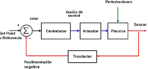
Once all this is done, the first step is resolved. In the next step it will be due to design the power system that will handle the cabin heater and then control system of such power system, which is the PID itself, this is clear using the results of the first item.Once this point is reached, it only remains to calibrate and make adjustments to it.Control system is a set of components that act together to achieve an objective, where the values of one or more variables to be controlled are measured and one or more control variables are applied to correct or limit a deviation from the measured value from a desired value [5]. There are two configurations of control systems: open loop systems, without feedback on the system output, or closed loop, which have feedback and are of interest to the project.A closed loop system is a feedback control system. This configuration "compensates for disturbances by measuring the output response, feeding that measurement to a feedback path and comparing that response with the input" [6]. Similarly, they are more precise and allow greater control of the transient response and error in a permanent state than an open loop system.

Figure 1. Block diagram of a closed loop control system.

The PID control is a unit to create a stable control loop and achieve the desired performance through three types of basic error correction actions: proportional, integral and derivative [7]. PID control in the industry is highly used, because current programming software generally includes libraries or PID control functions.

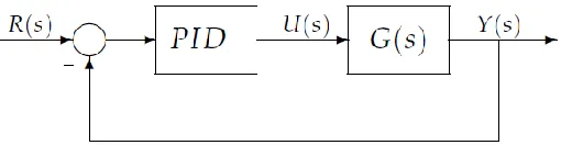
Structure of a PID control. Consider a control loop of an entrance and an exit (SISO) of a degree of freedom: S

_______________________________________

• Wilver Auccahuasi, Centro de investigación en Automatizacion para el Desarrollo, Universidad Nacional del Callao, Perú

• Juan Grados, Centro de investigación en Automatizacion para el Desarrollo, Universidad Nacional del Callao, Perú

• Nicanor Benites, Centro de investigación en Automatizacion para el Desarrollo, Universidad Nacional del Callao, Perú

• Santiago Rubiños, Centro de investigación en Automatizacion para el Desarrollo, Universidad Nacional del Callao, Perú

• Celso Pascual, Centro de investigación en Automatizacion para el Desarrollo, Universidad Nacional del Callao, Perú

(2)

Figure 2. Block Diagram

The members of the PID controller family include three actions: proportional (P), integral (I) and derivative (D). These controllers are called P, I, PI, PD and PID. Proportional Control Action (P): It gives an output of the controller that is proportional to the error, that is, which is described from its transfer function:

( )

p p

C s



K

Equation (1)

Where

K

p, it is an adjustable proportional gain.

A proportional controller can control any stable plant, but it has limited performance and error in permanent regime (off-set). Integral Control Action (I): It gives an output of the controller that is proportional to the accumulated error, which implies that it is a way to control slowly.

0

( )

_i t

( )

u t



K



e

 

d

Equation (2)

( )

i

K

C s

s



Equation (3)

The control signal

u t

( )

has a nonzero value when the error

signal is zero

e t

( )

Therefore, it is concluded that, given a constant reference, or disturbances, the permanent error is zero.

Proportional Control Action - Integral (PI):

It is defined by the equation:

0

( )

_p

( )

p t

( )

i

K

u t

K e t

e

d

T

 





_

Equation (4)

Where

T

i_{, It is called integral time and is the one who adjusts}

the integral action. The transfer function results:

1 ( )

(1

)

PI p

i

C

s

K

T s





Equation (5)

With proportional control, it is necessary that there is an error to have a non-zero control action. With integral action, a small positive error will always give us an increasing control action,

and if it is negative the control signal will be decreasing. This simple reasoning shows us that the permanent error will always be zero. Many industrial controllers have only PI action. It can be shown that a PI control is suitable for all processes where the dynamics are essentially first order. What can be demonstrated in a simple way, for example, by a step test.

Proportional-derivative control (PD) action:

It is defined by the equation:

( )

_p

( )

_{p d}

de t

u t

K e t

K T

dt





Equation (6)

Where

T

d_{It is a constant called derivative time. This action}

has a foresight character, which makes the control action faster, although it has the important disadvantage that amplifies the noise signals and can cause saturation in the actuator. The derivative control action is never used on its own, because it is only effective during transient periods. The transfer function of a PD controller results:

( )

PD p p d

C

s



K



sK T

Equation (7)

When a derivative control action is added to a proportional controller, it allows a high sensitivity controller to be obtained, that is, it responds to the speed of the error change and produces a significant correction before the magnitude of the error becomes too large. Although the derivative control does not directly affect the steady state error, it adds damping to the system and, therefore, allows a larger value than the K gain, which results in an improvement in the steady state accuracy.

Proportional-integral-derivative control (PID) action: this combined action brings together the advantages of each of the three individual control actions. The equation of a controller with this combined action is obtained by:

0

( ) ( ) p ( ) p t ( ) p d

i

K de t

u t K e t e d K T

T

 

dt

 





Equation (8)

And its transfer function results:

1 ( )

(1

)

PD p d

i

C

s

K

sT

T s





Equation (9)

2.1 solution Desing

(3)

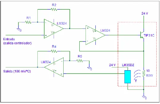
2060 amplifier with a gain of 10 at its output. Since the temperature

range to be controlled is between 35ºC and 45ºC, the output voltage of the conditioner will be between 3.5V and 4.5 V, entering the input range of the acquisition card. The first process, is to perform is to look for the image indicating the area affected by the emergency, the search can be carried out on the portal of the SENTINEL satellite mission. Figure 3. Search of the affected area in the geoeportal of the SENTINEL satellite mission. In figure 3. The process of search of the area of interest is described, this process is important, because by locating the area of interest we can obtain the images of the affected area with different acquisition dates, in image 4 it is presented an acquisition made on October 27, 2015, this image is used as a reference in order to analyze it later.

Figure 3. Electrical diagram of the power amplifier and conditioning circuit.

Once the power and conditioning circuit stages have been designed, the student must go through different stages to reach a valid controller. Next, the plant is identified. Because a thermal system has an increasing monotonic response similar to a first-order system, it is sufficient to introduce a step to the plant and observe the response, from which the necessary parameters for tuning the controller will be deduced. Once a mathematical model of the plant is obtained, a standard controller (P, PD, PI or PID) will be designed based on the characteristics that the controlled system must satisfy.

2.2 Plan identification

An important phase in the design is the identification [3] that aims to obtain a mathematical model that reproduces with sufficient accuracy the behavior of the process. The good behavior of the designed controller will depend on the accuracy of the model obtained. There are two basic methods of identification: analytical identification (modeling) and experimental identification (classical identification). For the modeling, a very specialized knowledge about the technology of the process is required, while for the classic identification (which is the most direct method) it is necessary to apply to the process special signals such as steps, ramps, impulses, sinusoids or pseudo-random signals.

In Eq. 10, K is the gain of the process, td the delay time and τ

the time record. These parameters are obtained from the

response obtained in the identification process before entering the step. For example, a plant described by K = 3, td = 2 sec and τ = 4 sec, before a step input of amplitude 5, will present the answer shown in Fig 4. As you can see the final value is 15, being K = 15/5 = 3, the delay time is clearly seen to be 2 sec and the time constant would be calculated at 63.2% of the final value, that is, at 9.48 corresponding to a τ of 4 sec.

Figure 4. This one that presents a first order plant with delay

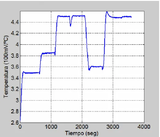
Figure 5. Response offered by the plant for a step of amplitude 0.7

In the same way experiments are done for amplitudes of 0.5, 0.6 and 0.8 (Fig. 5).

From the results obtained, it is observed that the plant is not linear in the operating range, so that a medium transfer

function can be obtained (Ec.10):

3 RESULTS

Once the plant identification is done, some technique will be chosen for the controller design. First you start by applying some empirical technique of tuning the parameters of the controller, such as the Ziegler-Nichols rules or the Cohen-Coon method and then fine tuning is performed to improve your performance. Once the above is done, some classical method is applied to the controller design, in this case the root

location method has been chosen

(4)

Figura 6. Values of controller parameters according to Ziegler-Nichols

The resulting PI or PID controller has the following expression (Ec.3):

By the Cohen-Coon tuning formulas (Fig. 10):

Figure 7. Values of controller parameters according to Cohen-Coon

The resulting PI or PID controller has the following expression (Ec.4):

Looking at Ec.3 and Ec.4, it is seen that there is only a slight difference between the PI of Ziegler-Nichols and that of Cohen-Coon. As for the PID the biggest difference is in the derivative part, which in principle will make the Cohen-Coon PID more cushioned, but slower.

Figure 8. Root geometric place with proportional controller

In Fig. 8 it is observed that the pole that appears in open loop near the origin is in the position s = -1 / 861. If we use the pole cancellation technique, we could eliminate this pole with a zero from the controller and place another pole in open loop at s = 0 (to make the type one system). With this we would obtain as a controller a PI of the form (Ec.5):

The geometric place of the roots (Fig. 9) is now obtained with the code in MATLAB:

Figure 9. Root geometric place with PI controller

It remains to determine the gain KC. To do this, the poles can be placed in a closed loop at the point of separation from the root site using the MATLAB rlocfind command:

MATLAB gives us a value of KC = 0.01. Therefore, the controller will have the expression (Ec.6):

(5)

2062 Undoubtedly, we must not lose sight of the fact that several

approaches have been made (plant transfer function and Pade approximation), so that in practice a fine tuning of the controller must be performed.

Figure 11. Sequence is tested

Figure 10. Root geometric place with PI controller

The project developed is compatible and integrable through the RS232 serial port, which makes it very versatile for programming or viewing from a portable PC. Experimental results show that the diffuse controller is robust in the operating ranges. The temperature has a good response is the transient and stationary state. The controller also worked well despite the presence of disturbances and download changes. Its development cost is cheap which makes it possible to adapt it to control poultry incubators for the purpose of saving electricity.

4 CONCLUSIONS

The process to be followed has been shown for the student to prove in practice the theoretical knowledge about control theory. One of the aspects to highlight is the interest shown by the students and the satisfaction they show when verifying the

proper functioning of the design carried out. Performing a team work, results are compared and the causes that lead to a certain system behavior are searched. Regarding the results obtained, 90% of the students have passed the practice with good results. This is a practice in which many concepts are included, representing for the student a difficulty since it has to see in principle the problem in a global way and then go on reeling and solving the different points to solve that arise. It is a good practice to have the student apply the theory of control to a specific problem and not stay there, in simple control theory, abstract and without practicality. Another point to highlight would be that, given the economic nature of the plant, each student can have one and do the practice without material restrictions.

5 REFERENCES

[1]. K. Marx, El Capital, Tomo 1, Volumen 2, p. 386, México: Grupo editorial siglo veintiuno, 2013. [2]. F. Galiani, Della moneta, pp. 158, 159, 1750.

[3]. K. Ogata, Ingeniería de control moderna, pp. 1, 2, 3, España: Pearson Educacion S.A, 2010.

[4]. Merriam-Webster’s Collegiate Dictionary, 11th ed. 2012.

[5]. K. Ogata, Ingeniería de control moderna, pp. 4, 5, México: Prentice Hall, 1998.

[6]. N. S. Nise, Sistemas de control para ingeniería, pp. 12, 13, México: Compañía editorial continental, 2006.

[7]. J. Manrique de la Cruz, Desarrollo de un control PID wavenet, Tesis de Licenciatura, Universidad Nacional Autónoma de México, 2010.