An Analysis Of The Temporal Evolution
Of Agrarian Prices
María-Encarnación Andrés-Martínez, University of Castilla-La Mancha, Spain José-Luis Alfaro-Navarro, University of Castilla-La Mancha, Spain
Víctor-Raúl López-Ruiz, University of Castilla-La Mancha, Spain
ABSTRACT
At the end of 2007 and principles of 2008 took place the greater nourishing crisis of the last decades. This crisis was caused by a spectacular increase in the prices of some agricultural raw materials and in the costs of the agrarian production. Since the end of 2008 the prices of the agricultural raw materials have decreased with similar intensity as when they raised. In the upward period, the increases of prices quickly were moved to the final consumer prices without great impact in the farmer’s income but when the prices decreased they do not allow seeing so fast in the final consumers prices. In this paper, we analyse the evolution of the agricultural activity results over the last years. In order to do so, we consider the prices of agricultural raw materials and products made with these, without forgetting the production costs. This study analyses the evolution of: the differential between the producer (farmer and stockman) prices and the prices charged for agrarian products to the final consumers and the differential between the producer price and the production cost.
Keywords: agrarian prices, production cost, agrarian income.
1. INTRODUCCIÓN
he trend in food prices sparked a reaction from the public administration to try to control the upturn in the prices of these products. Thus, the Plan of Action in Domestic Trade 2004-2008 established the necessity to increase the transparency of; price formation processes and the information provided to the consumers about these processes.
In this sense, it is striking to observe how low prices paid to farmers coexist with high prices paid by consumers at destination and also how increases in production costs do not result in increases in producer prices. This situation is far too frequent in the Spanish economy. As a result, criticism on behalf of farmers for the low price of their products coexists with prices paid by consumers that are not in keeping with the prices paid to farmers and cattle breeders. (Paz, 2005; and Del Campo, 2006).
The empirical studies about the relationship between agrarian prices at origin and destination can be divided into two large groups: on the one hand, those that are based on the analysis of the evolution of commercial margins (Rebollo, et al., 2006a and 2006b; Cruz, 2008 and Alfaro, et al., 2009); and, on the other hand, the studies that are based on the analysis of temporal series (Peña and Sumpsi, 1980; Cancelo, 1989; Gil and Albisu, 1993; Judez, et al., 1993; Arias, 1999; Kaabia and Gil, 2008). Although, these last ones are trims in the analysis of the one product evolution.
In this paper, using the information on the price of fresh products published by the Spanish Ministry of Industry, Tourism and Commerce (2010) and the information on producer prices and those paid by the farmer and stockman published by the Ministry of Environment and Rural and Marine Affairs (2010), we analyse the temporal evolution of these prices. More specifically, we analyze the evolution of the ratio between the origin and destination prices of fresh products and the ratio between producer prices and those paid by farmer and stockman. In this sense, we consider the viewpoint of the consumer and producer when considering the evolution of the prices that
consumers pay and the evolution of producer prices and those paid to elaborate agrarian products.
2. AGRARIAN PRICES
Mercasa, along with the Ministries of Industry, Tourism and Commerce and Environment and Rural and Marine Affairs, participate in the elaboration of a set of economic indicators that provide precise information about the evolution of prices and commercial margins. The first publishes information related to the weekly prices of 35 nourishing products considered for the period between 2004 and the first weeks of 2010. These prices include: origin prices provided by the Ministry of Environment and Rural and Marine Affairs; wholesaler prices published by MERCASA; and destination prices provided by the State Secretariat of Tourism and Commerce. With these prices, we construct a ratio that makes it possible to compare destination and origin prices.
The prices at origin (PO) are average national prices weighted in the origin market. The weightings are obtained considering the amounts sold monthly in representative markets of different Autonomous Regions. Destination or consumer selling prices (PVP), however, are the weighted national average prices of sale to the public in €/kg, €/dozen or €/unit (Ministry of Industry, Tourism and Commerce, 2010). By means of the quotient between these prices we can obtain a ratio to analyze the evolution of the differential of prices repelled to the consumer with respect to the price paid to the producer at origin. This ratio is calculated as the quotient between destination prices or sale prices to the public (PVP) and prices at origin (PO).
PO
PVP
origin
n
destinatio
Ratio
/
On the other hand, the Ministry of Environment and Rural and Marine Affairs (2010) with the collaboration of the Autonomous Regions elaborate the survey of farmer and stockman (producer) prices. This includes calculating the indices of producer prices and those paid by the farmer and stockman. Thus, the index of producer prices, with base in 2005, is published monthly for different products, the main groupings being as follows:
Vegetable products, including agricultural and forest products. Group A (Agricultural) includes cereals, legumes, potatoes, industrial and fodder crops, citrus potatoes, non citrus fruits (fresh and dry fruits), vegetables, wine and unfermented grape juice, oil, seeds, flowers and ornamental plants.
Animal products, including the groups of cattle for supply (bovine, ovine, goat, pig, birds and rabbits), cattle products (milk, eggs and wool).
The integration of these two great groups (vegetable and animal) gives rise to the general index of farmer and stockman prices.
In addition, the Ministry of Environment and Rural and Marine Affairs publishes a monthly index of prices paid for the different goods and services from current use, including: seeds and shoots, fertilizers, foods of cattle, plant health protection, animal health treatments, conservation and repair of machinery and buildings, energy and lubricants, material and small tools and general expenses. By joining these groups together, we obtain the general index of goods and services of current use (INPUT I). Furthermore, indices take shelter from capital assets: machinery and other equipment and investment. The combination of these two indices gives rise to the general index of capital assets (INPUT II). And, the integration of groups INPUT I and II gives rise to the general index of paid prices by the farmer and stockman.
Through the quotient between the indices of producer prices and those paid by the farmer and stockman we can obtain a ratio to analyze the evolution of the existing margin in the development of the agrarian and cattle activity.
index
price
Paid
index
price
oducer
pricepaid
ice
producerpr
3. DATABASE
For the empirical analysis performed in this paper we have used the weekly prices of 35 nourishing products considered for the period between 2004 and first weeks of 2010. Although, once the data was filtered by excluding some products due to a lack of information, we obtained the weekly prices of a total of 28 products for the period between 2005 and the first 17 weeks of 2010. We also obtained monthly producer price indices and the indices for the prices paid by the farmer and stockman from January 2000 to December 2009.
In relation to the weekly prices at origin and destination for the 28 products, we have calculated the ratio defined previously to analyze their evolution over time. In order to do so, the products considered have been grouped into three categories, which are:
• Meat: calf, lamb, pig, chicken and rabbit.
• Fish: hake, whiting, sardines, anchovies, roosters, horse mackerel, cod, trout, mackerel, salmon, chir and mussel.
• Fruits and vegetables: potato, beet, marrow, onion, bean, lettuce, pepper, tomato, carrot, lemon and banana.
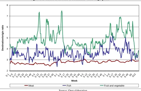
Using the information for each product in each category, we have calculated a ratio by category using an unweighted average. The evolution of these for the three product categories is shown in figure 1.
Figure 1. Evolution of the ratio of destination versus origin prices
2 3 4 5 6 7 8
S 1 S 9S 17S 25S 33S 41S 49 S 5S 13S 21S 29S 37S 45 S 1S 9S 17S 25S 33S 41S 49 S 5S 13S 21S 29S 37S 45 S 1 S 9S 17S 25S 33S 41S 49 S5 S13
Week
Des
tin
a
tio
n
/o
rig
in
r
a
tio
Meat Fish Fruit and vegetable
Source: Own elaboration.
of 0.82, compared to 0.48 for fish and 0.13 for meat. Perhaps, the justification could be that this type of product undergoes more intermediate manipulation between the producer and the final consumer and, therefore, is exposed to a greater presence of abusive commercial margins.
Figure 2 shows the monthly evolution of producer prices and those paid by farmers and stockmen from January 2000 to December 2009. If we analyze figure 2, we can see paid prices are more disperse than producer prices. Thus, the standard deviation of the series of paid prices is 12.13, whereas in the case of producer prices, it is 8.8. In addition, the average value of the index of paid prices in the sample period is more than seven points higher than that of producer prices (100.6 compared to 93.2). Undoubtedly two aspects stemming from the comparison of the series are worth emphasizing; on the one hand, the two series record different trends are observed at the end of the period. While the series of producer prices tends to increase, paid prices tend to fall. This might be good news for farmers if the two series are at least able to balance throughout 2010. On the other hand, since the beginning of 2008 paid prices have been quite distant with respect to producer prices. This situation peaked in August 2008, when the distance between the index of paid and producer prices rose to 36.3 percentage points (135.1 compared to 98.8). While our first appreciation may be positive, if the situation consolidates over the next few months, our second affirmation must be taken with caution because of the increase in costs observed without being offset by an increase in producer prices has reduced the competitiveness of the Spanish farming industry. This situation has led us to define a ratio that compares producer prices to the prices paid by farmers and stockmen paid.
Figure 2. Indices of Producer Prices and Prices Paid
70 80 90 100 110 120 130 140 150
2000
M01
2000
M08
2001
M03
2001
M10
2002
M05
2002
M12
2003
M07
2004
M02
2004
M09
2005
M04
2005
M11
2006
M06
2007
M01
2007
M08
2008
M03
2008
M10
2009
M05
2009
M12
Month
In
d
e
x
Producer prices Paid prices
Source: Own elaboration.
If we consider the tendency shown by the series, behaviour is very clear with a more or less stable trend around 1 until the beginning of 2005. However, this situation changed drastically with a clear downward trend since the end of 2005, a situation that was made worse by the arrival of the economic crisis at the beginning of 2008.
Figure 3. Producer prices index versus paid prices index ratio
0,6 0,7 0,8 0,9 1 1,1 1,2 1,3 2000 M01 2000 M08 2001 M03 2001 M10 2002 M05 2002 M12 2003 M07 2004 M02 2004 M09 2005 M04 2005 M11 2006 M06 2007 M01 2007 M08 2008 M03 2008 M10 2009 M05 2009 M12 Month P ro d u c e r/p a id p ric e s r a tio
Producer/paid prices ratio Polinomial (Producer/paid prices ratio)
Source: Own elaboration.
4. Cointegration relations between agrarian prices
In this section we analyze whether agrarian prices are linked in long-run relationships over time. In order to do so, it is necessary to test for series convergence using classic techniques in time series econometrics. When considering the possible convergence of agrarian prices, unit root tests provide an obvious means of doing so, as convergence can be interpreted as constancy or stationarity. The simplest and most widely used tests for unit roots were developed by Fuller (1976) and Dickey and Fuller (1979). These tests are generally referred to as Dickey-Fuller (DF) tests. Consider a simple first-order autoregressive (AR(1)) process:
t t
t y
y 1 (1)
whereytis a variable of interest,yt1its one-period lag, an intercept term and tis assumed to be white noise. If
1
,yis a non stationary series and the variance ofyincreases over time and approaches infinity. If 1, yis a (trend-) stationary series. Thus, the hypothesis of (trend-) stationarity can be evaluated by testing whether the absolute value ofis strictly less than one. Unit root tests generally verify the validity of the null hypothesis H0:1against the one-sided alternative H1:1. The above AR(1) process is said to have a unit root if1,
t t
t y
y
1 (2)
where 1. The null and alternative hypotheses may be written as
: : 0 1 (3)
and evaluated using the conventional t-ratio for:
)) ˆ ( ( ˆ se
t (4)
where ˆ is the estimate of, andse(ˆ) is the coefficient standard error.
Dickey and Fuller (1979) show that under the null hypothesis of a unit root, this statistic does not follow the conventional Student’s t-distribution and they derive asymptotic results and simulate critical values for various tests and sample sizes. More recently, MacKinnon (1996) implements a much larger set of simulations than those tabulated by Dickey and Fuller. In addition, MacKinnon estimates response surfaces for the simulation results, permitting the calculation of Dickey-Fuller critical values and p-values for arbitrary sample sizes.
The simple Dickey-Fuller unit root test described above is valid only if the series are an AR(1) process. If the series are correlated at higher order lags, the assumption of white noise disturbances is violated. The Augmented Dickey-Fuller (ADF) test constructs a parametric correction for higher-order correlation by assuming that the y
series follows an AR(p) process. This augmented specification is then used to test (3) using the t-ratio (4). An important result obtained by Fuller is that the asymptotic distribution of the t-ratio foris independent of the number of lagged first differences included in the ADF regression. Moreover, while the assumption that follows an autoregressive (AR) process may seem restrictive, Said and Dickey (1984) demonstrate that the ADF test is asymptotically valid in the presence of a moving average (MA) component, provided that sufficient lagged difference terms are included in the test regression.
The Phillips-Perron (PP) test is an alternative (non parametric) method of controlling for serial correlation when testing for a unit root proposed in Phillips and Perron (1988). The PP method estimates the non-augmented DF test equation (2), and modifies the t-ratio of thecoefficient so that serial correlation does not affect the asymptotic distribution of the test statistic. The PP test is based on the statistic:
s f se f T f t t 2 1 0 0 0 2 1 0 0 2 )) ˆ ( )( ( ~ (5)
whereˆis the estimate of, tis the t-ratio of,se(ˆ)is the coefficient standard error, and s is the standard error of the test regression. In addition,0is a consistent estimate of the error variance in (2) (calculated as (T-k)s2/T, where k is the number of regressors). The remaining term, f0, is an estimator of the residual spectrum at frequency
Table 1: Augmented Dickey-Fuller (ADF) and Phillips Perron (PP) Unit Root Tests
Levels First Differences
Variable ADF PP ADF PP
Origin/destination ratio for Meat -0.012004 0.265083 -9.443946** -11.72985**
Origin/destination ratio for Fish -0.180384 0.068883 -13.11529** -42.51229**
Origin/destination ratio for Fruit and vegetable -0.507325 -0.200008 -13.90578** -13.25193
Index of Producer prices -0.385145 -0.321986 -7.297664** -6.729942**
Index of Paid prices 0.278506 0.578659 -3.014253** -3.172810**
Source: Own elaboration.
Note: An asterisk denotes significance at the 5% level and two asterisks denote significance at the 1% level.
From the above results, it may be deduced that the null hypothesis of non-stationarity cannot be rejected in levels. However, when considering first differences applying ADF test, the series appear to be stationary at the 1 percent significance level, which means that they are integrated for order one (I(1)).
Engle and Granger (1987) pointed out that a linear combination of two or more non-stationary series may be stationary. If such a stationary linear combination exists, the non stationary time series are said to be
cointegrated. The stationary linear combination is called the cointegrating equation and may be interpreted as a long-run equilibrium relationship among the variables. The purpose of the cointegration test is to determine whether a group of non-stationary series is cointegrated or not. Engle and Granger (1987) proposed a two-step method to test for cointegration. The test amounts to testing for a unit root in the residuals of a first-stage regression. In this paper, we have used the Augmented Dickey-Fuller and Phillips-Perron tests to control for a unit root in the residuals. As these residuals are estimates of the disturbance term, the asymptotic distribution of the test statistic differs from that used in ordinary series. The correct critical values for a subset of the tests may be found in Davidson and MacKinnon (1993, Table 20.2). The results of applying these cointegration tests are presented in Table 2 for the origin/destination price rate for each kind of product and in table 3 for the perceived and charged prices to farmer and stockman.
Table 2: Bivariate cointegration tests for origin/destination price rate Variable
(Origin/ Destination ratio) Meat Fish Fruit and vegetables
Meat
Fish -2.741414+*(ADF)
-2.608550**(PP)
Fruit and vegetables -2.680571**(ADF)
-2.694280**(PP)
-14.62691** (ADF) -4.293383**(PP) Source: Own elaboration.
Table 3: Bivariate cointegration tests for perceived and charged prices to farmer and stockman Variable
(Index of)
Producer prices
Paid prices
Producer prices -5.704762** (ADF)
-3.839370** (PP)
Paid prices
Source: Own elaboration.
to producer prices and those they pay, the results show that the existence of price transmission in the long term cannot be rejected, that is to say, any variation in one of the prices is transmitted to the other in the long term. If the relationship of causality by means of the test of Granger is analyzed it obtains that, with a significance level of 1%, it is possible to accept that the causality relationship goes from paid prices to producer prices. That is to say, that any variation in paid prices is transmitted in the long term to producer prices, although, as figure 2 shows, short term behaviour is very different.
5. SUMMARY AND CONCLUDING REMARKS
The different economic agents, especially consumers and farmers and stockmen, are extremely concerned about ascertaining the trend in food prices and anticipating any possible cyclical fluctuations. This paper analyzes the prices of foods from two points of view; the final consumer, by analyzing origin and destination prices for fresh foods and the farmer and stockman, by analyzing producer prices and those producers pay.
In the first case, due to the particular behaviour of foods, we have only considered fresh foods. Due to being perishables, this type of food is subject to greater speculation within the distribution chain, because it is sometimes very difficult to control supply and, albeit to a lesser extent, demand. The use of fresh products allows us to detect inflationary peaks at special times of the year, such as Christmas or holiday periods. These kinds of products are more volatile in certain periods of mass purchasing, but only line the pockets of the agents in the distribution channels.
However, the objective of this paper is not to analyze whether the commercial margin is excessive, because we do not have information about the structure of costs in the value chain. Instead, the objective consists of analyzing the evolution of the ratio of destination prices versus origin prices emphasizing the most volatile behaviour and the higher values recorded by fruit and vegetables.
In relation to producer prices and the prices they pay, it is possible observe that the beginning of the economic crisis led to an increase in the existing gap between producer prices and paid prices, the latter being higher than the former. However, the analysis of cointegration relationships shows the existence of a stable relationship between both series in the long term, with a causality relationship in the transmission of prices from prices paid towards producer prices. As a result, we can consider that prices are homogenous in the long term. That is to say, any variation in either generates a reaction of the same magnitude of the other, which is why the leverage of the farmer and stockman remains relatively constant.
AUTHOR INFORMATION
María-Encarnación Andrés Martínez: Degree in Business Administration by University of Castilla-La Mancha. Assistant Professor in Marketing at Business Administration Department. Faculty of Economics and Business Administration of Albacete. University of Castilla-La Mancha (Spain). E-mail: [email protected]. Research Interest: consumer behaviour, price perception, internet and tourism.
José-Luis Alfaro Navarro: PhD in Economics and Degree in Business Administration by University of Castilla-La Mancha. Assistant Professor at Statistics Department. Faculty of Economics and Business Administration of Albacete. University of Castilla-La Mancha (Spain). E-mail: [email protected].
Research Interest: intellectual capital, regional analysis and agrarian prices.
Víctor-Raúl López Ruiz: PhD in Applied Economics, Degrees in Economics and Business Sciences by University of Castilla-La Mancha and Politic Sciences by National University of Distance Education. Professor at Econometrics Department. Faculty of Economics and Business Administration of Albacete. University of Castilla-La Mancha (Spain). E-mail: [email protected].
REFERENCES
1. Alfaro, J. L., Ándrés, M. E., Mondéjar, J. and Mondéjar, J. A. (2009): “Differences of producer-consumer prices: an application to the Spanish agro-alimentary sector”, 67th International Atlantic Economic Conference, Rome, Italy.
2. Arias, P. (1999): “La patata. Un análisis del precio y de la producción a través de series temporales”.
Investigación agraria. Producción y protección vegetales, 14 (1-2), pp. 273-296
3. Cancelo, J. R. (1989): “Análisis de series temporales de índices de precios percibidos y coyuntura agraria”.
Investigación Agraria. Economía, 1, pp. 109-130.
4. Cruz, I. (2008): “Precios y márgenes en la cadena de valor de los productos frescos: información y transparencia”, Distribución y Consumo 18 (100), pp. 17-31.
5. Del Campo, I. (2006): “Márgenes comerciales, el fraude que no cesa”, Laboreo, 443, pp. 6.
6. Dickey, D. A. and Fuller, W. A., (1979), “Distribution of the estimators for utoregressive time series with a unit root”, Journal of the American Statistical Association, 74(366), 427-431, June.
7. Engel, R. F. and Granger, C. W. J., (1987): “Co-integration and error correction: representation, estimation and testing”, Econometrica, 55(2), 251-276, March.
8. Fuller, W. A., (1976): Introduction to Statistical Time Series, New York, John Wiley & Sons.
9. Gil, J. M. and Albisu, L. M. (1993): “Relaciones dinámicas y predicciones de los precios de los cereales mediante el uso de vectores autorregresivos bayesianos”. Investigación Agraria. Economía, 8 (1), pp. 59-76.
10. Gujarati, D. N., (2004): Econometria, Madrid: Mc Graw-Hill.
11. Hamilton, J. D., (1994): Time Series Analysis, New Jersey: Princeton University Press.
12. Harvey, A. C., (1990): The Econometric Analysis of Time Series, 2nd edition, New York: MIT Press. 13. Judez, L., Litago, J. and Terraza, M. (1993): “Análisis de las series de precios al consumo del espárrago en
España mediante modelos dinámicos univariantes”. Investigación Agraria. Economía, 8 (3), pp. 363-388. 14. Kaabia, M. B. And Gil, J. M. (2008): “Asimetrías en la transmisión de precios en el sector del tomate en
España”. Economía Agraria y Recursos Naturales, 8 (1), pp. 57-82.
15. MacKinnon, J. G., (1996): “Numerical Distribution Functions for Unit Root and Cointegration Tests”,
Journal of Applied Econometrics, 11(6), 601-618, November-December.
16. Ministerio de Industria, Turismo y Comercio (2010): Precios origen-destino. Secretaria de Estado de Comercio. Disponible en: http://www.comercio.mityc.es/comercio/bienvenido/pagPresentacion.htm?in=0 17. Ministerio de Medio Ambiente, Medio Rural y Marino (2010): Encuesta de Precios percibidos por los
agricultores y ganaderos. Disponible en:
http://www.mapa.es/es/estadistica/pags/preciospercibidos/indicadores/indicadores_precios.htm 18. Paz, A. (2005): “Márgenes comerciales: resultados y crítica”. Cárnica 2000, 253-254, pp. 26-30. 19. Peña, D. and Sumpsi, J. M. (1980): “Un enfoque de series temporales para el análisis de la relación entre
los precios del pollo en origen y consumo”. Estadística Española, 89, pp. 115-137.
20. Phillips, P. C. B. and Perron, P., (1988): “Testing for a Unit Root in Time Series Regression,” Biometrika, 75(2), 335–346, September.
21. Rebollo, A., Romero, J. y Yagüe, M. J. (2006a): “Análisis de los márgenes comerciales de los productos frescos de alimentación en España”, Información Comercial Española, ICE: Revista de Economía 828, pp. 67-82.
22. Rebollo, A., Romero, J. y Yagüe, M. J. (2006b): “El coste de la comercialización de los productos de alimentación en fresco”, Distribución y Consumo 16 (85), pp. 31-53.