Study of Image Local Scale Structure Using Nonlinear Diffusion

(1)

University of Pennsylvania

ScholarlyCommons

Publicly Accessible Penn Dissertations

1-1-2013

Study of Image Local Scale Structure Using

Nonlinear Diffusion

Yan Wang

University of Pennsylvania, [email protected]

Follow this and additional works at:http://repository.upenn.edu/edissertations Part of theApplied Mathematics Commons, and theRadiology Commons

This paper is posted at ScholarlyCommons.http://repository.upenn.edu/edissertations/719

For more information, please [email protected].

Recommended Citation

Wang, Yan, "Study of Image Local Scale Structure Using Nonlinear Diffusion" (2013).Publicly Accessible Penn Dissertations. 719.

(2)

Study of Image Local Scale Structure Using Nonlinear Diffusion

Abstract

Multi-scale representation and local scale extraction of images are important in computer vision research, as in general , structures within images are unknown. Traditionally, the multi-scale analysis is based on the linear diusion (i.e. heat diusion) with known limitation in edge distortions. In addition, the term scale which is used

widely in multi-scale and local scale analysis does not have a consistent denition and it can pose potential diculties in real image analysis, especially for the proper interpretation of scale as a geometric measure. In this study, in order to overcome

limitations of linear diusion, we focus on the multi-scale analysis based on total variation minimization model. This model has been used in image denoising with the power that it can preserve edge structures. Based on the total variation model, we construct the multi-scale space and propose a denition for image local scale. The

new denition of local scale incorporates both pixel-wise and orientation information.

This denition can be interpreted with a clear geometrical meaning and applied in general image analysis. The potential applications of total variation model in retinal fundus image analysis is explored. The existence of blood vessel and drusen structures within a single fundus image makes the image analysis a challenging problem.

A multi-scale model based on total variation is used, showing the capabilities in both drusen and blood vessel detections. The performance of vessel detection is compared with publicly available methods, showing the improvements both quantitatively and

qualitatively. This study provides a better insight into local scale study and shows the potentials of total variation model in medical image analysis.

Degree Type

Dissertation

Degree Name

Doctor of Philosophy (PhD)

Graduate Group

Applied Mathematics

First Advisor

James C. Gee

Subject Categories

(3)

STUDY OF IMAGE LOCAL SCALE STRUCTURE USING

NONLINEAR DIFFUSION

Yan Wang

A DISSERTATION

in

Applied Mathematics and Computational Science

Presented to the Faculties of the University of Pennsylvania

in

Partial Fulfillment of the Requirements for the

Degree of Doctor of Philosophy

2013

Supervisor of Dissertation

_____________________

James C. Gee

Associate Professor of Radiologic Science in Radiology

Graduate Group Chairperson

_____________________

Charles L. Epstein, Professor of Mathematics

Dissertation Committee

James C. Gee Associate Professor of Radiologic Science in Radiology

Charles L. Epstein Professor of Mathematic

(4)

Acknowledgments

This dissertation would not have been possible without the help, advice, and

encour-agement of a large group of people. To only some of whom, it is possible to give

particular mention here.

I would like to thank my advisor Dr. Gee. The most valuable lesson I have learnt

from him is the importance of independence in scientific research. Instead of giving

every detailed instructions on what we should follow, he provided us with insightful

big pictures, encouraged us and gave us the freedom to explore scientifically

interest-ing problems. The work would not be possible without his inspirations.

I would like to thank my committee chair and program chair Dr. Epstein. Thanks

for him to enroll us as the first year Applied mathematics and computational science

students. If I was not given this opportunity, it would be impossible for me to get

into the field of medical image analysis and participate in various projects. Thanks

to him for all of his help and support in the past five years. I would also like to thank

professors of all the courses that I took in graduate school.

(5)

projects in medical image analysis, machine learning with Yang Liu, Wei Han, who

are my AMCS classmates. Thanks to Gary, Phil, Jeff for their help during my first

summer in PICSL lab. It was for the first time that I learnt to use Linux and get

ex-posures to MRI brain imaging research. Thanks to Yuanjie for all the collaborations,

guidances and discussions in all different projects. Thanks to Dr. Le as his work

inspired my research in multi-scale image analysis. Thanks to all my lab members

and it is an honor to be a part of PICSL lab. I would also like to thank Dr. Kontos,

Dr. Keller and other lab members in CBIG lab that I have collaborated with before.

Thanks to Dr. Kontos for introducing me into the field of breast imaging research

and her patience in research guidance, helping me to improve my scientific writing

skills. Thanks to other CBIG members for all the discussions and help.

To all of my friends, especially Lily, Yelan, Bonna and Will, thank you for all your

understanding and encouragement when I am in difficult moments and I am glad to

have you all by my side. Last but not least, I want to thank my parents for giving me

their endless love and support and for having solid faith in me. To them, I dedicate

(6)

ABSTRACT

STUDY OF IMAGE LOCAL SCALE STRUCTURE USING NONLINEAR

DIFFUSION

Yan Wang

James C. Gee

Multi-scale representation and local scale extraction of images are important in

com-puter vision research, as in general, structures within images are unknown.

Tradi-tionally, the multi-scale analysis is based on the linear diffusion (i.e. heat diffusion)

with known limitation in edge distortions. In addition, the term scale which is used

widely in multi-scale and local scale analysis does not have a consistent definition

and it can pose potential difficulties in real image analysis, especially for the proper

interpretation of scale as a geometric measure. In this study, in order to overcome

limitations of linear diffusion, we focus on the multi-scale analysis based on total

variation minimization model. This model has been used in image denoising with the

power that it can preserve edge structures. Based on the total variation model, we

construct the multi-scale space and propose a definition for image local scale. The

new definition of local scale incorporates both pixel-wise and orientation information.

This definition can be interpreted with a clear geometrical meaning and applied in

general image analysis. The potential applications of total variation model in retinal

(7)

struc-tures within a single fundus image makes the image analysis a challenging problem.

A multi-scale model based on total variation is used, showing the capabilities in both

drusen and blood vessel detections. The performance of vessel detection is compared

with publicly available methods, showing the improvements both quantitatively and

qualitatively. This study provides a better insight into local scale study and shows

(8)

Chapter 1 Introduction

1.1 Motivation

This study is initially motivated by one application in medical image analysis. The

medical image used in the study is retinal fundus image, a type of image commonly

used in eye-disease diagnosis and screening program. With the increasing use of

digital images and the needs of computer aided diagnosis, the existence of limited

automatic methods makes retinal fundus image analysis an important image analysis

problem serving clinical needs. In addition, what makes this problem unique and

appealing are the structures of interest within the images. There are two types of

geometric structures within a single image, where one structure can be categorized

as blobs and the other are vessels. In the retinal fundus image, optic disk, fovea

region and lesions(e.g. drusen, exudate) can be considered as blob structures(i.e.

(13)

vessel structures are blood vessels(i.e arteries and veins). One typical example of

retinal fundus image for Age Related Macular Degeneration(ARMD) disease and its

geometric simplification is shown in Figure 1.1. For computer aided diagnosis, the

accurate detection of the location and size of both structures is crucial. For example,

in ARMD grading system, numbers of drusen of various sizes are used to grade the

severity of ARMD [1, 2] since the existence of drusen is a significant risk factor for

ARMD. The locations and widths of the vessels are also used widely in diagnosis for

diseases related to blood vessels[3, 4].

Figure 1.1: Typical example of retinal fundus image with ARMD disease. Left: color fundus image; Right: geometric simplification of eye structures

Since both types of structures exist in one image and each type of structure presents

with a variety of sizes as shown in Figure1.1, it makes the automatic detection of

structures a challenging but interesting problem suitable for multi-scale analysis.

The multi-scale analysis started from Witkin [5] based on gaussian smoothing(or

equivalently heat diffusion model), since then there have been tremendous researches

(14)

researches, the work of Lindeberg [6] was focused on blob detection and automatic

scale selection for structures, and the work of Lowe [7], based on [6], proposed the

Scale Invariant Feature Transform (SIFT). SIFT features have been used widely in

image feature analysis, especially image matching, feature detection etc. Most of

the multi-scale analysis on retinal fundus image is based on linear diffusion model.

However, the linear diffusion model is known to cause disadvantages blurring of edge

structures as the diffusion is isotropic (i.e. diffuse the image uniformly at each pixel

along each direction).

Blob and vessel structures have distinct geometric properties. Blob structures can

be approximated by disks, and edge information is not considered the dominating

structural features. This is the main reason that the linear diffusion model can be

efficient in detecting blobs. However, for vessels, the dominating structures are edges

and the blurring of edges means loss of the essential structure information. One

of the branches of image diffusion, based on nonlinear diffusion, makes multi-scale

study more appropriate. The nonlinear diffusion equation chooses the diffusivity

adaptively, i.e. to diffuse the image with different weights to preserve edges. The

uniqueness of the heat equation as a linear model makes any model that can preserve

edges a nonlinear problem. In general, the nonlinear diffusion equation uses the time

variable t as a scale parameter(i.e. ast increases, the image is smoothed (with edges

preserved/enhanced). However, compared to linear diffusion model, it is harder to

(15)

linear diffusion model, the time parameter t can be related to neighborhood size σ

simply as 2t=σ2 _directly.

In summary, one medical image analysis problem motivated two interesting

mathe-matical problems: (1) How can we use nonlinear diffusion equations for multi-scale

analysis? What are the advantages of nonlinear diffusion models ? (2) What is the

meaning of scale for image structures? How can we define and interpret scale in a

proper way? As the linear diffusion model and its applications have been studied

extensively by various researchers, in this study we focus on the nonlinear diffusion

model limited within the total variation minimization framework, since this model

is known to be able to preserve edge structures. Based on this model, we will focus

on the proper construction of a multi-scale and local scale study. Finally, as one

example, we will show how the model can be used in retina fundus image analysis.

1.2 Contribution

Total variation minimization model has been known to have advantages in preserving

edge structures. The weight between the regularization and fidelity terms in the

variational optimization function indicate that the model is related to multi-scale

properties of images. However, due to the nonlinearity of the problem, the study

of multi-scale properties in this model are limited and not well investigated. In this

study, we address the problem of extracting image local scale information based on the

(16)

and numerical analysis.

The multi-scale study also motivated us to revisit the real meaning of the termscale.

Using total variation model for 1D signal filtering, a definition of local scale which uses

both the spatial and directional information is proposed. Compared to definitions

of scale which appeared in earlier literatures, this definition can be related to the

geometric measure in an intuitive way and has potential in general image analysis

applications.

The main contribution of this study can be summarized as the set up of bridges

between the mathematical theory, computer vision and medical image analysis for

nonlinear diffusion theory. One application on retina fundus image analysis is used

to demonstrate the potential of total variation models for further applications.

1.3 Organization

In Chapter 2, we provide a general introduction to diffusion equations used in image

analysis. In particular, based on the decomposition of diffusion operators along

tan-gential and normal directions of the level sets, we are able to provide a clear way to

interpret the meaning of image diffusion.

InChapter 3, we give an overview of multi-scale study based on linear diffusion

equa-tion. Especially, applications of multi-scale space on image analysis will be shown. As

one example related to the ultimate clinical application, advantages and limitations

(17)

In Chapter 4, this chapter is the theoretical background of models we study. The

notion of total variation, total variation minimization and related nonlinear

diffu-sion equation is introduced. In particular, for TV flow equation, we will discuss the

wellposed-ness of the equation, regularity and asymptotic property of the solution.

Chapter 5 and Chapter 6 are the main contributions to the theoretical part of

multi-scale and local multi-scale study. Chapter 5 is focused on the extraction of local scale

based on the TV flow equation; this work is a natural extension of the work in linear

diffusion research. Previous work related to local scale extraction will be discussed

and compared with the proposed definition of local scale. Applications of this model

in structure detection are shown with examples. Based on the limitations of previous

methods and the general lack of definition of the term local scale, Chapter 6 gives

a reformulation of local scale. The TV flow equation is used as the image filter to

extract the local scale. In particular, we show the applications of the new definition

on some of the general image analysis tasks.

Chapter 7 is on applications of multi-scale and local scale analysis on medical image

analysis. This chapter is the main motivation for the whole research. The

segmen-tation of blood vessels and drusen structures are compared with some state-of-art

algorithms, advantages and limitations of the proposed methods are both discussed.

When readers finished reading this paper, it is expected that readers can get a better

idea of how nonlinear diffusion models can be used in multi-scale analysis, and how

(18)

research, bridging gaps between different research areas is never a trivial task, and

gaps in our study can be summarized in Figure 1.2. Our study is focused on total

variation model, and it can be considered one example of how to use a mathematical

model in a proper way to bridge these gaps.

(19)

Chapter 2 Image Diffusion

2.1 Physical Background

In physics, the diffusion process will equilibrate concentration differences without

creating or destroying mass. By Fick’s law[8], the equilibration is driven by:

j =−D· ∇u(x) (2.1.1)

wherex∈Rn_,_∇_{= (}_∂/∂x

1,· · · , ∂/∂xn),jis a flux compensating for the concentration

gradient ∇u. If j is parallel to ∇u, the diffusion process is called isotropic diffusion,

and D is a positive scalar called diffusivity. If instead, j is not parallel to ∇u, it is

called anisotropic diffusion. Based on the conservation of mass, the following equation

can be constructed:

(20)

If we plug (2.1.1) in (2.1.2), the diffusion equation becomes

∂tu=div(D· ∇u) (2.1.3)

This equation appears in many physical transport process. For heat transfer,

Equa-tion (2.1.2) is called heat equaEqua-tion written as

∂tu(t, x) = D4u(t, x) (2.1.4)

In image processing, image intensity at each location(or pixel) can be considered the

concentration of mass. Given the initial condition u(0, x) = f(x), the solution of

Equation (2.1.2) is proven to be the convolution of initial condition f(x) with the

gaussian kernel with kernel size √2t. As the kernel size σ =√2t increases (i.e. the

time variablet increases), the image will be smoothed and evolve towards a constant

image(shown in Figure 2.1). This can be considered as a physical explanation of

image diffusion process, however compared to heat(or mass) transportation which

may not have important underlying geometric structures, in image processing, we are

more interested to study how image structures evolve with the force of diffusion. In

Section 2.2, we will have a closer look at the diffusion operators, and interpret image

(21)

2.2 Diffusion operator decomposition

In image analysis, a 2D image can be analyzed from three different perspectives

1. Level set: 1D curves with the same intensity level fL={(x, y)|f(x, y) =L}

2. 2D Image Matrix: {f(x, y)|(x, y)∈Ω⊆R2_}

3. 2D image embedded in 3D space: {(x, y, f(x, y))|(x, y)∈Ω⊆R2}

Edges(or level sets) are considered the most important and interesting features in

images, as they are stable under geometric transformations(e.g. translation, dilation,

rotation). To understand effects of physical diffusion process on images, it is

impor-tant to understand how curves, edges are changed locally under the diffusion force.

In fact, the image diffusion operator can be decomposed with respect to local image

structures(e.g. the tangential and normal vectors of level sets).

(22)

2.2.1 Linear Diffusion: Heat Equation

Heat equation is considered the typical and the simplest linear parabolic equation.

In image processing, the heat equation or gaussian smoothing is commonly used in

preprocessing. The PDE problem for the 2D image is shown as below:

   

  

∂u

∂t =4u t >0, x∈Ω⊆R

2

u(0, x) = f(x) t= 0, x∈Ω

(2.2.1)

The solution to Problem (2.2.1) is

u(t, x) = G(t,·)∗f(x), t >0 (2.2.2)

where G(t, x) is the 2D-Gaussian kernel,

G(t, x) = 1 4πte

−xT_x/₄_t

, t >0 (2.2.3)

In order to understand the heat diffusion process using a local frame(i.e.the tangential

and normal vectors of level sets), we have the following proposition.

Proposition 2.2.1. Given imagef(x, y),(x, y)∈Ω⊆R2_._∀₍_{x, y}₎_{, s.t.}_|∇_f_{| 6}_{= 0}_,_denote

N(x, y) = _|∇∇f_f_| and T(x, y) s.t.|T|= 1, N ·T = 0, then the Laplacian operator 4 can

be decomposed along the two directions N(x, y), T(x, y), i.e.

(23)

Proof.

N(x, y) = (fx, fy)

|∇f| = (N1, N2), T(x, y) =

(fy,−fx)

|∇f| = (T1, T2)

Denote n, t as the coordinates of point (x, y) along N, T direction respectively.

Ac-cording to the definition of directional derivative,

g(n) = f((x, y) +nN) =f(x+n fx

|∇f|, y+n

fy

|∇f|) =f(x+nN1, y+nN2)

g0(n) = lim

t→0

g(n+t)−g(n)

t

= lim

t→0

f(x+ (n+t)N1, y+ (n+t)N2)−f(x, y)

t

= lim

t→0

f(x+ (n+t)N1, y+ (n+t)N2)−f(x+ (n+t)N1, y+nN2)

t +

f(x+ (n+t)N1, y+nN2)−f(x+nN1, y+nN2)

t

=fy(x+nN1, y+nN2)N2(x, y) +fx(x+nN1, y +nN2)N1(x, y)

(24)

For the second order directional derivative,

g00(n) = lim

t→0

g0(n+t)−g0(n)

t

=(fyy(x+nN1, y+nN2)N2+fxy(x+nN1, y+nN2)N1)N2

+ (fxy(x+nN1, y+nN2)N2+fxx(x+nN1, y+nN2)N1)N1

=fyy(x+nN1, y+nN2)N22

+ 2fxy(x+nN1, y+nN2)N1N2+fxx(x+nN1, y+nN2)N12

∴g00(0) = f

2

xfxx+ 2fxfyfxy +fy2fyy

|∇f|2 (x, y) =

∂2_g

∂n2(0) =fN N

Based on the new coordinates (n, t) with respect to the local system (N, T), the

directional derivative along normal direction N can be written as:

fN(x, y) =|∇f(x, y)|, fN N(x, y) = f2

xfxx+ 2fxfyfxy+fy2fyy

|∇f|2 (x, y) (2.2.5)

Similarly, along the tangential direction of level set curves,

T = (fy,−fx)

|∇f| = (T1, T2), g(n) =f(x+nT1, y+nT2)

g0(n) =fy(x+nT1, y+nT2)T2+fx(x+nT1, y+nT2)T1

g0(0) =fy

−fx

|∇f|+fx

fy

|∇f| = 0

(25)

g00(0) = fyyf

2

x −2fxyfxfy +fxxfy2

|∇f|2

∴fT(x, y) = 0, fT T(x, y) =

fyyfx2−2fxyfxfy+fxxfy2

|∇f|2 (2.2.6)

Using Equation (2.2.5) and (2.2.6), the Laplacian operator can be decomposed as

4f(x, y) =fN N(x, y) +fT T(x, y) (2.2.7)

In addition to Proposition 2.2.1, the other decomposition of the Laplacian operator

based on the geometric property of level set curves will be introduced. Before that,

a property related to level set curvature will be discussed.

Proposition 2.2.2. If we denoteκ(x, y)as the signed curvature of the level set curve

at point (x,y) in image f(x, y), with |∇f(x, y)| 6= 0, then

κ(x, y) = ∇ ·( ∇f

|∇f|)

Proof. Given

N = ∇f

|∇f| = (N1, N2), T =

(fy,−fx)

|∇f| = (T1, T2), κ=

dN ds ·T

(26)

(xs, ys) = T,

κ= dN

ds ·T = (

∂N ∂x dx ds + ∂N ∂y dy ds)·T

κ=(∂xN1xs+∂yN1ys, ∂xN2xs+∂yN2ys)·(T1, T2)

=(∂xN1T1+∂yN1T2, ∂xN2T1+∂yN2T2)·(T1, T2)

=(T1, T2) 

  

∂xN1 ∂xN2

∂yN1 ∂yN2         T1 T2    

=T∇N TT

=fxxf

2

y +fyyfx2−2fxfyfxy

|∇f|3 =∇ ·(

∇f

|∇f|)

Signed curvature v.s. unsigned curvature

Remark 2.2.3. Curvature of a curve or surface has been used widely in image analysis,

and it is crucial to use the proper definition of curvature in numeric implementations.

In fact, curvature of a curve can be defined as a unsigned(i.e. nonnegative), or

signed(i.e. positive or negative) scalar. The notion of unsigned curvature is

consis-tent with the intuition, as curvature describes how fast the tangential direction of a

curve changes. However, as curve can only be studied meaningfully with a certain

parameterization, it is expected the sign of the curvature should also depend on the

parametrization, and can possibly have changing signs.

(27)

On one hand, curvature is merely a descriptor about changes of tangential direction,

a positive scalar is preferred. However, there are also many examples using the signed

curvature definition, for example the mean curvature diffusion introduced later in this

section. A simple example below will be used to illustrate the reason that in image

analysis, the signed curvature definition is preferred. Given a curve Γ shown in Figure

2.2, parametrized with Equation (2.2.8),

Figure 2.2: Parametrized Curve Γ

r(t) =

      

(cost,sint) 0≤t ≤ π 2,

(−1 + sint,1 + cost) π₂ ≤t ≤π

(2.2.8)

1, For unsigned curvature,

κ(t) = |r

0₍_t₎_×_r00 (t)|

|r0₍_t₎_|3 = 1, T(t) =r 0

(t), T0(t) =k(t)N(t)

T(t) =

      

(−sint,cost) 0≤t ≤ π 2,

(cost,−sint) π

2 ≤t ≤π

, N(t) =

      

(−cost,−sint) 0≤t≤ π 2,

(−sint,−cost) π

(28)

2, For signed curvature,

κ(t) = r

0₍_t₎_×_r00 (t)

|r0₍_t₎_|3 =       

1 0≤t≤ π 2,

−1 π₂ ≤t≤π

T(t) =

      

(−sint,cost) 0≤t ≤ π 2,

(cost,−sint) π₂ ≤t ≤π

, N(t) =

      

(−cost,−sint) 0≤t≤ π 2,

(sint,cost) π₂ ≤t≤π

In Figure 2.2, starting from point (1,0), and travel to (−1,0) along Γ, it can be

Figure 2.3: (N, T): Left: Unsigned curvature; Right: Signed curvature

observed that traveling from (1,0) to (0,1), the angle between tangential direction

and x axis is increasing with rate 1, and starting from (0,1) to (−1,0), the angle is

decreasing with rate 1, consistent with the calculation for signed curvature. With a

simple rotation, the two segment of curves i.e. (1,0) to (0,1) and (0,1) to (−1,0) can

be considered as the same based on the shape. However, under a certain

parametriza-tion, it would be better if the curvature can characterize the difference between the

two segments. It is preferred to use the definition of signed curvature. In addition,

(29)

orien-tation between (N, T) is consistent for signed curvature and changes(or inconsistent)

for unsigned curvature. It can also support the usage of signed curvature framework,

using (N, T) as local coordinate system is more appropriate. In the following study,

curvature will mean signed curvature.

Proposition 2.2.4. Given image f(x), x ∈ Ω ⊆ R2_. _∀_{x, s.t.}_|∇_f₍_x₎_{| 6}_{= 0}_,_{we denote}

N(x) = _|∇∇f_f(₍x_x)₎_| and the Laplacian operator 4 can be decomposed as

4f(x, y) :fxx+fyy =fN N +κ(x, y)|∇f(x, y)| (2.2.9)

Proof. By direct calculation,

(∇ · ∇f

|∇f|)|∇f|=(∂x(

∂xf

|∇f|) +∂y(

∂yf

|∇f|))|∇f|

=( 4f

|∇f|−

f2

xfxx+ 2fxfyfxy +fy2fyy

|∇f|3 )|∇f|

=4f− f

2

xfxx+ 2fxfyfxy+fy2fyy

|∇f|2

=4f−fN N

Using Proposition 2.2.2

4f =fN N + (∇ ·

∇f

(30)

Remark 2.2.5. One of the reasons that motivated us to discuss about signed and

unsigned curvature is [9]. This paper was published on the same journal of [10] as a

correction of the proof and conclusion of [10]. In [9], the author used the definition of

unsigned curvature, and claimed that the decomposition of Laplacian operator should

have the following form

4f =fN N ±κ|∇f|,|∇f| 6= 0 (2.2.10)

In fact, without further analysis, the existence of±signs in Equation 2.2.10 can pose

problems in real applications, as it does not indicate explicitly which sign should be

used in the decomposition formula in [9].

2.2.2 Nonlinear Diffusion Equation

Within the scope of research interests, in this part, discussions are focused on

nonlin-ear diffusion equations that have already been used widely in image analysis. Among

many equations [11, 12, 13, 14, 15], the Perona-Malik equation[11] is considered the

first nonlinear diffusion equation proposed to overcome the limitations of the linear

(31)

Perona-Malik Model

The general Perona-Malik model [11] is given below

   

  

∂u

∂t(t, x) = ∇ ·(g(|∇u(t, x)|

2₎_∇_u₍_{x, t}₎₎_{, t >}₀_{, x}_∈_Ω_⊆_R2

u(0, x) =f(x) x∈Ω

(2.2.11)

where the diffusivity g : [0,+∞) → (0,+∞) is a smooth and decreasing function,

adaptive to the gradient of the image u(t, x). It is a direct improvement to preserve

the image structures, and reduce the blurring effects at edges. In [11], one example

of the diffusivity g(·) functions is given as

g(|∇u|2_{) =} 1

1 +|∇u|2_/λ2, λ >0 (2.2.12)

Diffusion operator decomposition

Similar to Laplacian operator, the nonlinear diffusion operators can also be

decom-posed with respect to the two local directions N, T. Recall that

uN N =

uxxu2y−2uxuyuxy +uyyu2x

|∇u|2 , uT T =

uxxu2x+ 2uxuyuxy +uyyu2y

|∇u|2

Proposition 2.2.6. The Perona-Malik diffusion operator can be decomposed as :

∇ ·(g(|∇u|2₎_∇_u_{) =}_g₍_|∇_u_|2₎_u

(32)

Proof.

∇ ·(g(|∇u|2₎_∇_u_{) =}_g₍_|∇_u_|2₎₄_u₊_g0

(|∇u|2₎₍∂|∇u| 2

∂x ux+

∂|∇u|2

∂y uy)

=g(|∇u|2₎₄_u_{+ 2}_g0

(|∇u|2₎₍_u

xxu2x+ 2uxuyuxy +uyyu2y)

=g(|∇u|2₎₍_u

T T +uN N) + 2g0(|∇u|2)|∇u|2uN N

=g(|∇u|2)uT T + (g(|∇u|2) + 2g0(|∇u|2)|∇u|2)uN N

=g(|∇u|2)uT T +h(|∇u|2)uN N

Remark 2.2.7. Functions g, h are considered as weight coefficients of image diffusion.

In order to smooth along tangential direction T instead of normal direction N(i.e.

avoid blurring edges), it is desirable that g(|∇u|2₎ _{> h}₍_|∇_u_|2_{). Consider the} _g₍_s_{) as}

shown in the example, h(s)−g(s) = 2sg0(s),

sg0(s) =− s

λ2_{(1 +} s λ2)2

<0, s <0._∴g(|∇u|2)> h(|∇u|2)

It is also natural to require that the diffusivity along both directions to be positive

i.e. g(|∇u|2₎_>₀_{, h}₍_|∇_u_|2₎_>_{0, if} _g₍_s_{) is given as in Equation 2.2.12.}

h(s) = g(s) +sg0(s) = 1 1 + _λs2

− s

(1 + _λs2)2λ2

= 1

(1 + _λs2)2λ2

(λ2−s)>0

(33)

model is considered as forward parabolic type. Instead, if |∇u(t, x)| > λ, it is

con-sidered backward parabolic type which is closely related to an well known ill-posed

differential equation ut = − 4u. The detailed analysis of Perona-Malik model can

be found in [11, 16, 17, 18]

Mean curvature motion

In [19], authors proposed the Alvarez-Lions-Morel pure anisotropic diffusion, also

commonly known as mean curvature motion(MCM). The PDE is motivated by

Perona-Malik equation with slight differences:

∂u

∂t =|∇u|∇ ·(

∇u

|∇u|), u(0, x) =f(x), x∈Ω⊆R

2 _(2.2.14)

According to Proposition 2.2.2, it is not difficult to conclude

|∇u|∇ ·( ∇u

|∇u|) =κ(x, y)|∇u|=uT T (2.2.15)

The mean curvature diffusion can than decomposed as

∂u

∂t =uT T + 0·uN N (2.2.16)

Authors [19] claimed that "it(Equation 2.2.15) represents a degenerated diffusion

term, which diffuses u in the direction orthogonal to its gradient ∇u, and doesn’t

(34)

to make u smooth on both sides of an edge with a minimal smoothing of edge itself.

This means that for such a theory, edges are nothing but the boundaries of the level

lines of the image".

Total Variation Flow Diffusion

In Chapter 4, we will present a detailed analysis of total variation flow diffusion, here

we include the diffusion equation as comparisons with other models.

∂u

∂t =∇ ·(

∇u

|∇u|), u(0, x) =f(x), x∈Ω⊆R

2 _(2.2.17)

Based on the previous analysis, this equation can be written in the following two

forms, for x, s.t.|∇u(t, x)| 6= 0

∂u

∂t =κ(t, x) (2.2.18)

∂u

∂t =

1

|∇u|uT T (2.2.19)

The decomposition implies that the total variation flow diffusion of the image is

completely decided by the curvature property of the level set curves.

2.3 Numerical implementations

2.3.1 Linear Diffusion Equation

Notations: δ−1 x , δ

−1

(35)

dim = 1, ut=uxx, umn(t, x) =u(nh, mk)

1, Explicit Scheme: un_i+1 =un_i + _hk2(u n

i+1−2uni +uni−1)

2, Implicit Scheme: un_i+1 =un

i +

k h2(u

n+1 i+1 −2u

n+1

i +u

n+1 i−1)

Using the stability analysis,

g = 1

1 + 4_hk2sin2 θ 2

⇒ |g| ≤1

If the 1D signal has length N, then at each iteration, we need to solve the following

linear system            

1 +λ −λ 0

−λ 1 + 2λ . ..

. .. . .. −λ

−λ 1 +λ

                       

un₁+1

un₂+1

.. .

un_N+1

            =             un 1

un₂

.. . un N            

, k/h2 =λ (2.3.1)

The implicit scheme for this parabolic equation is unconditionally stable, and in

general, it is true for parabolic equation. Explicit scheme is easy to evolve at each

iteration, however restricted by the small time step size, and it can be time consuming.

Implicit scheme has no restriction on time step size, however at each step, it needs

to solve a linear system even a nonlinear system for nonlinear differential equation.

It is needed to balance the cons/pros when choosing a numerical scheme. 3,

(36)

two: un_i+1=u_in+1₂_hk2(u n+1 i+1 −2u

n+1

i +u

n+1 i−1 +u

n

i+1−2uni +uni−1) This scheme is called

Crank-Nicholson scheme, the growth factor

g = 1−2

k h2sin2

θ 2

1 + 2_hk2sin2 θ 2

⇒ |g| ≤1

dim = 2, ut=4u, uni,j =u(nk, ih, jh)

1, Explicit Scheme: un_i,j+1 =un i,j+k[δ

±

x(δ

±

xuni,j) +δ

±

y(δ

±

yuni,j)]

There are 24different choices of combination of backward or forward difference schemes,

and the scheme we choose to use is:

un_i,j+1−un i,j

k =

δ_x+un_i,j −δ+_xun_i−1,j

h +

δ_y+un_i,j−δ_y+un_i,j−1

h (2.3.2)

The stability condition for this scheme is _hk2 ≤1/4. This stability condition depends

on the dimension of spacial variable, and can be generalized to _hk2 ≤1/(2 dim(x))

2, Rotation invariant scheme: Different from 1D operator, the above schemes don’t

take 2D property into consideration. As we know that4 operator is rotation

invari-ant, to use this property, instead we use the following scheme

4un_i,j =λui+1,j+ui−1,j+ui,j+1+ui,j−1−4ui,j h2

(37)

λis the coefficient needs to be decided by enforcing the ”rotation invariant” property,

and in [2], λ is chosen to be 1₃. Compared to previous schemes, this approximation

uses the 3×3 neighborhood of each pixel. The advantages are (1) it becomes rotation

invariant; (2) it will be less sensitive to noise.

2.3.2 Nonlinear Diffusion

For nonlinear diffusion equations, there are numerous numerical methods studied.

For example, finite difference, finite element, neural network approximate etc. [16].

However, among different methods, finite difference scheme is preferred by many

re-searchers. One of the reasons is that the discrete representation of the image provides

a natural structure for a finite difference scheme.

The first numerical scheme for total variation model was explicit([20],[21]). Later,

many studies found faster and more accurate schemes, for example [22, 23, 24]. For

the model in our study, there are two important aspects in numerical implementation

to be aware of when using the finite difference scheme.

1, Singularity: The curvature term κ is replaced with a regularized version to avoid

the singularity at x, s.t.|∇f|= 0, >0 can be chosen arbitrarily small:

κ(t, x) = ∇ ·( ∇f

|∇f|)⇒ ∇ ·(

∇f

p

|∇f|2₊2)

2, Stability: The stability condition in finite difference scheme is considered

(38)

numer-ical solution can be highly oscillated. In 2D image analysis, the stability condition

can be summarized as

4t

4x4y ≤

4 (2.3.3)

To make the numerical solution close to the true solution of the original equation,

should be chosen close to 0, and the step size 4t should be small enough

accord-ingly, making the diffusion process very slow. In general, there should be a balance

between speed and accuracy of the numerical simulation. Taking Equation 2.2.17 as

an example for both 1D and 2D cases:

1D Explicit Scheme

∂tu(x, t) =∂x( ∂xu

|∂xu|

), u(x,0) = f(x) (2.3.4)

Using regularization, we will solve the following problem

∂tu(x, t) = ∂x(

∂xu p

|∂xu|2+2

), u(x,0) =f(x) (2.3.5)

Denote un

m =u(mh, nk)

δ_t−(+)un_m = u

n(n+1)

m −unm−1(n)

k , δ

−(+)

x u

n

m =

un

m(m+1)−u n m−1(m)

h

un_m+1−un_m

k =

1

h(

un

m+1−unm p

(un

m+1−unm)2+2h2

− u

n

m−unm−1 p

(un

m−unm−1))2+2h2

) (2.3.6)

2D Explicit Scheme

un+1−un

k =∇ ·(

5un

p

(39)

The finite difference scheme is

un+1 =un+k[δ_x−( δ

+ xu q

δ+

xu2+m(δy−u, δy+u)2+2

+δ_y−( δ

+ y u q

δ+

yu2+m(δx−u, δ+xu)2+2

)]

m(a, b) = minmod(a, b) = min(|a|,|b|)(sign a+ sign b)/2, the reason minmod used

here is to balance the bias of using merely forward or backward difference.

The way we analyze the stability condition is based on discrete maximum-minimum

principle [25], it is closely related to the causality property when we define a scale

space, and it is a more restrictive stability than the von Neumann stability. The von

Neumann stability is necessary and sufficient for stability for linear PDE models. The

PDE must be constant-coefficient with periodic boundary conditions and have only

two independent variables, and the scheme must use no more than two time levels.

In a nonlinear problem, the maximum-minimum principle is more proper. According

to [25], the stability condition is k/h2 ≤ /(2N), x ∈ RN, for image processing,

N = 2, h = 1, k ≤ /4. As → 0, the time step size k is very small making the

iteration slow.

Implicit Scheme

un+1₋_un

k =∇ ·(

5un+1 p

2₊_{| 5}_un+1_|2)

At (n+ 1) th step of the diffusion process, givenun

un+1−k5 ·( 5u

n+1

p

(40)

Using the fixed point iteration method to solve the above equation for un+1 At kth

fixed point iteration , we solve for un_k+1

un_k₊₁+1−k5 ·( 5u

n+1 k+1 q

2₊_{| 5}_un+1 k |2

) = un

It will result in solving a linear system for un_k₊₁+1, the fixed point iteration will stop

when the difference between right and left hand side is within an error toleration.

If we denote w=un_k+1₊₁, v =w_kn+1, f =un,the finite difference scheme for 1D is:

w(i)−kδ_x−1( δ

+ xw(i) p

2₊_|∇_v₍_i₎_|2) =f

V = k

h2(

1

p

2₊_|∇_v₍₁₎_|2,· · · ,

1

p

2₊_|∇_v₍_N₎_|2), i= 1, ..., N

               

1 +V1 −V1 0

−V1 1 +V1+V2 −V2

. .. . .. . ..

−VN−2 1 +VN−2+VN−1 −VN−1

−VN−1 1 +VN−1

                            w1 w2 .. . wN             =            

un₁

un 2

.. .

un_N

            (2.3.7)

The finite difference scheme for 2D case is

w(i, j)−kδ−_x1( δ

+ xw(i, j) p

2₊_|∇_v₍_{i, j}₎_|2)−kδ −1

y (

δ+ yw(i, j) p

(41)

By vectorizing the matrix, we can get a similar coefficient matrix as in (2.3.7),

how-ever due to the vectorizing scheme, the matrix will not be tridiagonal.

For 1D case, we can solve forw,where the coefficient matrix is tridiagonal. This

com-putation is well defined because we know that strictly diagonally dominant matrices(A=

(aij),∀i,|aii|> P

j6=i|aij|) are invertible. In each iteration, we compare the difference

between two sides of the equality to check the stopping condition. However, for 2D

image, to treat 2D image as a vector, if image has sizeN×N, the matrix size would

be N2_×_N2_{, which can be a heavy memory load for Matlab,even if}_N _{= 128. In our}

study, we use explicit finite difference scheme for 2D problem.

2.4 Interpretation of image diffusion

With the introduction of diffusion equation, decomposition of diffusion operators and

basic numerical schemes, we can simulate the diffusion process for 1D signals and

2D images. Especially, we can simulate effects of diffusion operator along the local

tangential and normal directions of level sets. One important question is how we can

interpret the image diffusion process. The proper interpretation of the process will

help us to understand the diffusion better and be helpful for analysis in multi-scale

space. Before going directly to the construction of diffusion based multi-scale space,

we take a step back to interpret the diffusion process. Within the scope of our study,

(42)

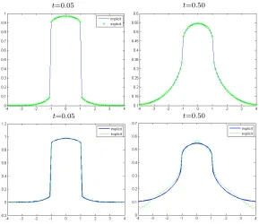
t=0.05 t=0.50

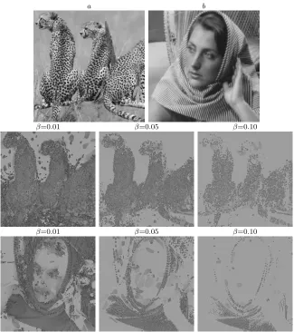
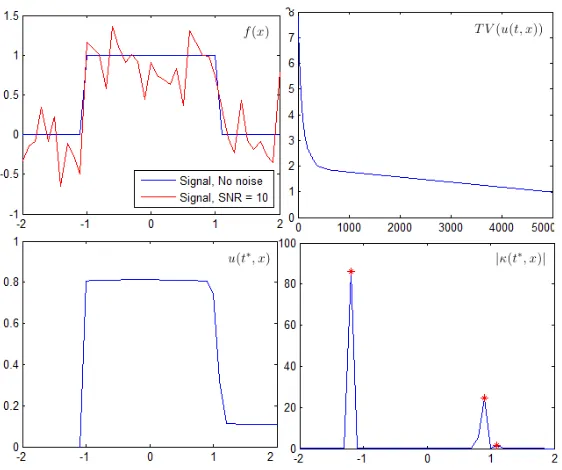
Figure 2.4: In this experiment, we use explicit and implicit difference schemes for 1D TV flow diffusion, with the initial condition x = −4 : 0.1 : 4,∆x = 0.1, f(x) = 1,|x| ≤

1; 0, else, = 0.1, in the four plots, explicit and implicit results are green and blue curves respectively. In the first row, ∆t= 0.25∆x2 satisfying the stability condition, we can see that the evolving results are very close between these two schemes; while in the second row, ∆t=∆x2 disobeys the stability condition, we can find for the explicit scheme, there are high oscillations, and implicit schemes are stable compared to both the explicit scheme and the first row.

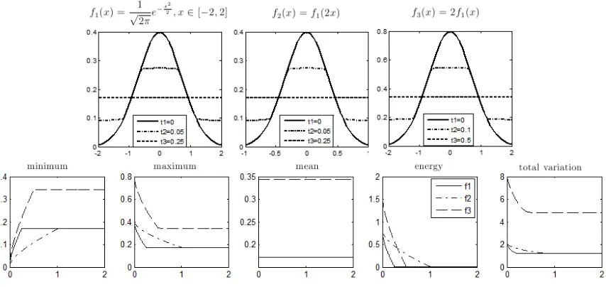
1D Signal Diffusion

Diffusion for 1D signal can be formulated in a general form:

∂u

(43)

Figure 2.5: Heat diffusion for three types of 1D signal(i.e. a(t, x) = 1)

2D image diffusion

For 2D images, we are interested to study effects of diffusion along local directions

ξ, η (may not necessarily be the local tangential or normal directions),

∂u

∂t(t, x) =a(x, t, u)∂ξξu(x, t) +b(x, t)∂ηηu(x, t) (2.4.2)

We will start from the following diffusion process.

∂u

∂t =∂ξξu(x, t), u(0, x) =f(x), x∈Ω⊆R

2 _(2.4.3)

The ξ used in the numerical experiments are N and T. Recall that

uN N =

uxxu2y−2uxuyuxy +uyyu2x

|∇u|2 , uT T =

uxxu2x+ 2uxuyuxy +uyyu2y

|∇u|2

In the example, we will compare the effects of the two diffusion equations.

(1)∂u

∂t =uN N; (2) ∂u

(44)

Figure 2.6: Image diffusion along directionN, T

Remark 2.4.1. Equation (2) in above is the mean curvature diffusion discussed in the

previous section. Compare (1) with (2) in Figure 2.6, it can be observed that the

diffusion force enforced by uN N tends to diffuse the image intensity along the normal

direction N of the level set. This force tends to distort the edge information, as

observed in Figure 2.6(1), edge structures are distorted to be round corners instead.

The diffusion along tangential direction tends to diffuse the image intensity along this

direction only, shown in Figure 2.6(2). In Figure 2.6, there are still slight blurring of

edges along N direction. It can be explained by the fact that a regularization term

1/p2₊_|∇_u_|2 _{was used in the numerical implementation to avoid the singularity for}

1/|∇u| occurs as |∇u| →0.

Remark 2.4.2. From the two examples, it becomes clear that image diffusion that

is normally expressed using (x, y) coordinates can be better interpreted based on a

decomposition of diffusion operators, using a local coordinate system. In general, this

local coordinate system uses the natural tangential and normal vectors of the level

(45)

diffusion along tangential direction is preferred to the normal direction. This is the

reason why mean curvature diffusion, total variation flow attracts more interests in

(46)

Chapter 3 Scale: Linear Diffusion

3.1 What is scale?

In computer vision research, multi-scale analysis and texture analysis are two branches

of study that have overlaps and both attract researchers’ interests. In addition, there

are applications in medical image analysis using multi-scale analysis and texture

anal-ysis. For example, in [26], authors use multi-scale analysis for blood vessel detection

and drusen detection in retina fundus image analysis. In [27], texture features of

digital mammogram images are extracted for breast tumor study.

The two terms Scale and Texture haven been used widely in theory and

applica-tions, however, neither scale nor texture has a uniform definition across the research

community[28, 29]. It is important and natural that if a term needs to be studied

quantitatively, the term should be based on a well-founded definition.

(47)

texture is the description of geometric patterns within an image. For example, in

[30], authors define ”texture” as repetitive patterns within the image(though, may

not be true for most of natural images). It is important to give a definition for these

terms which are used repeatedly in the analysis, otherwise complicated features are

generated from natural images, which cannot be interpreted properly. In our study,

the focus is the term scale. Based on the established mathematical theory, we aim to

establish the definition for scale that has better geometric interpretations.

How to define the term Scale?

Proper definition of a term can be related and decided for the purpose of a certain

application. Considering the definition of scale, First, if scale is a term used to

describe the coarseness of an image, it can be any parameter monotonically changing.

For example,t, the time parameter used in the diffusion equation, is commonly treated

as a scale parameter. Given image f(x), the solution to the equation at time t is

denoted as{u(x, t)}t>0. However, in general, it is not easy to relatetto any geometric

measure, especially for a nonlinear diffusion equation. It can only be said that the

parameter t provides a general sense that, as t increases gradually(for example), the

image is smoothed or the details within the image are gradually removed. Second, if

scale is the term used in the definition of local scale, it would be natural to expect that

thisscale measure the height, width, length, etc. i.e. scale defined pixel-wisely should

have a direct geometric meaning. The usage of the first interpretation(coarseness)

(48)

second interpretation can be seen in the detection of interesting or dominate scale.

For example, Lindeberg [6], Lowe [7], it is defined as the local extreme of a certain

edge response functions. In order to study multi-scale analysis based on nonlinear

diffusion, we begin with spaces based on linear diffusion.

3.2 Review: Linear Scale space

3.2.1 History of multi-scale analysis

The idea of using multiple resolution or multiple scales in image analysis is motivated

by the underlying natural multi-level structures of images. The study of multi-scale

analysis based on diffusion equations can be traced back to the work of Witkin, 1983

[31]. However, the idea of multi-scale analysis in image analysis is not a completely

new idea. From the early days, the simplest, yet still challenging image analysis

task is edge detection. This task partly motivated the usage of multi-scale analysis.

Examples of these work, include 1) Rosenfeld and Thurston(1971) [32]. 2) Klinger

(1971) [33]. The author used the idea of quad tree. The image is recursively divided

into smaller regions with a ratio of 2. Given image with size 2N ×2N, N ∈ Z, and

defines a measure V to describe the gray level variation of the subregions. Denote

f0 ₌ _f, _{if at stage} _i, _{the image variation} _V₍_fi_{) is larger than certain threshold} _v_,

the image fi will be divided into smaller region into fi+1. The process will ends

(49)

can be treated as ”merge and split” image segmentation task. The detailed example

is explained in [33]. 3) In the work of Burt(1981) [34] and Crowley(1991)[35], they

both proposed the pyramid representation of images. Instead of dividing the image

into subregions, the pyramid representation of an image of size 2N ×2N, N ∈ Z is

based on certain method of sub-sampling and smoothing. Naturally, from level fi _to

fi+1_{, the image is represented at a coarser level. By representing the image in this}

way, the size of the image decreases exponentially. 4) Wavelet theory is also widely

used in multi-resolution analysis, including the work of Mallat et.al.[36, 37, 38].

3.2.2 Linear multi-scale space

In 1983, Witkin proposed the multi-scale study based on gaussian smoothing in [31].

The basic idea is to embed the given imagef(x) into a family of solutions{u(t, x)}t>0

to the heat diffusion equation, parameter t is considered as the descriptor for scale.

Given f(x), x∈Ω⊆RN _{as the original image, the solution to the heat equation is}

u(t, x) = G(t, x)? f(x), G(t, x) = 1 (4πt)N/2e

−P

x2

i/4t, t >0 (3.2.1)

When N = 1, the conventional representation of a gaussian kernel is

G(σ, x) = √1

2πσe

−x2

(50)

The kernel size σ is directly related to the neighborhood size of each pixel x, and

√

2t can be interpreted as the measure of neighborhood size. In order to construct

scale analysis in a systematic way, there is some research on axioms for

multi-scale spaces. In the work of Alvarez[19], the multi-multi-scale analysis based on the heat

diffusion is proven to satisfy one axiom system.

Gaussian kernel, Derivatives and Scale

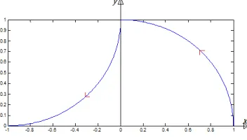
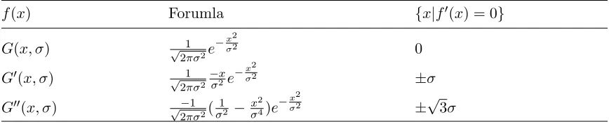
Figure 3.1 visualizes the property of gaussian kernel and its derivatives, and the

an-alytical results are summarized in Table 3.1.

Figure 3.1: Gaussian, Derivatives and Local Extreme Points

Table 3.1: Gaussian Kernel and Derivatives

f(x) Forumla {x|f0(x) = 0}

G(x, σ) √1

2πσ2e −x2

σ2 0

G0(x, σ) √1

2πσ2 −x

σ2e −x2

σ2 ±σ

G00(x, σ) √−1 2πσ2(

1 σ2 − x

2 σ4)e

−x2

(51)

3.2.3 Scale Selection

Construction of multi-scale space enables the analysis of a given image at different

scales, however what is more important is how to choose the proper scale for analysis.

Questions may include if local scale should be chosen adaptively for each pixel and

what criteria should be set up in order to select a meaningful scale. Compared to

literatures on multi-scale representation, there is less work on the discussion of scale

selection. One approach proposed by Schiele (1997) [39] is to use all information from

a range of different scales. This approach hugely increases the requirement of data

storage. Here, instead, we will mention the seminal work of Lindeberg(1993, 1994)

[6, 40], Lindeberg suggested the following principle for the automatic scale selection:

In the absence of other evidence, assume that a scale level, at which

some (possibly non-linear) combination of normalized derivatives assumes

a local maximum over scales, can be treated as reflecting a characteristic

length of a corresponding structure in the data.

3.2.4 Feature Detection: SIFT

One of the most important applications of the idea of scale selection is the scale

invariant feature transform(SIFT). It is a family of features that are invariant under

(52)

Lowe in 1999 [41], and then it is extended in a more systematic way in 2004 [7].

Lowe’s work provided a method to extract and describe distinctive and stable image

features that can be used in object recognition, object matching etc. Steps in feature

extraction can be divided into four main steps.

1, Scale-space extrema detection

In [41], the difference-of-Gaussian function(DOG) convolved with the image is used

to detect the stable key-point locations in the scale space. For 2D image,

L(x, y, σ) = G(x, y, σ)? f(x, y), G(x, y, σ) = 1 2πσ2e

−(x2₊_y2₎_/₂_σ2

D(x, y, σ) =L(x, y, kσ)−L(x, y, σ) (3.2.3)

The idea of DOG is shown in the left plot of Figure 3.2. Local extrema of D(x, y, σ)

Figure 3.2: Left: Calculation of DOG; Right: Key-point Localization

are detected by comparing the eight neighborhood points in the current image and

nine neighbors in the scale above and below. (x, y, σ) will be selected if D(x, y, σ) is

(53)

2, Key-point localization

Given the local extrema point (x, y, σ) in Step 1, the next step is to perform a detailed

fit to the nearby data for location, scale, and ratio of principal curvatures. This step

can reject points with low contrast, sensitive to noise etc.

G(v) =D((x, y, σ) +v) =D(x, y, σ) + ∂G

∂vv+

1 2v

T∂2G ∂v2v

The local extrema of G(v) is

ˆ

v =−∂

2_G

∂v

−1

∂G ∂v

ˆ

v is the offset with respect to (x, y, σ), if ˆv is larger than 0.5 in any dimension, the

sample point is changed and this step is performed again for the new sample point.

In addition, the response G(ˆv) is used to reject the unstable extrema point. In [41],

all extrema points with |G(ˆv)|<0.03 were discarded.

3, Orientation assignment

At each key point (x∗, y∗, σ∗) after Step 2, for each point (x, y) within the

neighbor-hood of the key-point,

m(x, y) =p(L(x+ 1, y)−L(x−1, y))2_{+ (}_L₍_{x, y}_{+ 1)}₋_L₍_{x, y}₋₁₎₎2

(54)

A histogram of θ(x, y) within this neighborhood(window size chosen to be 1.5σ) is

weighted by the gradient magnitude m(x, y). Peaks of this weighted histogram is

regarded as the dominant direction. The peak within 80% of the highest peak of the

histogram is used as the local orientation of the key-points.

4, Key-point descriptor

Key-point descriptor is composed of location (x, y), scale σ and local orientation θi.

Example

SIFT features have been used widely in image matching, feature analysis, since the

focus of our study is the image structure detection, it is better to start with analysis

on images containing simple shapes. In the following examples, we chose images with

typical blob(close to disk shape) and vessel(i.e. elongated shape) structures from both

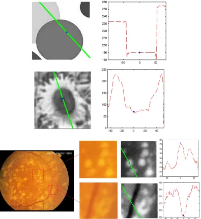
synthetic and real clinical images. Center of the yellow circle in the image indicates

the location of key-point (x, y) and the radius of the circle indicates the scale of the

key-point is denoted as σ.

(55)

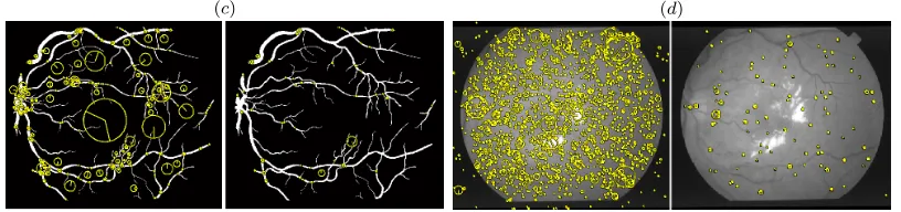
(c) (d)

Figure 3.3: Examples of SIFT Detection: For (b), (c), (d), Left figure: All key-points; Right figure: Randomly selected key-points

Remark 3.2.1. Based on Figure (3.3), it can be observed that (1) SIFT features works

best for blob detection, shown in (a). This can be partly explained by the fact that

heat diffusion is an isotropic diffusion; (2) For elongated structures, only points at

the two ends are detected, right figure of (a); In (c), junction points along the vessels

are detected. The fact that large part of edge structures is not detected can be

partly explained by the fact that heat diffusion is known to blur edge structures;

(3) The detection of scale can represent the relative relationship between scales of

structures shown in (a), (b), however in general, it is not absolutely correct; (4) In

(b), besides the bright blobs, the dark regions between blobs are also detected as

key-points. This can be explained by the fact that the blob detection was defined as

regions brighter or darker than the surrounding regions[42]. Additionally, there are

many small spots detected that may be due to the existence of oscillations within the

image. These oscillations can be removed by different choices of threshold(e.g. some

response function), however, in automatic image analysis, the choice of parameters

(56)

public dataset STARE for retina image analysis), the existence of many key-points

can pose a problem for additional key-point selection. The remarks we made here

do not mean that SIFT features are not helpful, but that the theoretical basis of

SIFT features can limit SIFT in some image analysis tasks, especially for elongated

structures(i.e. vessel structures). It is a motivation for the intensive research on

(57)

Chapter 4 Total Variation model

4.1 Total Variation Flow Minimization

4.1.1 Total Variation and Bounded Variation

Images are usually considered in Lp(Ω) space, here Ω ⊆ Rn, however Lp(Ω) spaces

fail to capture the local oscillatory patterns within images. With the introduction of

Sobolev space W1,1_{(Ω), the irregularities of images are also taken into consideration.}

One limitation is that W1,1(Ω) space does not allow edges within an image. In

computer vision, edges are considered crucial clues for object pattern recognition. In

between the Lp_{(Ω) and} _W1,1_{(Ω) spaces, there is one function space that can balance}

the regularity characterization and accept edge structures at the same time. This

(58)

Definition 4.1.1. Given u∈L1(Ω),Ω⊆Rn,

kukT V(Ω) : Z

Ω

|Du|= sup{

Z

Ω

u∇ ·(~g)dx :g~∈C₀1(Ω;Rn),|~g(x)|l2 ≤1,∀x∈Ω}

kukBV(Ω) :=kukL1(Ω)+kukT V(Ω)

BV(Ω) ={u∈L1(Ω) :kukBV(Ω) <∞}

Here, for convenience, kukT V(Ω) is also denoted as kDuk(Ω). The total variation

normk · kT V is a semi-norm; (BV(Ω),k · kBV(Ω)) is a Banach space. The introduction

of BV spaces in imaging processing is in the work of Rudin, Osher and Fatemi [20,

21].The relationship between BV space and the two function spaces mentioned before

can be summarized as the following:

W1,1(Ω)⊆BV(Ω) ⊆L1(Ω)

4.1.2 ROF Model

The total variation minimization model appeared in the seminal work of

Rudin-Osher-Fatemi [20]. The model proposed for the image denoising problem as the following:

given an observed image u0(x, y) =u(x, y) +n(x, y),(x, y) ∈ Ω,where n(x, y) is the

additive noise, and u(x, y) is the original image that needs to be reconstructed.

Dif-ferent from previous researches [43, 44, 45] in which the least squares criteria (i.e. L2

(59)

mini-mizing the total variation norm of the image. It has been suggested in [46] that the

total variation norm(i.e. TV norm) is a better norm to describe an image than theL2

norm, especially for images with edges as discontinuities. The optimization problem

is proposed with constraints shown as follows

min

u∈BV(Ω) Z

Ω q

u2

x+u2ydxdy

subject to

Z

Ω

u(x, y)dxdy=

Z

Ω

u0(x, y)dxdy,

Z

Ω

1

2(u−u0)

2

dxdy=σ2, σ >0.

This model is proposed with the prior information that the noise n(x, y) has zero

mean and standard deviation σ. In [20], this optimization problem is solved using

the gradient descent method.

∂u ∂t = ∂ ∂x( ux p u2 x+u2y

) + ∂

∂y( uy p

u2 x+u2y

) (4.1.1)

−λ(u−u0), t >0,(x, y)∈Ω (4.1.2)

u(x, y,0) is given (4.1.3)

∂u

∂n = 0 on∂Ω (4.1.4)

The model can also be reformulated as an equivalent unconstrained optimization

problem, commonly knows as ROF Model:

min

u∈BV(Ω)λ Z

Ω

|Du|+

Z

Ω

(60)

Here, λ > 0 is the weight between regularity and the fidelity term. The numerical

experiments in [20] demonstrate the ROF model (4.1.5) can perform best in denoising

very noisy images, especially yielding sharp edges in images. However, there is one

important limitation of (4.1.5) that is the loss of contrast in solutions, even when the

image f(x) is noise-free. Detailed discussions on the limitations of the ROF model

are shown in [47].

4.1.3 T V /L

1

Model

There have been many studies and variations of the ROF model (4.1.5), and T V /L1

is the model with special interests. In this model, the total variation norm is used in

the regularization term, and the fidelity term is replaced with L1 _{norm, the problem}

is proposed as (see [47]):

min

u∈BV(Ω)

λ

Z

Ω

|Du|+|f−u|_L1_(Ω) (4.1.6)

here f(x) is the image within region Ω⊆R2, Ω is a rectangle,|u|T V(Ω) is the

regular-ization term, |f−u|L1_(Ω) is the fidelity term, λ is the weight between regularity and

fidelity term. As λ increases, the minimizer of Problem (4.1.6) is a more regularized

version of the original image, and smaller feature including noise that has high

oscil-lation is gradually removed.

(61)

minimizer to Problem (4.1.6) is:

u(x, λ) =

              

k1Br(0)(x) λ <2r

{a1Br(0)(x)} λ= 2r,0< a < k,

0 λ >2r

(4.1.7)

In general, Problem (4.1.6) cannot be solved analytically and this simple example

demonstrates several important properties of T V /L1 model. First, the critical point

λ∗ = 2r at which the solution u(x, λ) changes from 0 to f depends on the radius of

the disk (i.e. the scale of geometric structure) only, and does not dependent on the

intensity level of the disk. It indicates thatT V /L1 model can maintain and reveal the

inherent geometric properties of the image. In image analysis, it is desired that image

structures be identified without any affects of the transformation of image intensity

values. Second, considering the solution to T V /L1, except at the point λ = 2r, the

solution is either 0 or f, and the general image contrast remains constant. On the

contrary, one of the known limitations of the ROF model is that the image contrast

will be decreased even for images without noise.

The effect of λ for ROF model and T V /L1 models are very different. For the ROF

model, objects of distinct scale with edges in the image gradually lose contrast and

merge with their neighbors as the parameter λ increases. In T V /L1 model, objects

can maintain their contrast with respect to their neighbors and their boundaries are

Study of Image Local Scale Structure Using Nonlinear Diffusion

University of Pennsylvania

ScholarlyCommons

Study of Image Local Scale Structure Using

Nonlinear Diffusion

Yan Wang

Study of Image Local Scale Structure Using Nonlinear Diffusion

STUDY OF IMAGE LOCAL SCALE STRUCTURE USING

NONLINEAR DIFFUSION

Acknowledgments

Contents

Chapter 1

Introduction

1.1

Motivation

1.2

Contribution

1.3

Organization

Chapter 2

Image Diffusion

2.1

Physical Background

2.2

Diffusion operator decomposition

2.2.1

Linear Diffusion: Heat Equation

2.2.2

Nonlinear Diffusion Equation

2.3

Numerical implementations

2.3.1

Linear Diffusion Equation

2.3.2

Nonlinear Diffusion

2.4

Interpretation of image diffusion

Chapter 3

Scale: Linear Diffusion

3.1

What is scale?

3.2

Review: Linear Scale space

3.2.1

History of multi-scale analysis

3.2.2

Linear multi-scale space

3.2.3

Scale Selection

3.2.4

Feature Detection: SIFT

Chapter 4

Total Variation model

4.1

Total Variation Flow Minimization

4.1.1

Total Variation and Bounded Variation

4.1.2

ROF Model

4.1.3

T V /L

Model