ScholarlyCommons
Publicly Accessible Penn Dissertations
Spring 5-17-2010
Sea-Level Changes Along the U.S. Atlantic Coast:
Implications for Glacial Isostatic Adjustment
Models and Current Rates of Sea-Level Change
Simon E. Engelhart
University of Pennsylvania, [email protected]
Follow this and additional works at:http://repository.upenn.edu/edissertations Part of theEarth Sciences Commons
This paper is posted at ScholarlyCommons.http://repository.upenn.edu/edissertations/407 Recommended Citation
Engelhart, Simon E., "Sea-Level Changes Along the U.S. Atlantic Coast: Implications for Glacial Isostatic Adjustment Models and Current Rates of Sea-Level Change" (2010).Publicly Accessible Penn Dissertations. 407.
Isostatic Adjustment Models and Current Rates of Sea-Level Change
Abstract
This study develops the first database of Holocene sea-level index points for the U.S. Atlantic coast using a standardized methodology. The database will help further understanding of the temporal and spatial
variability in relative sea-level (RSL) rise, provide constraints on geophysical models and document ongoing crustal movements due to Glacial Isostatic Adjustment (GIA). I sub-divided the U.S. Atlantic coast into 16 areas based on distance from the center of the Laurentide Ice Sheet. Rates of RSL change were highest during the early Holocene and have been decreasing over time, due to the continued relaxation response of the Earth’s mantle to GIA and the reduction of ice equivalent meltwater input around 7 ka. The maximum rate of RSL rise (c. 20 m since 8 ka) occurred in New Jersey and Delaware, which is subject to the greatest forebulge collapse. The rates of early Holocene (8 to 4 ka) rise were 3 - 5.5 mm a-1. I employed basal peat index points, which are subject to minimal compaction, to constrain models of GIA. I demonstrated that the current ICE-5G/6G VM5a models cannot provide a unique solution to the observations of RSL during the Holocene. I reduced the viscosity of the upper mantle by 50%, removing the discrepancy between the observations and predictions along the mid-Atlantic coastline. However, misfits still remain in Maine, northern Massachusetts and the Carolinas. Late Holocene (4 ka to present) RSL data are a proxy for crustal movements as the eustatic component was minimal during this time. Land subsidence is less than 0.8 mm a-1 in Maine, increasing to 1.7 mm a-1 in Delaware, and a return to rates lower than 0.9 mm a-1 in the Carolinas. This pattern results from the ongoing GIA due to the demise of the Laurentide Ice Sheet. I used these rates to remove the GIA component from tide gauge records to estimate a mean 20th century sea-level rise rate for the U.S. Atlantic coast of 1.8 ± 0.2 mm a-1. I identified a distinct spatial trend, increasing from Maine to South Carolina, which may be related to either the melting of the Greenland Ice Sheet, and/or ocean steric effects.
Degree Type
Dissertation
Degree Name
Doctor of Philosophy (PhD)
Graduate Group
Earth & Environmental Science
First Advisor
Benjamin P. Horton
Keywords
sea level, salt marsh, holocene, laurentide, climate, atlantic coast
Subject Categories
SEA-LEVEL CHANGES ALONG THE U.S. ATLANTIC
COAST: IMPLICATIONS FOR GLACIAL ISOSTATIC
ADJUSTMENT MODELS AND CURRENT RATES OF
SEA-LEVEL CHANGE
Simon E. Engelhart
A DISSERTATION
in
Earth and Environmental Science
Presented to the Faculties of the University of Pennsylvania
in
Partial Fulfillment of the Requirements for the
Degree of Doctor of Philosophy
2010
Supervisor of Dissertation
Dr. Benjamin P. Horton, Associate Professor, Earth and Environmental Science
Graduate Group Chairperson
Dr. Arthur H. Johnson, Professor, Earth and Environmental Science
Dissertation Committee
Adjustment Models and current rates of sea-level change
COPYRIGHT
2010
I would firstly like to thank my supervisor Ben Horton. Ben’s enthusiasm for
understanding sea-level changes inspired me to study the topic as an undergraduate
and continues to inspire me to this day. His encouragement, expertise, guidance and
friendship, made this dissertation possible. A special debt of thanks must also go to
Tor Törnqvist for his advice and constructive comments throughout my PhD. I would
also like to thank my co-authors Dick Peltier and Bruce Douglas, who have provided
invaluable advice and comments throughout the last five years.
I thank the entire faculty at the Department of Earth and Environmental Science,
particularly my committee members, Fred Scatena and Bob Giegengack. Joan and
Arlene have continually made my life easier providing administrative and organizational
support.
A large component of any study is the people with which you share the experience. I
would like to acknowledge the Sea-Level Research Laboratory, particularly Andrew
“Derby” Kemp, Andrea Hawkes, Christopher Bernhardt and Candace Grandpre for
Chuck Romanchock have been the best office mates you could ever wish to have.
I would like to acknowledge funding from the National Science Foundation, the
Earthwatch Foundation, a Geological Society of America graduate student grant, the
University of Pennsylvania Summer Stipend in Paleontology and research and teaching
fellowships from the University of Pennsylvania. I particularly want to acknowledge the
Thouron Family, who funded my first two years of graduate study.
Finally, I wish to thank my family, especially my Dad, whose emotional and financial
support has allowed me to be in this position today. My fiancée Lucy has been the firm
grounding on which this whole dissertation rests.
Finally, I am indebted to other researchers who have provided assistance throughout my
PhD years including Roland Gehrels, Antony Long, Glenn Milne, Orson van de Plassche,
SEA-LEVEL CHANGES ALONG THE US ATLANTIC COAST: IMPLICATIONS FOR GLACIAL ISOSTATIC ADJUSTMENT MODELS AND CURRENT RATES OF
SEA-LEVEL CHANGE
Simon E. Engelhart
Benjamin P. Horton
This study develops the first database of Holocene sea-level index points for the
U.S. Atlantic coast using a standardized methodology. The database will help further
understanding of the temporal and spatial variability in relative sea-level (RSL) rise,
provide constraints on geophysical models and document ongoing crustal movements
due to Glacial Isostatic Adjustment (GIA). I sub-divided the U.S. Atlantic coast into
16 areas based on distance from the center of the Laurentide Ice Sheet. Rates of RSL
change were highest during the early Holocene and have been decreasing over time, due
to the continued relaxation response of the Earth’s mantle to GIA and the reduction of ice
equivalent meltwater input around 7 ka. The maximum rate of RSL rise (c. 20 m since
8 ka) occurred in New Jersey and Delaware, which is subject to the greatest forebulge
collapse. The rates of early Holocene (8 to 4 ka) rise were 3 - 5.5 mm a-1. I employed
basal peat index points, which are subject to minimal compaction, to constrain models
of GIA. I demonstrated that the current ICE-5G/6G VM5a models cannot provide a
unique solution to the observations of RSL during the Holocene. I reduced the viscosity
of the upper mantle by 50%, removing the discrepancy between the observations and
northern Massachusetts and the Carolinas. Late Holocene (4 ka to present) RSL data are
a proxy for crustal movements as the eustatic component was minimal during this time.
Land subsidence is less than 0.8 mm a-1 in Maine, increasing to 1.7 mm a-1 in Delaware,
and a return to rates lower than 0.9 mm a-1 in the Carolinas. This pattern results from the
ongoing GIA due to the demise of the Laurentide Ice Sheet. I used these rates to remove
the GIA component from tide gauge records to estimate a mean 20th century sea-level rise
rate for the U.S. Atlantic coast of 1.8 ± 0.2 mm a-1. I identified a distinct spatial trend,
increasing from Maine to South Carolina, which may be related to either the melting of
Chapter One IntrOduCtIOn 1
Dedication iii
Acknowledgements iv
Abstract vi
List of Contents viii
List of Figures xiii
List of Tables xvi
1.1 Context 1
1.2 Thesis Aims 3
1.3 Thesis Structure 6
2.1 Introduction 8
2.2 Relative Sea Level 10
2.2.1 Eustasy 11
2.2.2 Isostasy 15
2.2.3 Tectonics 25
2.2.4 Local 25
2.3 Reconstructing Relative Sea Level 30
from the US Atlantic Coast
2.3.1 Sea-Level Index Points 30
reCOnstruCtIngLatequaternary
Chapter twO reLatIvesea LeveL: methOdOLOgIes 8
2.3.2 Chronological Issues in Relative
Sea-Level Reconstructions 35
2.4 Geophysical and Instrumental 38
Methods for Reconstructing Components of Relative Sea Level for the U.S. Atlantic Coast
2.4.1 GIA Models 38
2.4.2 Tide Gauges 42
2.4.3 Satellite Altimetry 45
2.4.4 Gravity 48
2.4.5 Global Positioning Systems 51
2.5 Geology and Geomorphology of 52
the U.S. Atlantic Coast
2.5.1 Maine 54
2.5.2 Massachusetts 54
2.5.3 Connecticut 55
2.5.4 New York 56
2.5.5 New Jersey 57
2.5.6 Delaware 57
2.5.7 Maryland and Viginia 58
2.5.8 North Carolina 59
2.5.9 South Carolina 59
2.6 Summary 60
3.1 Abstract 63
3.2 Introduction 65
3.3 The U.S. Atlantic Coast 67
Chapter three hOLOCene reLatIve sea LeveLsOfthe 63
3.4.1 Example of a Late Holocene Basal 77
Sea-Level Index Point from New Jersey
3.5 Holocene Relative Sea-Level History 80
of the U.S. Atlantic Coast
3.5.1 Northeastern Atlantic Region 82
3.5.2 Mid-Atlantic Region 84
3.5.3 Southern Atlantic Region 87
3.6 Discussion 89
3.6.1 Holocene RSL History of the U.S. 89
Atlantic Coast
3.6.2 Data Resolution and Spatial Area 93
3.7 Conclusions 96
4.1 Abstract 98
4.2 Introduction 100
4.3 Methods 102
4.3.1 Geological Data 102
4.3.2 Model Data 104
4.4 Results 104
4.5 Discussion 108
4.6 Conclusions 110
Chapter fOur hOLOCene reLatIve sea LeveLsOfthe
u.s. atLantIC COast: ImpLICatIOns fOr 98
gLaCIaL IsOstatIC adjustment mOdeLs
spatIaL varIabILIty Of Late hOLOCeneand
Chapter fIve 20th Century sea-LeveL rIse aLOngthe 112
5.1 Abstract 112
5.2 Introduction 114
5.3 Methodology 115
5.3.1 Construction of a Sea-Level Index Point 115
5.3.2 Geological Records 116
5.3.3 Tide Gauge Records 117
5.4 Analysis 117
5.5 Discussion 122
5.6 Supplementary Materials 126
5.6.1 Supplementary Information A: 126
Sea-Level Index Points
5.6.2 Supplementary Information B: Late 129
Holocene Rates of Relative Sea-Level Rise
5.6.3 Supplementary Information C: Uncertainty 135
of Sea-Level Trends from Tide Gauge Data
6.1 Holocene Relative Sea Levels of the 138
Atlantic Coast of the United States
6.2 Holocene Relative Sea Levels of the 141
U.S. Atlantic Coast: Implications for Glacial Isostatic Adjustment Models
6.3 Spatial Variability of Late Holocene and 143 20th Century Sea-Level Rise along the
Atlantic Coast of the United States
6.4 Areas of Future Research 146
6.4.1 Tidal Modeling 146
Dated Index Points
6.4.4 Spatial and Temporal Data Distribution 148
6.4.5 Geophysical Modeling 149
6.4.6 Fingerprints of Glacial Melting 149
6.4.7 Assimilation with the Gulf Coast and 150
Caribbean Databases
appendIx 151
referenCes 162
L
Ist Off
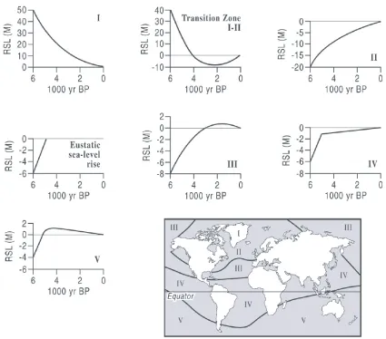
IguresFigure 2.1 Distribution of regional sea-level zones and 12 typical relative sea-level curves
Figure 2.2 Sea-level changes in response to the collapse 14 of the western Antarctic ice sheet
Figure 2.3 Relative sea-level curves for four locations in 17 southern Greenland
Figure 2.4 Observations and model predictions of relative 18 sea-level change 16 ka to present from Arisaig,
Scotland
Figure 2.5 Updated relative local sea-level curve for 20 Delaware
Figure 2.6 A schematic illustrating the two physical 21 mechanisms that dominate late Holocene
sea-level change in far-field locations
Figure 2.7 Sea-level curve for the Sunda Shelf derived 23 from shoreline facies
Figure 2.8 Zones in which the RSL predictions lie within 24 1 m of the mean eustatic value at 6 ka
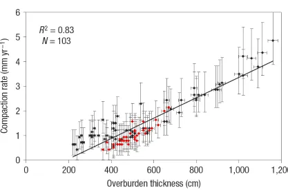
Figure 2.9 Relationship between overburden thickness 27 and compaction rate
Figure 2.10 Schematic representation of the Indicative 32 Meaning
Figure 2.11 Laurentide ice sheet topography in ICE-4G 41 and ICE-5G
tide gauges
Figure 2.13 Altimeter MSL from JASON-1 and TOPEX/ 47 Poseidon over the 1993-2007 period
Figure 2.14 Ocean mass change from GRACE over 50 2003-2008
Figure 3.1 Location map of the U.S. Atlantic coast showing 67 the study area from Maine to South Carolina
Figure 3.2 Location of the New Jersey study site within 78 the United States of America
Figure 3.3 Sea-level index points for 16 areas along the 83 U.S. Atlantic coast plotted as calibrated age
versus relative sea level
Figure 3.4 Sea-level index points for the16 areas along 85 the U.S. Atlantic Coast
Figure 3.5 Sea-level index points for the16 areas along 88 the U.S. Atlantic Coast
Figure 3.6 Rates of relative sea-level rise for the last 4 ka 90 plotted against the last 2 ka
Figure 3.7 Summary curves for the 16 areas along the 92 U.S. Atlantic Coast
Figure 4.1 Age-altitude plots of RSL observations and 105 model predictions for 16 different areas from
Maine to South Carolina on the U.S. Atlantic coast.
Chapter three
Figure 5.1 Rate of late Holocene relative sea-level rise 118 with two sigma errors for 19 locations along the
U.S. Atlantic coast
Figure 5.2 Detrending of 20th century tide gauge relative 121 sea-level rise (RSLR) with rates of late Holocene
relative sea-level rise for 10 locations along the US Atlantic coast
Figure 5.3 Rate of late Holocene relative sea-level rise with 123 two sigma errors for 19 locations along the U.S.
Atlantic coast
Figure 5.4 All 212 radiocarbon dated basal index points, 130 covering the last 4 ka
Figure 5.5 6 locations along the U.S. Atlantic Coast with 131 three or more basal sea-level index points and
the late Holocene rates of RSL rise
Figure 5.6 6 locations along the U.S. Atlantic Coast with 132 three or more basal sea-level index points and
the late Holocene rates of RSL rise
Figure 5.7 6 locations along the U.S. Atlantic Coast with 133 three or more basal sea-level index points and
the late Holocene rates of RSL rise
Figure 5.8 Eastern shore of Virginia with three or more 134 basal sea-level index points and the late
Holocene rates of RSL rise
Figure 5.9 Long-term tide gauge records from Canada 137 to Virginia, USA, plotted against distance from
Churchill, Canada
Table 3.1 Indicative meanings for the different sample 72 types within the database.
Table 3.2 Individual error terms that are considered for 74 each sample and contribute to the total error term.
Table 3.3 A summary of the RSL data for the 16 areas with 81 GPS coordinates shown.
Table 5.1 Location of the 19 sites along the U.S. Atlantic 120 Coast and the rate of late Holocene (last 4 ka)
relative sea-level rise (RSLR) derived from geological data.
Chapter fIve
IntroductIon
1.1 context
International Geoscience Programme 495 (Quaternary Land – Ocean Interactions:
Driving Mechanisms and Coastal Responses) seeks to understand the relative sea-level (RSL) changes since the Last Glacial Maximum (LGM). This aim can only be achieved
if reliable reconstructions of RSL from around the globe are available. The U.S. Atlantic
coast has a wealth of RSL research, commencing in the 1960s (e.g. Stuiver and Daddario,
1963; Bloom, 1963; Kaye and Barghoorn, 1964: Redfield, 1967; Belknap and Kraft,
1977; Field et al., 1979; Cinquemani et al., 1982; Pardi et al., 1984; van de Plassche,
1989; Gehrels and Belknap, 1993; Fletcher et al., 1993; Kelley et al., 1995; Barnhardt
et al., 1995; Nikitina et al, 2000; Miller et al., 2009; Kemp et al., 2009) but the data has
never been critically validated to ensure its accuracy.
To address this significant gap in our understanding, my research follows the consistent
methodology developed by the IGCP projects such as 61 and 200 (e.g. Cinquemani et
al., 1982; Greensmith and Tooley, 1982; Shennan, 1987) to produce validated records of
Holocene RSL for the U.S. Atlantic coast from (un)published radiocarbon dated
sea-level data. The U.S. Atlantic coast is important as it contains both near-field (formerly
ice covered) and intermediate-field (within the peripheral forebulge) sites, resulting in
spatially variable RSL histories during the Holocne due to the different interplay of the
eustatic and isostatic parameters (e.g. Clark et al., 1978; Lambeck, 1993; Milne et al.,
2005).
Sites from the U.S. Atlantic coast constitute vital constraints upon the dynamical models
of the Glacial Isostatic Adjustment (GIA) process (e.g. Peltier, 1996). GIA models
have been used to understand the rheology of the earth (e.g. Peltier, 1996; Davis and
Mitrovica, 1996; Shennan et al, 2002; Lambeck et al., 2004; Vink et al., 2007) and
constrain ice equivalent meltwater input (Milne et al., 2002, 2005; Bassett et al., 2005;
Peltier et al., 2005). Further, GIA models have been employed to filter tide gauge (e.g.
Tushingham and Peltier, 1989; Peltier, 1996; Davis and Mitrovica, 1996) and satellite
(Velicogna and Wahr, 2005, 2006; Velicogna, 2009) records of secular sea-level change
so as to isolate the contribution to this signal due to climate warming. There is an urgent
need for a sufficiently accurate model of the GIA process to inform the global data set
currently being produced on the time dependence of the gravitational field of the planet
by the Gravity Recovery and Climate Experiment (GRACE) (Cazenave et al., 2009).
Geodetic constraints may be placed on GIA models by satellite techniques (e.g. Argus et
al., 1999; Snay et al., 2007), but they lack the vertical precision of established geological
methods (e.g. Shennan, 1989; Shennan and Horton, 2002) and cannot reconstruct changes
1.2 thesIs aIms
This thesis addresses three complementary aims with associated research questions:
1) To establish a quality controlled sea-level database from the Atlantic coast of the
United States for the Holocene (11.7 ka to present).
There is an urgent need for a re-assessment of the quality of the observational evidence of
former sea levels from the Atlantic coast of the United States, as well as concepts inherent
in the interpretation of data. Previous research has failed to meet the fundamental
criteria to produce an accurate sea-level database (Donnelly, 1998). This is important,
as the rates of sea-level rise obtained during this period represent the fundamental basis
for comparison with the historical and present day changes. Different types of
sea-level indicators have different degrees of precision, but this is often not acknowledged
(Zerbini, 2000) and common errors inherent to sea-level research are rarely quantified
(e.g. Shennan, 1986).
The research questions are:
1. Can the previous sea-level research along the U.S. Atlantic coast meet the validation
criteria to produce a sea-level index point?
3. Is there spatial heterogeneity within the observations of former RSL along the U.S.
Atlantic coast, and if so, what is driving this variability?
4. Has RSL risen above present during the last 6 ka?
5. Can the temporal variation in the ice equivalent meltwater input be identified?
6. Can the effects of local processes such as compaction be isolated from the index
points?
2) Apply the database to improve the accuracy of models of the GIA process along
the U.S. Atlantic coast.
Models of the GIA process are currently employed to filter tide gauge (e.g. Peltier, 1996;
Davis et al., 2008) and satellite (e.g. Velicogna and Wahr, 2005, 2006; Wahr, 2006;
Velicogna, 2009) records of secular sea-level change so as to isolate the contribution to
this signal due to climate warming. There is a need for a sufficiently accurate model of
the GIA process, as the results from the GRACE mission are highly dependent on the
removal of GIA trends to estimate increases in ocean volume (Cazenave et al., 2009).
Whilst the current generation model (ICE-5G VM5a) provides an accurate fit to the
observations from regions once covered by the Laurentide Ice Sheet (e.g. Hudson Bay), it
is currently unknown whether this holds true for sites within the periphery of the ice sheet
along the U.S. Atlantic coast. This is an independent test of the GIA model, as the data
The research questions are:
1. Can the current generation GIA model (ICE-5G VM5a) accurately predict the
observations of Holocene RSLs from the U.S. Atlantic coast?
2. If a misfit between the model predictions and the observations is observed, is it
systematic?
3. Can modifications to the earth and/or ice models reconcile any of the variance
between observations and predictions?
3) Document current crustal motions of the U.S. Atlantic coast as a tool to further
understand 20th century sea-level rise.
Background rates of RSL change in the late Holocene (4 ka to present) provide the
baseline that changes in the 20th and 21st centuries must be superimposed upon (e.g.
Velicogna and Wahr, 2006; Church and White, 2006; Rahmstorf et al., 2007; Jevrejeva
et al., 2008). Late Holocene rates provide a regional perspective on spatial variability
in RSL rise (e.g. Milne et al., 2009; Gehrels et al., in press). Crustal movements can
be estimated from late Holocene RSL data as the ice equivalent meltwater input was
zero or minimal, there are minimal tectonic effects on a passive margin and compaction
can be reduced by utilizing basal peat. A comparison may be made between the crustal
movements estimated by geological methods and global positioning systems.
1. What are the late Holocene crustal motions associated with the removal of the
Laurentide Ice Sheet?
2. Do the estimates of crustal motion have a spatial pattern along the U.S. Atlantic coast?
3. How do late Holocene rates compare with estimates from GPS observations?
4. Does the 20th century record of sea-level rise from the U.S. Atlantic coast exhibit
spatial variability?
1.3 thesIs structure
Chapter Two presents the scientific justification related to this research and associated
background information. An overview of sea-level data since the LGM is provided
to place this study into context. The methodology and terminology of reconstructing
observations of Holocene RSL is outlined and compared to alternative methods of
estimating RSL. These include GIA models, tide gauges, satellite altimetry, gravity
measurments and global positioning systems.
Chapter Three describes the development of the U.S. Atlantic coast RSL database.
The chapter aims to document the current state of knowledge concerning the RSL history
of the U.S. Atlantic coast by validating published and unpublished radiocarbon dated
are discussed. The chapter provides a discussion of the advantages and limitations of the
database. This paper is to be submitted to Quaternary Science Reviews.
Chapter Four demonstrates the application of observations of former RSL in
constraining models of the GIA process. This chapter compares the database of Holocene
RSL to the current state of the art GIA model of Dick Peltier (University of Toronto).
Observed misfits between the model predictions and data are investigated and refined ice
and earth models are presented. Further potential refinements are suggested which may
lead to greater improvement in the variance between observed and modeled RSL. I will
submit the publication to Geophysical Research Letters.
Chapter Five investigates the rates of glacial isostatic adjustment during the last 4 ka.
Basal salt marsh peat from Maine to South Carolina is used as a proxy for the continuing
glacial isostatic adjustment. The GIA observations are removed from 20th century tide
gauge records to understand the acceleration in sea-level rise during this time period and
to investigate spatial variability. This study has been accepted for publication in Geology
on the 1st December 2009.
Chapter Six summarizes the main conclusions drawn from this research and makes
reconstructing Late Quaternary relative sea Level:
methodologies and observations
2.1 IntroductIon
Observations of relative sea level (RSL) during the late Quaternary are significant to a
number of disciplines in the Earth sciences (e.g. Alley et al., 2005; Rohling, 2008; Siddall
et al., 2009). RSL data can be employed to provide information on the rheology of the
Earth (Shennan et al., 2002; Lambeck et al., 2004; Peltier, 2004; Horton et al., 2005;
Lambeck and Purcell, 2005; Milne et al., 2005; Vink et al., 2007; Brooks et al., 2008) and
ice sheet reconstructions, including sources of meltwater input (Milne et al., 2002; Peltier
and Fairbanks, 2006). Observations provide information on coastal evolution (e.g. Kraft,
1971; McLean, 1984; Barrie and Conway, 2002: Waller and Long, 2003; Behre, 2004;
Massey and Taylor, 2007), as sea level serves as the base level for continental denudation
(Summerfield, 1991). This further drives our understanding of the links between coastal
processes and human development (e.g. Stanley, 1998; Richardson et al., 2005; Day et
al., 2007; Turney et al, 2007).
The Database approach of reconstructing RSL since the Last Glacial Maximum (LGM)
has been successful for the UK (e.g. Shennan, 1989; Shennan and Horton, 2002;
Caribbean (Toscano and Macintyre, 2003; Milne et al., 2005), South America (Rostami
et al., 2000; Milne et al., 2005; Angulo et al., 2006), Southeast Asia (Horton et al., 2005;
Woodroffe and Horton, 2005), China (Zong et al., 2004) and Australia (e.g. Larcombe,
1995) . These databases have been used to calibrate models of earth rheology (e.g. Peltier
et al., 2002; Vink et al., 2007), constrain the source and magnitude of ice equivalent
meltwater input (e.g. Shennan et al., 2002; Bassett et al., 2005; Milne et al., 2005);
investigate the effects of sediment loading and compaction (e.g. Horton and Shennan,
2009), understanding the effects of tidal range change (e.g. Shennan et al., 2000; 2003),
producing baseline rates of RSL rise to compare with 20th century rates (e.g. Shennan and
Horton, 2002; Shennan et al., 2009) and constraining instrumental observations of crustal
movements (e.g. Teferle et al., 2009).
While there have been previous attempts to produce a database for the U.S. Atlantic
coast (e.g. Bloom, 1967; Newman et al., 1980, 1987; Cinquemani et al., 1982; Pardi
and Newman, 1987; Gornitz and Seeber, 1990; Tushingham and Peltier, 1992; Peltier,
1996; Donnelly, 1998) the fundamental criteria to produce an accurate sea-level database
have not been met. To address this I have collected over 50 fields of information for
each sample within the U.S. Atlantic coast database to enable me to validate samples as
sea-level index points. These include both data obtained from the authors (e.g. location,
lab code, radiocarbon age plus error) as well as calculations and interpretations made
error). Conditional filters can be applied to these fields, such as possible contamination
and stratigraphic context, to define those index points that I believe, from the published
information, to be reliably related to past tide levels.
This chapter introduces the methodology and terminology used when reconstructing RSL
in the U.S. Atlantic coast database. I provide a description of the four components that
combine to produce the RSL history at any point on the globe and describe the different
forms of RSL curves that are seen depending on the proximity to ice loading during the
LGM. I outline the requirements for a sample to be validated as a sea-level index point
and discuss potential errors induced when reconstructing RSL, including compaction,
tidal range and chronology. Modern instrumental methods for reconstructing components
of RSL and GIA modeling are discussed. Finally, I discuss the geological and
geomorphological setting of my study area; the U.S. Atlantic coast.
2.2 reLatIve sea LeveL
The processes that interact to produce a RSL curve at any one location on the surface of
the Earth is commonly described by the following equation (Shennan, 2009):
where τ and ψ represent time and space. Δξeus(τ)is the time-dependent eustatic function,
Δξiso(τ,ψ)is the total isostatic effect of the glacial rebound process including both the ice
(glacio-isostatic) and water (hydro-isostatic) load contributions, Δξtect(τ,ψ) is any tectonic
effects, while Δξlocal(τ,ψ) represents the local process involved (Shennan and Horton,
2002). Δξerror(τ,ψ) is unknown but we attempt to minimize this component by employing
proven methodologies.
2.2.1 Eustasy
The concept of eustasy was proposed by Eduard Seuss in 1888 to reflect global changes
in sea level due to the changing ratio between water stored in the oceans and water stored
on the continents as ice. This principle focused on the belief that any meltwater input
to the oceans would be evenly distributed over the entire globe. With the development
of radiocarbon dating (Libby, 1952) there was an increase in the collection of RSL
data as scientists sought to identify the ‘global eustatic curve’ (e.g. Fairbridge, 1961).
The development of geophysical models of RSL (e.g. Peltier et al., 1974, Farrell and
Clark, 1976; Clark et al., 1978) and the understanding that gravitational effects were an
important control on RSL (e.g. Clark and Lingle, 1977; Clark et al., 1978) highlighted
that a global eustatic curve could not exist (Figure 2.1). Analysis of RSL data confirmed
that the eustatic curve was an immeasurable factor at any one point on Earth (Kidson,
1986) and that it could only ever be inferred from sea-level data at multiple locations (e.g.
Research has demonstrated that while the ice equivalent meltwater input has only a
temporal component, changes in the gravitational attraction of melting and accreting
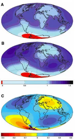
ice sheets (e.g. Clark and Lingle, 1977) and rotational changes (e.g. Mörner, 1976), can
result in spatially variable response to ice equivalent meltwater input, termed geoidal
eustasy. Therefore, the ocean surface cannot be considered as a flat surface, but one with
topography. This theory has been applied to ‘fingerprint’ the sources of meltwater input
during the 20th century (e.g. Conrad and Hager, 1997; Mitrovica et al., 2001; Tamisiea
et al., 2001) and to predict the effects of future melting scenarios (e.g. Mitrovica et al.,
2009) (Figure 2.2).
The eustatic minimum coincides with the last glacial maximum (LGM), previously
considered to be between 24 - 21 ka (Aharon, 1984; Fairbanks, 1989; Bard et al., 1990a,
b; Pirazzoli, 1996; Fleming et al., 1998; Yokoyama et al., 2001; Clark and Mix, 2002;
Peltier, 2002; Bird et al., 2005; Murray-Wallace, 2007; De Deckker and Yokoyama,
2009) when as much as 50 million km3 of ice was transferred between the oceans and
continents (e.g. Fleming et al., 1997; Yokoyama et al., 2000; Lambeck et al., 2002).
However, there is conflicting evidence from an updated Barbados record that suggests
that this should be 26 ka with 21 ka marking the commencement of deglaciation (Peltier
and Fairbanks, 2006). Further, there is controversy surrounding the eustatic minimum
et al., 2000; Peltier and Fairbanks, 2006). From deglaciation RSL rise proceeded at c. 6
mm a-1 (Fleming et al., 1998) before an increase to rates of c. 10 mm a-1 between 17 – 7
ka (Fleming et al., 1998). However, this rate was not constant but exhibited departures
termed ‘meltwater pulses’ of up to 40 mm a-1 (Fairbanks, 1989, Alley et al., 2005; Peltier
and Fairbanks, 2006). The sources of these meltwater pulses remain contentious. Peltier
(2005) favors a Laurentian source for meltwater pulse 1a (c. 14.5 ka) whereas Clark et al.
(2002) and Bassett et al. (2005) suggest that variability between models and observations
during this time can be reduced with an Antarctic source. There is further controversy
surrounding the termination of eustatic input during the late Holocene. Peltier (1998,
2002) proposes that meltwater input ceased c. 4 ka, whereas other research groups allow
either 0.1 - 0.2 mm a-1 melting from 4 ka to 2 ka (e.g. Lambeck, 2002) or propose a
scenario with continued melting to 1 ka (Fleming et al., 1998).
2.2.2 Isostasy
The first known documentation of postglacial land uplift is dated to A.D. 1491, when the
inhabitants of the Swedish town of Östhammar reported that fishing boats could no longer
reach the town “due to a growth of the land at the sea” (Ekman, 1991). The influence
of istostasy on RSL histories was further understood from the depression of the surface
of the earth by large continental ice sheets at the LGM. The response to this loading
continues to the present day (e.g. Walcott 1972, Peltier et al., 1978). Therefore, different
and far-field regions (e.g. Clark et al., 1978). Near-field (e.g. Greenland, Canada,
Northwest Scotland) regions are or were previously underneath ice masses, which caused
the solid earth to subside. Following deglaciation, the solid earth uplifts as it regains
isostatic equilibrium. At southern Greenland, the ice load was > 1.5 km thick (Bennike
and Bjorck, 2002). As the depressed crust starts to uplift, RSL falls monotonically from
the LGM to 2 ka (Long et al. 2003) (Figure 2.3). Long et al. (2003) demonstrated that
the fall in RSL commenced from 108 m at 10.6 – 10.2 ka until it intersected present sea
level at 3.5 ka. At 1.8 ka, RSL started to rise at c. 2 mm a-1 to the present. This rise is
associated with the neoglaciation of Greenland, which caused the region to subside. In
regions with thinner ice load (e.g. Arisaig, Scotland, < 1 km (Shennan et al., 2006)) the
RSL curve can be distinctly non-monotonic. Shennan et al. (2005) showed an initial
fall in RSL after the LGM due to rapid isostatic uplift (Figure 2.4). In the early to mid
Holocene the isostatic process subsides to less than the eustatic input, resulting in a
slight RSL rise. The declining eustatic function after 6 ka causes a further switch as RSL
history is dominated by the continuing low rate of isostatic uplift.
Intemediate-field regions (e.g. southeast England, France, Delaware) are found at the
periphery of the ice sheet where a forebulge is present due to the displacement of mantle
material from near-field regions (e.g. Wu and Peltier, 1983). Therefore, areas within the
periphery of the ice sheet were at a higher elevation with respect to the geoid at the LGM
the peripheral forebulge resulting in subsidence. As glaciation was a stepwise process
and did not occur instantly, the movement of the mantle material varies over time and
results in unique RSL curves at different intermediate-field areas (e.g. Tushingham and
Peltier, 1992). RSL rise is expected to slow due to the exponential form of the forebulge
collapse (e.g. Wu and Peltier, 1983).
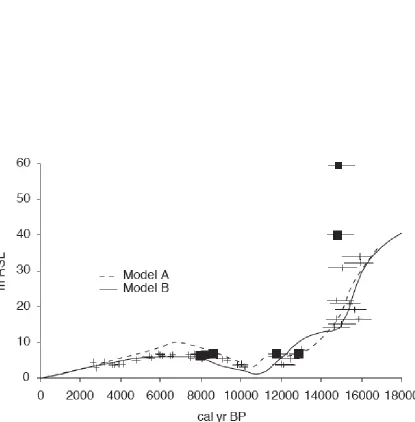
Nikitina et al. (2000) presented a late Glacial RSL record (Figure 2.5) from the inner
and outer Delaware estuary; an intermediate-field site. The record is well constrained by
sea-level data from 7 ka to present. RSL rose at a decreasing rate through the mid and
late Holocene. RSL rise decreased from 3.0 ± 0.2 mm a-1 from 7 – 5 ka, to 1.9 ± 0.1 mm
a-1 from 4 – 1.25 ka. A further reduction is seen from 1.25 ka to present to 0.9 ± 0.07 mm
a-1.
Far-field areas are not directly affected by the ice loading or the peripheral forebulge. In
these areas the effects of hydro-isostasy become dominant (e.g. Milne and Mitrovica,
2002). These effects consist of the subsidence of the oceanic crust due to water loading
(e.g. Peltier et al., 2009), the levering effect of a reduced sea-level position on the edge of
the continental shelf (e.g. Mitrovica and Milne, 2002) (Figure 2.6) and the movement of
water to occupy areas of forebulge collapse within the ocean (equatorial ocean siphoning;
Far-field sites have commonly been chosen as locations for RSL reconstructions
since deglaciation, as it was believed that this offered the opportunity to minimize
contamination from the effects of isostasy and focus solely on the eustatic component.
Records have been produced from a variety of sea-level indicators (e.g. corals,
foraminifera) from the Sunda Shelf (Hanebuth et al., 2000), Tahiti (Bard et al., 1996;
Montaggioni et al., 1997), the Huon Peninsula (Chappell, 1974; Chappell and Polach,
1991; Chappell et al., 1996), Australia (Thom and Chappell, 1975; Thom and Roy, 1985;
Yokoyama et al., 2000) and the classic records from Barbados (Fairbanks 1989, Bard
et al., 1990a, b; Peltier and Fairbanks, 2006). Hanebuth et al. (2000) presented a RSL
record from 21 – 10 ka for the Sunda Shelf (Figure 2.7). The reconstruction is based
on sediments from a delta plain, including mangrove and tidal flat deposits. The RSL
data fills the gap from 21 – 14 ka, where there was previously a shortage of RSL data.
Furthermore, it confirms the reconstructions of far-field sea level based on coral data.
An initial slow rise in RSL from the termination of the LGM at 21 ka, is punctuated by a
rapid increase of 16 m within 300 a (14.6 – 14.3 ka). This has previously been identified
from the Barbados record (Fairbanks, 1989) and is termed meltwater pulse 1A.
However, recent research has suggestedthat many of these studies are not from areas
ideal for inferring the eustatic signal (Milne and Mitrovica, 2008), due to sensitivity to
ice model or mantle viscosity choices. Therefore, GIA models can guide field scientists
at different points in time to test the current eustatic models (Figure 2.8) (Milne and
Mitrovica, 2008).
2.2.3 tEctonIcs
One-third of the Earth’s coastal margins lie along or near tectonically active plate
boundaries (Nelson, 2007). Both geological (e.g. Atwater, 1989; Long and Shennan,
1994; Nelson et al., 1996) and instrumental (e.g. Pirazzoli, 1996; Scholz, 2002; Ota and
Yamaguchi, 2004) methods have been applied to understand the patterns of deformation
associated with active margins. Indeed, far-field records used to constrain the ice
equivalent meltwater input including Barbados (e.g. Fairbanks, 1989), Tahiti (e.g. Bard
et al., 1996) and Papua New Guinea (e.g. Chappell and Polach, 1991) must be corrected
for the role of tectonics since the LGM. However, tectonic effects are considered to be
negligible on passive margins such as the U.S. Atlantic coast during the late Quaternary
(e.g. Szabo, 1985). Evidence for neotectonic activity as an explanation for differing RSL
curves has also been rejected after careful consideration of the data (e.g. Gehrels and
Belknap, 1993; van de Plassche et al., 2002).
2.2.4 LocaL
The total effect of local process at a site can be expressed schematically (Shennan and
Δξlocal(τ,ψ) = Δξtide(τ,ψ) + Δξsed(τ,ψ)
whereΔξtide(τ,ψ) is the total effect of tidal regime changes and the elevation of the
sediment with reference to tide levels at the time of deposition, and Δξsed(τ,ψ) is the total
effect of sediment consolidation since the time of deposition.
The local effects on RSL are principally sediment compaction under its own and other
sediment package’s weight (e.g. Jelgersma, 1961; Kaye and Barghoorn, 1964) and
changes in tidal regime due to differing paleogeographies in the past (e.g. Scott and
Greenberg, 1983; Gehrels et al., 1995; Shennan et al., 2000, 2003). Sediment compaction
(or consolidation) is a result of the reduction of void space within the sedimentary
column (e.g. Greensmith and Tucker, 1986). Compaction will lower sea-level data from
the elevation at which they formed, resulting in erroneous reconstructions (Shennan,
1986). Compaction is a complex process involving many variables (Pizzuto and
Schwendt, 1997) such as the nature of the substrate and mass of overburden, which vary
in time and space (Jelgersma, 1961; Kaye and Barghoorn, 1964; Törnqvist et al., 2008).
The thickness of overburden has been shown to be a significant variable in data from the
Missisippi Delta (Figure 2.9), suggesting millennial scale compaction rates up to 5 mm a-1
(Törnqvist et al., 2008).
Skempton, 1970; Paul and Barras, 1998), the uncertainty associated with them has led
to them rarely being applied (Shennan and Horton, 2002). To attempt to remove this
error, base of basal peat have been used (e.g. Jelgersma, 1961; Kaye and Barghoorn,
1964; van de Plassche, 1979, 1982; Smith, 1985; Denys and Baeteman, 1995). These
materials are compaction free because the underlying Pleistocene sands are practically
unaffected by compaction (Jelgersma, 1961). However, there are a number of problems
with basal peats. Firstly, it is important to assess whether sea level or local groundwater
level is controlling formation. Kiden (1995) noted that data collected by Jelgersma
(1961) appeared to plot anomalously high on an age/altitude graph relative to sea-level
curves for the rest of the Netherlands. Van de Plassche (1979) concluded that basal peat
samples could only be employed in sea-level reconstructions after a detailed study of the
relief of the underlying Pleistocene sands. Samples should only be taken where there
was a sufficient slope in the Pleistocene surface to avoid this groundwater-gradient effect
(van de Plassche, 1979). Secondly, basal peats are rare and therefore any reconstructions
reliant solely upon these data are liable to have significant gaps in the record. Finally,
basal peats are often devoid of identifiable plant macrofossils or microfossils making it
difficult to assess the relationship between the sample and sea level.
Sea-level researchers have therefore sub-divided samples based on potential for
compaction, without assessing the absolute amount (e.g. Shennan et al., 2000). This
al., 2000). Samples identified as basal come from within the unit overlying the
uncompressible substrate but are not from the base of the unit and may be subject to some
degree of compaction (Horton and Shennan, 2009). Intercalated samples are organic
sediments underlain and overlain between different sedimentary units and are the most
prone to compaction (Shennan, 1989).
Tidal range changes are important to reconstructions of RSL, as the methodology
inherently assumes that tidal range has not varied through time (Shennan, 1980).
Shennan (1980) acknowledged that this assumption reduces the value of the sea
level indicators, but is necessary to allow for the use of sea-level data with different
relationships to tidal levels. Models have been produced to assess the effects of tidal
range change (e.g. Scott and Greenberg, 1983; Gehrels et al., 1995; Shennan et al., 2000;
Shennan et al., 2003). Tidal range changes may stem from long-term changes in the
tidal potential arising from variations in the orbital elements of the Sun and Moon, from
changes in the shape or depth of ocean basins and/or the rate of global tidal dissipation
(e.g. Woodworth et al., 1991). Various researchers have identifiedthat shelf width and
basin configuration (Redfield, 1958; Jardine, 1975; Cram, 1979; Woodworth et al., 1991)
strongly influence tidal range. Changes in these paleogeographies may be due to
long-term processes including RSL change, sediment supply and/or anthropogenic processes
including dredging (Woodworth et al., 1991). It has been demonstrated that the effects of
in the difference between mean tide level and mean high water spring tide of c 2.5 m in
the Humber between 6 - 3 ka (Shennan and Horton, 2002). Scott and Greenberg (1983)
used numerical modeling in the Bay of Fundy to infer a 1.2% increase in tidal range for
every 1 m of sea-level rise between 7 and 2.5 ka. Gehrels et al. (1995) focused on the M2
tidal component and demonstrated that it was 73% of the modern value at 5 ka. Changes
in tidal regime are currently beyond the scope of this study. However, the outputs from
this research will increase the accuracy of paleogeographic maps for a current study of
tidal range during the Holocene (David Hill, The Pennsylvania State University)
2.3 reconstructIng reLatIve sea LeveL from the u.s. atLantIc
coast
2.3.1 sEa-LEvEL IndEx PoInts
A sea-level index point is a datum that can be utilized to show vertical movements of sea
level. Index points as a concept were proposed and subsequently developed during the
International Geoscience Programme (IGCP) Projects 61 and 200 (e.g. Cinquemani et al,
1982; Shennan, 1987).
For a sample to be considered an index point it must have three components: (1) a
geographical location; (2) an altitude that can be related to a former water level; and (3)
GPS co-ordinates or identification from site maps then the sample cannot be considered a
valid index point.
A sample must possess a systematic and quantifiable relationship to a tide level, which
can be observed in the modern environment and, therefore, be used to estimate former sea
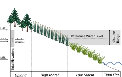
level. This is formalized through the concept of the indicative meaning (e.g. Shennan,
1986; van de Plassche, 1986). It contains two components, the indicative range (the
elevational range occupied by a sea-level indicator) and the reference water level (the
relation of that indicator to a contemporaneous tide level, e.g. mean high water (MHW)).
The reference water level does not have to be equal to a tide level, but can be offset (e.g.
MHW + 0.2 m), a term known as the indicative difference. However, Shennan, (1986)
stated that the reference water level should ideally be given as a mathematical expression
of tidal parameters rather than a single tide level ± a constant, as the constant factor will
indicate quite different tidal inundation characteristics for areas of different tidal range. A
schematic of the indicative meaning is shown in Figure 2.10.
Index points can be produced from a wide array of sedimentary environments and
geomorphic features where the relationship between the sample and a water level can
be reliably established. In this thesis these include plant macrofossils, microfossils and
geochemical data. Samples identified only as salt marsh in origin can be assigned an
(e.g. van de Plassche et al., 1998). The low marsh is dominated by Spartina alterniflora
(e.g. Gehrels, 1994). The high marsh has greater variation with plants including Spartina patens, Distichlis spicata and Juncus spp. (e.g. Gehrels, 1994; van de Plassche, 1998; Kemp et al., 2009). The most common microfossil groups used as a sea level indicator
along the U.S. Atlantic coast are foraminifera (e.g. Edward et al., 2004), diatoms (e.g.
Horton et al., 2006) and pollen (e.g. Roe and van de Plassche, 2005). The relationship
of foraminifera to a water level can be identified as each species has its own optima and
tolerances to inundation (e.g. Horton and Edwards, 2006). The utility of diatoms are
enhanced when the assemblage shows a substantial change in the proportion of fresh,
brackish and marine diatoms (e.g. Zong and Tooley, 1996). Pollen can be assigned
an indicative meaning as high abundances of tree pollen are presumed to be terrestrial
deposits, whilst samples with increasing content of small, inaperturate pollen and
Chenopodiaceae are considered to be marine (e.g. Field et al., 1979). Stable carbon
isotopes from bulk organic sediments may also be used (e.g. Törnqvist et al., 2004;
Wilson et al., 2005; Lamb et al., 2007; Gonzalez and Törnqvist, 2009; Kemp et al., in
press) as salt marsh plants are C4 and have a different 13C signature to C3 terrestrial
plants (e.g. Lamb et al., 2007; Kemp et al., in press)
Deposits beyond the influence of tidal range cannot be employed as sea-level indicators
as an appropriate indicative meaning cannot be established. However, they can
reconstructions of RSL must lie below. Similarly, most sub-tidal deposits have unclear
indicative meanings (e.g. marine mollusks and bivalves) but can be employed as marine
limiting dates when they are in-situ, which RSL reconstructions must plot above (e.g.
Horton et al., 2009).
Reconstructing RSL is subject to a number of vertical errors. The indicative range of
a sample is highly dependent on tidal range. For example, a high marsh deposit has an
indicative range of highest astronomical tide to mean high water. At Oregon Inlet, North
Carolina (0.3 m mean tidal range), a high marsh deposit would have an indicative range
of ± 0.10 m At Eastport, Maine (5.6 m mean tidal range) the indicative range would be
± 0.63 m. This error can be significantly reduced in areas of high tidal range through
quantitative techniques utilizing microfossils (e.g.Gehrels, 2000). The altitudinal error
is composed of: (1) measurement of depth of a borehole; (2) leveling of the site to a
benchmark; and (3) the accuracy of the benchmark to a geodetic datum (Shennan, 1986).
The error due to depth measurement is largely unavoidable and due to the curvature of
the coring rods, the angle of the borehole and any compaction due to the coring method.
Errors due to leveling technique are minimized when high precision leveling techniques
(e.g. Total Station) are utilized. However, this can become larger than 0.5 m when the
sample elevation is presumed to be at mean high water (MHW) based on the modern
salt marsh vegetation at the coring site. Benchmark reliability can be assessed from the
2009). Errors due to the methods of coring have also been incorporated (e.g. Woodroffe,
2006); hand coring may affect the measurement of depth by up to ± 0.05 m due to
compaction of sediment during extrusion.
2.3.2 chronoLogIcaL IssuEsIn rELatIvE sEa-LEvEL rEconstructIons
Radiocarbon dating (Libby, 1952) provides the chronological control within the U.S.
Atlantic coast RSL database. The database contains samples from the late 1950s to the
present day, a period over which there have been major developments and refinements
to both the methods utilized in radiocarbon dating (e.g. Tuniz et al., 1998) and the
calibration curves used to convert 14C ages to sidereal years (e.g. Stuiver et al., 2004).
Early radiocarbon dates were produced using the liquid scintillation counting (LSC)
(e.g. Hiebert and Watts, 1953) or gas proportional counting (GPC) techniques (e.g. Watt
and Ramsden, 1964). These required a large amount of material to generate a date (>25
g for dry peat), and therefore early studies of RSL change since the LGM in Europe
(e.g. Jelgersma, 1961, 1966, 1979; Tooley, 1974; 1978; van de Plassche, 1980; Kidson,
1982; Shennan, 1989; Shennan and Horton, 2002) and North America (e.g. Stuiver and
Daddario, 1963; Bloom and Stuiver, 1963; Kaye and Barghoorn, 1964, Redfield, 1967;
Kraft, 1971; Belknap and Kraft, 1977; Cinquemani et al, 1982) focused on using bulk
organic material to establish sea-level index points (e.g. Shennan, 1986). However, there
samples required (up to 0.6 m) results in the incorporation of organic material of widely
different ages, resulting in potentially large but unknown age errors (e.g. Redfield and
Rubin, 1962). Secondly, there is a concern that bulk-dated samples may be contaminated
by allochthonous carbon, either by mechanical contamination or the penetration of
younger roots (e.g. Törnqvist et al., 1992).
The development of the accelerator mass spectrometry (AMS) technique has reduced the
minimum sample size required (e.g. Vogel et al., 1984). This has allowed individual plant
macrofossils to be dated, which when correctly prepared, results in samples significantly
less likely to be contaminated by the effects of younger or older carbon (Hatte and Jull,
2007). This has resulted in reduced age errors. However, care must be taken when
selecting plant macrofossils for AMS dating, as it is dependent on the appropriate
selection of material from the sediments. Dating of allochthonous plant material for
instance, could result in erroneous RSL reconstructions. Therefore, AMS dating of plant
macrofossils has focused on dating in-situ plant rhizomes, which have a strongly defined
relationship to the marsh surface (e.g. van de Plassche et al., 1998; Kemp et al., 2009).
AMS dating has also greatly increased the range of datable sedimentary deposits (e.g.
Hadjas et al., 1995; Jiang et al., 1997) and allowed age determinations to be made on
small-sized calcareous material, including foraminifera, ostracods and mollusks; all of
dates to be constructed from a single, articulated shell, greatly improving the reliability of
the sample. All marine samples however, must be corrected for the slow ocean turnover
of 14C, known as the marine reservoir effect (Jones et al., 1989). The correction can be up
to 1200 years (Austin et al., 1995), but is more commonly 400 years within the mid- and
low-latitudes; the standard correction in the marine calibration curve Marine04 (Hughen
et al., 2004). Whilst data are currently sparse, it is also possible to calculate site-specific
marine reservoir corrections (e.g. Reimer and Reimer, 2001). This correction is usually
assumed to be constant through time. However, it has recently been shown that there are
variations in this offset (e.g. McGregor et al., 2008).
One of the fundamental assumptions of AMS, GPC and LSC 14C dating is that the
production of atmospheric 14C has remained constant in time and space. This was
shown to be incorrect from samples of wood collected in the 17th century that contained
greater than expected levels of 14C (Vries, 1958). This was confirmed by analysis of the
Bristlecone Pine tree-ring record (Suess, 1970). To correct for this, all radiocarbon dates
in this study are calibrated to sidereal years using the CALIB 5.0.1 program (Stuiver
et al. 2005) and either the IntCal04 (Reimer et al, 2004) or Marine04 (Hughen et al.,
2004) calibration curves for terrestrial and marine samples, respectively. Calibration
of radiocarbon ages generally results in an error in sidereal years twice that of the
14C years (Bartlein et al., 1995). Radiocarbon dates can also be affected by isotopic
to 14C (van de Plassche, 1986) and, therefore, the 14C content on the plants is deficient
compared to the atmosphere in which they grew (Bowen, 1978; Olsson, 1979). The 13C
isotope can correct this, as the fractionation of 14C relative to 12C in the organic material is
approximately twice that of the fractionation of 13C relative to 12C (e.g. Bowman, 1990).
2.4. geophysIcaL and InstrumentaL methods for
reconstructIng components of reLatIve sea LeveL for the
u.s. atLantIc coast
2.4.1 gIa ModELs
The development of GIA models in the 1970s (e.g. Walcott, 1972; Farrell and Clark,
1976; Peltier and Andrews, 1976; Clark et al., 1978; Peltier, 1978) can be viewed as a
conceptual revolution in RSL research (Pirazzoli, 1996). Current generation GIA models
are based on mathematical analysis of the deformation of a viscoelastic Earth due to
surface loading (Peltier, 1974). RSL predictions using this theory were first reported by
Peltier and Andrews (1976), demonstrating the effects of the Pleistocene deglaciation.
This early analysis presumed that the meltwater from the ice sheets would be equally
distributed through the oceans. It was later demonstrated that the water forms an
equipotential surface with the geoid (Farrell and Clark, 1976). The full theory of GIA
was then employed to produce reconstructions of RSL from the LGM to present (Clark
models were able to explain portions of the temporal and spatial variance seen in RSL
records since deglaciation (e.g. Peltier, 1990).
GIA models are composed of an earth model and an ice model. The radial structure of
the earth model is composed of a lithosphere (the thickness of which can be modified)
and an upper and lower mantle (which can have altered viscosity). The structure is based
on the preliminary reference earth model (PREM) proposed by Dziewonski and Anderson
(1981). The upper mantle extends to the 670 km seismic discontinuity, with the lower
mantle extending from this point to the core-mantle boundary. Whilst the radial profile of
the earth model is well constrained by seismic data, the viscosity profile is not. Indeed,
the GIA process itself has provided much of the information on the viscosity of the
upper and lower mantle, as well as transition zones of differing viscosity (e.g. Peltier and
Andrews, 1976; Sabadini et al., 1982; Wu and Peltier, 1983; Nakada and Lambeck, 1989;
Ivins et al., 1993; Mitrovica et al, 1994; Kaufmann and Wolf, 1996; Mitrovica and Forte,
1997). The current generation earth models are based on the spherical, self-gravitating,
compressible, Maxwell visco-elastic body form of the theory developed by Tushingham
and Peltier (1991). The placement of load on this visco-elastic model results in
horizontal pressure gradients in the mantle which results in flow (Allen and Allen, 1990).
When the load is removed, the mantle flows back from the areas of elevated topography
to the areas of depressed topography resulting in an exponential form of uplift due to the
The global ice model defines the global distribution of grounded ice thickness over
time. It has developed from the initial ICE-1 model, which was a low-resolution (5°
x 5°) model and did not include an Antarctic component (Peltier and Andrews, 1976).
This was later modified to incorporate Antarctica in ICE-2 (Wu and Peltier, 1983). The
development of ICE-3G increased the resolution (2° x 2°) and reduced the variance
between the data and the models by a factor of 2 over ICE-2. This model continues to
be widely used in sea-level research despite the availability of new models (e.g. Bassett
et al., 2005; Milne et al., 2005). These refined models (e.g. ICE-4G, ICE-5G, ICE-6G)
have similar total ice volumes, but the ice is placed in different locations. For example,
ICE-5G incorportated a large ice dome over Keewatin (Figure 2.11) that was not present
in ICE-4G (Peltier, 2004). There are also a number of local-scale, high resolution ice
models (e.g. Greenland; Simpson et al., 2009), which can be employed for applications
where extra resolution is required. GIA models have been applied on the U.S. Atlantic
coast to validate refined earth and ice models (e.g. Peltier, 1996), investigate the effects of
3D earth models (e.g. Latychev et al., 2005; Davis et al., 2008), estimate the rate of 20th
century sea-level rise (Peltier and Tushingham, 1989; Davis and Mitrovica, 1996; Peltier,
2001), fingerprint the melt from the Greenland ice sheet (e.g. Mitrovica et al., 2001;
Tamisiea et al., 2001) and understand the steric contribution to sea-level rise (e.g. Wake et
Figure 2.1
1 - a) Isostatically adjusted topography for the ICE-4G model over North
America. b) Same as (a) but for the
GIA models have a number of limitations. Firstly, the inversion to calculate the
viscosity parameters requires the construction of a realistic ice sheet to generate a load
and test the observations of RSL versus the predictions. Therefore, it is difficult to
assess the uniqueness and accuracy of a solution as multiple ice model and earth model
combinations may produce the same result (e.g. Milne et al., 2006). Secondly, the most
common assessment for the accuracy of a GIA model is RSL data (e.g. Tushingham
and Peltier, 1991; Peltier, 1996; Shennan et al., 2000, 2002; Bassett et al., 2005). If
reconstructions are erroneous, then the model’s ability to make predictions is undermined.
Therefore, high-quality datasets of RSL are required for calibration and testing of the
models. The data from the U.S. Atlantic coast are an independent test of the model as
they were not used to constrain it (e.g. Peltier, 1996)
2.4.2 tIdE gaugEs
Tide gauges provide an important instrumental measurement of RSL rise, which can
extend back to the 17th century from select long records in Europe (e.g. Douglas, 2001;
Woodworth and Player 2003; Jevrejeva et al., 2008). Tide gauges have demonstrated
a global 20th century sea-level rise of 1.7 ± 0.3 mm a-1 (Church and White, 2006). The
permanent service for mean sea level (PSMSL) collects data on tide gauges with global
coverage (http://www.pol.ac.uk/psmsl).
is accurate to only a few cm, it is still important to check the drift of automated tide
gauges (Nerem and Mitchum, 2001). Most tide gauges in use today employ the stilling
well (Douglas, 2001). A vertical 0.3 m pipe cones down to a 0.025 m orifice. The size
of the hole prevents the tide gauge being effected by waves but does not interfere with
the measurement of the tides, serving as a mechanical low pass filter (Douglas, 2001). In
recent years, tide gauges have been updated to use echo sounding of the distance from
a source (usually audio or radar) to the water level. Tide gauges are checked annually
by geodetic surveys to ensure that no vertical changes associated with settling are
contaminating the readings (Douglas, 2001).
A network of tide gauges covers the U.S. Atlantic coast, with the longest records obtained
at The Battery, New York (1856 - present) (e.g. Douglas, 2008) and Key West, Florida
(1846 - present) (e.g. Maul and Martin, 2003). NOAA and the USGS maintain the U.S.
Atlantic coast tide gauges. Tide gauges were the primary data source for understanding
20th century sea-level acceleration prior to satellite techniques. Long-term (> 50 years
data) tide gauge records have been employed to assess the onset of increased
sea-level rise (e.g. Jevrejeva et al., 2008) and to identify its magnitude (e.g. Peltier and
Tushingham, 1989; Douglas, 1991; Peltier, 1996; Church and White, 2006). Tide
gauges have been analyzed to assess the ‘fingerprint’ of glacial melting from Greenland
or Antarctica during the 20th century (e.g. Mitrovica et al., 2001; Tamisiea et al., 2001;
Douglas, 2008). There is currently no consensus on this issue, with Douglas (2008)
Mitrovica et al. (2001) believe the data allow for up to 0.6 mm a-1 contribution from
Greenland. Tide gauges have also been used to understand the controlling mechanism
of 20th century sea-level rise including the balance between the steric and meltwater
components (e.g. Miller and Douglas, 2006; Wake et al., 2006).
Whilst tide gauges have provided valuable indications of global sea level (Figure 2.12)
(e.g. Church and White, 2006), they are limited by their spatial distribution (e.g. Barnett,
1984; Groger and Plag, 1993), with the majority of long-term records in the northern
hemisphere (e.g. Woodworth and Player, 2003). They are also contaminated by crustal
movements that must be removed by either a GIA model (which may not be accurate)
or from long-term geological records (which may not be available)(e.g. Douglas, 1995).
This illustrates the need for TOPEX/Poseidon and JASON satellite altimeter data to
provide a measure of global variations.
2.4.3 satELLItE aLtIMEtry
Satellite altimetry offers an additional method for measuring global sea-level rise. The
first satellite altimeter was placed onboard the Geodynamics Explorer Ocean Satellite
3 (GEOS-3), launched in 1975 (Stanley, 1979). This initial experiment demonstrated
that satellite altimetry could be employed to understand variations in the Gulf Stream
(e.g. Douglas et al., 1983). The technology was advanced with the short-lived Seasat