https://doi.org/10.5194/dwes-11-67-2018 © Author(s) 2018. This work is distributed under the Creative Commons Attribution 3.0 License.
Algorithms for optimization of branching
gravity-driven water networks
Ian Dardani and Gerard F. Jones
College of Engineering, Villanova University, Villanova, PA 19085, USA
Correspondence:Ian Dardani ([email protected])
Received: 31 January 2017 – Discussion started: 24 February 2017 Revised: 3 February 2018 – Accepted: 7 March 2018 – Published: 15 May 2018
Abstract. The design of a water network involves the selection of pipe diameters that satisfy pressure and flow requirements while considering cost. A variety of design approaches can be used to optimize for hydraulic performance or reduce costs. To help designers select an appropriate approach in the context of gravity-driven water networks (GDWNs), this work assesses three cost-minimization algorithms on six moderate-scale GDWN test cases. Two algorithms, a backtracking algorithm and a genetic algorithm, use a set of discrete pipe diam-eters, while a new calculus-based algorithm produces a continuous-diameter solution which is mapped onto a discrete-diameter set. The backtracking algorithm finds the global optimum for all but the largest of cases tested, for which its long runtime makes it an infeasible option. The calculus-based algorithm’s discrete-diameter so-lution produced slightly higher-cost results but was more scalable to larger network cases. Furthermore, the new calculus-based algorithm’s continuous-diameter and mapped solutions provided lower and upper bounds, respectively, on the discrete-diameter global optimum cost, where the mapped solutions were typically within one diameter size of the global optimum. The genetic algorithm produced solutions even closer to the global op-timum with consistently short run times, although slightly higher solution costs were seen for the larger network cases tested. The results of this study highlight the advantages and weaknesses of each GDWN design method including closeness to the global optimum, the ability to prune the solution space of infeasible and suboptimal candidates without missing the global optimum, and algorithm run time. We also extend an existing closed-form model of Jones (2011) to include minor losses and a more comprehensive two-part cost model, which realisti-cally applies to pipe sizes that span a broad range typical of GDWNs of interest in this work, and for smooth and commercial steel roughness values.
1 Introduction
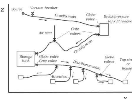
A gravity-driven water network (GDWN) is commonly used to deliver potable water from a source at a high elevation, such as a natural spring or reservoir, to households or pub-lic tap stands (Fig. 1). When feasible, gravity-driven water networks are attractive in comparison to pumped networks because of their simplicity and lower capital, operational, and maintenance costs. In addition, in many locations where GDWN are considered, there may be little or no access to reliable grid-based electrical power for pumps. To improve reliability, networks may be designed with loops or multiple water sources, although often material cost considerations re-strict attention to single-source branched networks.
Figure 1.Element schematic of a GDWN.
the node. Furthermore, application of the energy equation to each link in the network demonstrates that the design prob-lem is nonunique; i.e., choosing different pressure heads at the nodes will result in a different pipe diameter solution for the network, and thus different network costs. Minimiz-ing network cost will produce a unique solution to the de-sign problem, i.e., unique link diameters and nodal pressure heads.
In practice, gravity-driven water networks are commonly designed by a marching method, where diameters for each link of the network are chosen sequentially. After selecting a reasonable diameter for each link, the designer calculates the pressure head at the link outlet, and proceeds to the next link if this result is acceptable. In this way, the designer marches through the network until all pipe diameters have been se-lected. This method produces a feasible solution, but not a cost optimized one. As noted by Bhave (2003), cost savings of 20–30 % can result from the use of optimization tech-niques. In developing regions, the cost of a water network can be prohibitive, adding to the importance of optimizing network design.
Within the provided framework, the global optimum can be found through an exhaustive search of the solution space, known as complete enumeration, although this is infeasi-ble when considering networks with many links and diam-eter choices (Kadu et al., 2008; González-Cebollada et al., 2011). To reduce the computational time required by enu-meration, authors have proposed various partial enumeration methods which prune the search space (Kadu et al., 2008), although some of these techniques may remove the global optimum (Simpson et al., 1994). The most common types of algorithms that have been applied to optimize water network design include traditional deterministic methods, heuristic methods, metaheuristic methods, multi-objective methods, and decomposition methods (Zhao et al., 2016).
Deterministic methods include linear programming (LP), dynamic programming, and nonlinear programming (NLP),
and typically involve rigorous mathematical approaches (Zhao et al., 2016). A brief overview and comparison of these algorithms is given in Kansal et al. (1996), who use a single-part cost correlation for metric pipe diameters be-tween 100 and 350 mm. Linear programming techniques have relatively low computational complexity and allow each link to be composed of two diameters, called a split-pipe so-lution, although these may not always be practical to im-plement (Bhave, 1983; Kessler and Shamir, 1989; Swamee and Sharma, 2000; Samani and Mottaghi, 2006). LP can also get stuck in a local optimum (Zhao et al., 2016), although combining LP with metaheuristic techniques can help with the problem’s non-smoothness properties (Krapivka and Ost-feld, 2009). Dynamic programming has been used by Yang et al. (1975) and Martin (1980) to optimize networks in stages. This approach begins at the discharge nodes, proceeding to select feasible diameters and joints for upstream stages and storing these partial candidates in memory until the source node is reached. At this point, the algorithm reviews the fea-sible segment design options and selects a combination of stage solutions producing the lowest cost overall solution. This method, however, requires the designer to allow a rel-atively narrow range for the design pressure of each node, or otherwise store a large set of feasible candidate solutions in memory and also allow adjoining branches to arrive at differ-ent heads at the same node.
method of Jones also applies to serial and loop networks be-cause of its generality.
Heuristic methods follow specific rules to incrementally build better solutions, although the rules are not strictly for-mulated to trend towards local or global optima. An approach by Monbaliu et al. (1990) sets all network pipes to their min-imum size, where the pipe that has a maxmin-imum head loss gradient is incremented to its next-highest size until all nodal head requirements are satisfied. Similarly, an algorithm by Keedwell and Khu (2006) selects an initial solution and itera-tively responds to nodal head deficits and surpluses by incre-menting or decreincre-menting pipe sizes accordingly until a fea-sible solution is found. Suribabu (2012) proposed a heuristic that identifies pipes to increment or decrement in size based on flow velocity and alternative metrics such as proximity to the source node, achieving acceptable cost results with com-putational efficiency. While these algorithms are typically computationally efficient, they do not guarantee a global op-timum.
Metaheuristic optimization methods allow for a set of so-lutions to evolve through random processes that are guided with an objective function which rewards low network costs and penalizes hydraulic insufficiencies. Examples include evolutionary algorithms, which are most commonly genetic algorithms (Krapivka and Ostfeld, 2009; Simpson et al., 1994; Kadu et al., 2008; Prasad and Park, 2004), simulated annealing (Vasan and Simonovic, 2010; Tospornsampan et al., 2007), ant colony optimization (Maier et al., 2003), and differential evolution (Vasan and Simonovic, 2010). As re-viewed by Nicklow et al. (2010), evolutionary algorithms are an emerging popular alternative to the deterministic meth-ods, and they offer the opportunity to accommodate unique constraints and multiple design objectives. The main chal-lenges for evolutionary algorithms are the difficulty of incor-porating constraints into objective functions, the optimum se-lection of parameters, and a relatively large amount of com-putational effort. In addition to optimizing for cost, multi-objective methods, often based on evolutionary algorithms, allow the designer to choose from a Pareto optimal front of objectives, such as cost and reliability (Prasad and Park, 2004). In addition to water network design, metaheuristic al-gorithms have been used for a range of problems in water resources engineering, such as rainfall and runoff modeling (Taormina and Chau, 2015).
Decomposition methods involve the partitioning of net-works into smaller sub-netnet-works which are each optimized using one of many types of techniques and then combined into an overall solution. In some cases, the loops in the sub-networks are removed, producing branching trees which are then optimized individually. Techniques used to optimize the sub-networks can involve multiple methods, including lin-ear programming (Saldarriaga et al., 2013) and differential evolution (Zheng et al., 2013), with a later stage optimizing the network as a whole using the sub-network solutions as inputs. Note that another distinct use of the term
“decompo-sition” refers to the approach of iteratively solving “inner” and “outer” mathematical problem formulations, and has been used in the literature by Krapivka and Ostfeld (2009) who traces its use in this context back to Alperovits and Shamir (1977).
In the present study, we present three algorithms, each from one of three major categories of methods applied to the cost optimization of water distribution networks, and compare their performance on five cases adapted from real GDWNs. These algorithms include (1) the calculus-based (CB) optimization model of Jones (2011), an NLP method; (2) backtracking (BT), a partial enumeration method; and (3) a genetic algorithm (GA), a metaheuristic method. Ma-jor distinguishing features of these algorithms include their working use of continuous diameters (CB) versus discrete diameters (BT and GA), their deterministic (CB and BT) ver-sus stochastic (GA) search process, and their relative scala-bility as better (CB, GA) and worse (BT) for larger networks. In terms of their ability to find a global optimum solution for the problem formulation, CB finds a global optimum for con-tinuous diameters but cannot guarantee a discrete diameter global optimum in its mapped solution, BT can guarantee a discrete global optimum, and GA cannot guarantee an opti-mum. For a direct comparison of techniques, the pipe costs used for all algorithms are found by interpolating a two-part cost formula based on a curve fit of real cost data for avail-able diameter values. The three algorithms are tested against networks adapted from field data on five actual GDWNs in-stalled in Panama, Nicaragua, and the Philippines.
Within the broader context of water network problem for-mulations, this paper is concerned with finding cost-optimal single-diameter solutions to branching water distribution net-works with steady-state demand flows and pre-specified pipe locations. By implication of being gravity-driven, the lem does not involve the use of pumping stations. This prob-lem formulation is directly applicable to typical gravity-driven water networks, and is also useful for multi-objective algorithms, the consideration of sub-networks in a decompo-sition technique, pumped networks, and looped system opti-mization, which can involve reformulating the problem into a branching configuration.
inter-est in this work, and for smooth and commercial steel rough-ness values.
2 Problem formulation
Branching networks are considered (Fig. 1), where all branches connect a distribution main node with a delivery node, shown as tap stands or houses. For each link in a network ofNL links, pipe length (L) and the net elevation
change (1z) are considered known and fixed. Steady-state flow rates (Q) are prescribed for each link based on the de-mand flow data at delivery nodes. As noted above, dede-mand flows are determined by community surveys and extrapolated in time to quantitatively account for population growth. Mi-nor losses are accounted for through a miMi-nor loss coefficient K or a dimensionless equivalent pipe length, (Le/D, or in
symbol form,LebyD), whereLeis the pipe length of
diame-terDwhose frictional loss results in the corresponding mi-nor loss. An optimal solution is obtained by selecting pipe diameters (D) from a set of commercially available diame-ters such that the network’s material cost is minimized. With NDchoices of diameters forNLlinks, the problem hasNDNL
candidate solutions.
For all nodes, pressure head, h, is greater than or equal to a chosen minimum, hmin. The value forhmin is selected
to eliminate possible leakage of contaminated ground water into the network should the operating conditions change in an unanticipated way. The change in pressure head,1h, across each link is calculated with the energy equation for pipe flow as follows:
1h= −1z+
α+K+f
L
D+LebyD
8Q2
π2gD4, (1)
where for each link,αis the kinetic energy correction fac-tor and f is the Darcy friction factor, calculated with the Colebrook–White equation (Colebrook and White, 1937) or Churchill correlation (Churchill, 1977), andgis acceleration of gravity. The kinetic energy correction factor,α, is consid-ered only in the first link, where acceleration from a zero-velocity source is sometimes non-negligible for the smallest of GDWNs that have been encountered. Thus,
α=
2 Re≤2300 1.05 Re>2300,
whereReis the Reynolds number for pipe flow, 4Q/π νD, andνis the kinematic viscosity of water. The possibility of laminar flow (Re≤2300) is permitted since branches from the smallest GDWN observed in practice have been in this regime.
The pressure upper bound is not incorporated into the op-timization process. Worst-case pressure conditions occur un-der hydrostatic conditions, which are directly related to the maximum elevation change in the network and where no flow occurs. Therefore, before the optimization process is under-taken, the selections of appropriate pressure ratings for the
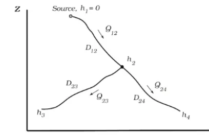
Figure 2.Three-pipe branch network.
pipe and, if needed, break-pressure tanks are left to the cor-rect judgment of the designer under no-flow conditions. In addition, precautions against water hammer are left to the designer.
3 New calculus-based algorithm
In this section we develop a new calculus-based algorithm for pipe diameters that minimize overall pipe cost for the network. First appearing in Jones (2011), this algorithm is solved simultaneously with the energy equation for each link to produce unique solutions forD and nodal pressure head values that minimize network pipe cost, as opposed to only the distribution main cost as in Swamee and Sharma (2000). The method also applies to serial and loop networks but the focus for the present work is on branching networks.
We assume continuous pipe diameters in this section; val-ues that result from the solution of the energy equation. Map-ping between continuous diameters and the discrete nominal sizes, required to complete the design, will be addressed be-low.
Consider the three-pipe network shown in Fig. 2. Pipes 1– 2, 2–3, and 2–4 meet where headh2is unknown. Each pipe
has a prescribed volume flow rate and length and unknown diameterDas shown. The change in elevation between the top and bottom of each pipe is1z, and1his the change in pressure head. There is a prescribed head at each outlet for pipes 2–3 and 2–4.
The Blasius equation has higher accuracy (2 % for low Re
and 3 % for highRe) in the range 104<Re< 105, over which most of the GDWNs in this work operate, compared with the Swamee–Jain correlation of +8 %/−3 %, thus the Bla-sius equation is chosen for this work. A combination of the Blasius equation with the energy equation gives explicit for-mulas forDfor the three links in Fig. 2. For simplicity, and to reduce the number of free parameters, the conditions for pipes 2–3 and 2–4 are assumed to be identical without loss of generality. We therefore obtain
D12=0.741
1z12+1h12 L1
−4/19
Q12ν1/7 g4/7
7/19
(2)
D23=D24=0.741
1z23+1h23 L2
−4/19
Q23ν1/7 g4/7
7/19
.
With our assumptions and inspection of Fig. 2,1h12= −h2
and1h23=1h24=h2−h3=h2−h4, we furthermore
ob-tain
D12=0.741
1z12−h2 L1
−4/19
Q12ν1/7 g4/7
7/19
(3)
D23=D24=0.741
1z23−h3+h2 L2
−4/19
Q23ν1/7 g4/7
7/19
.
The single-part pipe-cost model can be assumed to follow a power-law relationship (Swamee and Sharma, 2008)
C=a
D Du
b
, (4)
whereC is cost per unit length of pipe,a is a constant co-efficient, bis a constant exponent, andDu an assumed unit
diameter. A more robust, two-part model, valid for a greater range of pipe sizes than that of Swamee and Sharma (2008), will be used below. The use of pipe material cost as the ob-jective function was assumed because of relevance. In most GDWNs of interest in this work, installation labor comes from the local community and has no well-defined associ-ated cost, such that the material cost for the network is of prime importance. For a more general case, the economics of a GDWN may be more encompassing and include mate-rials, labor, operation and maintenance, depreciation, taxes, and salvage, among others. The time value of money may also need to be considered, which includes interest rates and estimation of the network lifetime.
With Eq. (4) the general expression for the total cost for the pipe material,CT, is obtained by summing over all links ij,
CT=a
X
ij Lij
D
ij Du
b
, (5)
which, for the present problem, becomes
CT=a
"
L12
D
12 Du
b
+L23
D
23 Du
b
+L24
D
24 Du
b#
=a
"
L12
D
12 Du
b
+2L23
D
23 Du
b#
. (6)
The mathematical basis for a unique solution forh2with
cost minimization is now presented. In addition to the fixed pipe lengths, the total cost depends on the diameters for all pipes in the network. For the case of Fig. 2, where we now allow pipe 2–3 and pipe 2–4 to be different, we get
CT=CT(D12(h2), D23(h2), D24(h2)). (7)
Using the chain rule from the calculus, the total differential of Eq. (7) is
dCT= ∂CT ∂D12
∂D12 ∂h2
dh2+ ∂CT ∂D23
∂D23 ∂h2
dh2
+ ∂CT ∂D24
∂D24 ∂h2
dh2. (8)
The minimum value ofCTis found once dCT=0 (and once
it is verified that the second derivative ofCTis positive thus
indicating thatCTis indeed a minimum). Requiring this, we
obtain
0= ∂CT ∂D12
∂D12 ∂h2
+ ∂CT ∂D23
∂D23 ∂h2
+ ∂CT ∂D24
∂D24 ∂h2
. (9)
The cost CT is from Eq. (5), so the derivatives like ∂CT/∂D12in Eq. (9) are written in general as
∂CT ∂Dij
=ab Dijb−1
Db
u
Lij (10)
for any linkij.
The derivatives like∂D12/∂h2in Eq. (9) are obtained by
taking the partial derivative of the pipe diameter with respect to the relevant pressure head in the appropriate energy equa-tion. For the full energy equation, whereDappears in a non-linear way in more than one location, this would be done using numerical methods. However, if we assume minor-lossless, smooth-turbulent flow as noted above, we can use the energy equations like Eq. (3). We therefore obtain the following for pipe 1–2:
∂D12
∂h2
=0.156
1z
12−h2
L12
−1923 ν1/7Q
12
g4/7L19/7 12
!197
; (11)
for pipe 2–3, we get
∂D23 ∂h2
=
−0.156
1z23+h2−h3 L23
−1923
ν1/7Q23
g4/7L19/7 23
!197
; (12)
and for pipe 2–4,
∂D24 ∂h2
= −0.156
1z
24+h2−h4 L24
2319
ν17Q24
g47L 19
7
24
7 19
Equations (10)–(13) are combined with Eq. (9) to produce a single algebraic equation that depends onh2, as well asD12, D23, andD24. IntroducingD12, D23, andD24 from Eq. (3)
into this algebraic equation, we get
0=Q712b/19
1z
12−h2
L12
−(1+4b/19)
−Q723b/19
1z23+h2−h3 L23
−(1+4b/19)
−Q724b/19
1z
24+h2−h4
L24
−(1+4b/19)
. (14)
The general form of Eq. (14), written at any internal node is
0=X ij,in
Q7ijb/19Sij−(1+4b/19)−X ij,out
Q7ijb/19Sij−(1+4b/19), (15)
where the hydraulic gradient,Sij, is
Sij =
1zij+1hij Lij
. (16)
In Eq. (15) the indicesij,in andij,out on the summations refer to inflows and outflows at the node (e.g., in Fig. 2, ij,in=12 andij,out=23 and 24). Equation (15), the new CB algorithm proposed in this work, is written for each in-ternal node in the network and solved simultaneously with the energy equation for each link to obtain unique and opti-mal values ofDijfor all links andhjfor all internal nodes. It is understood that the nodal pressure heads determined from the solution of this system must be greater than or equal to the hmin prescribed for the network. For nodes that do not
satisfy this condition, the pressure head is set equal tohmin,
as part of the CB algorithm. Thus,hj≥hmin.
Minor losses using the equivalent-length method can be included in the above developments by artificially extending the length of the link byLein which minor loss occurs, thus
contributing a non-zeroLebyDterm in Eq. (1). We also extend
the cost model of Eq. (5) from Swamee and Sharma (2008) to encompass two different ranges of pipe diameters having two different coefficients a and exponents b. The link between the two ranges starts at discrete pipe sizeDco, at and below
which the cost model for the small (subscript s) pipe sizes applies, and discrete pipe size Dco+1, at and above which
the cost model for the large (subscript l) pipe sizes applies. The cutoff diameter,Dcois chosen by the designer based on
inspection of cost vs. diameter data. Thus,
Cij=Lij
as D ij Du bs ,
Dij≤Dco
c1+c2 Dij
Du +c3
D
ij Du
2
+c4
D
ij Du
3
,
Dco< Dij< Dco+1
al D ij Du bl ,
Dij≥Dco+1.
(17)
In Eq. (17),asandalare the coefficients for the small
(desig-nated by subscripts) and large (subscriptl) pipe size regions, respectively, and bs andbl are the exponents for the small
and large pipe size regions, respectively. A cubic spline is fit between pipe sizesDcoandDco+1to complete the transition
between small and large pipe sizes. The coefficients of this polynomial arec1,c2,c3, andc4as seen in Eq. (17). These
coefficients are evaluated by matching the cubic polynomial and pipe data atDco andDco+1 and the first derivative of
the polynomial with respect to Dij/Du to asbs
Dco Du
bs−1
at Dij=Dco and to albl
Dco
+1 Du
bl−1
at Dij =Dco+1. An
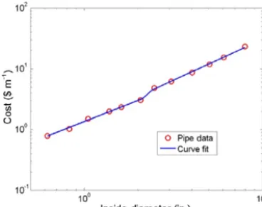
example of data for polyvinyl chloride (PVC) pipe and the curve fit is shown in Fig. 3. The results of the curve fit are as follows: Dco=2.067 in., Dco+1=2.469 in., as=USD 1.349 m−1, bs=1.157, al=USD 1.381 m−1, bl=1.344,c1=USD 237.516 m−1,c2=USD 316.125 m−1, c3=USD 140.450 m−1,c4= −USD 20.499 m−1. It is clear
from inspection of Fig. 3 that a one-part cost model would not have produced an acceptable curve-fit to pipe-cost data.
With the inclusion of the two-part cost model and minor loss term, Eq. (15) becomes
0=
P
ij,in
Cij0 A 4 19
ij 1+ij
194 S− 23 19 ij
Q7ijν g4D19u
1
19
1−BA 4 19
ij
0
ij 1+ij
−1519
S− 4 19 ij Q7 ijν
g4D19 u
191
−P
ij,out Cij0A
4 19
ij 1+ij
194 S− 23 19 ij
Q7ijν g4D19
u
1/19
1−BA 4 19
ij
0
ij 1+ij
−1519
S− 4 19 ij Q7 ijν
g4D19 u
1/19,
(18)
whereB=0.1989 and
ij= X k L e D k,ij Dij Lij (19)
ij0 =X k L e D k,ij Du Lij
Aij=
0.318, smooth pipe
0.420, steel pipe (20)
andAaccounts for the effect of pipe roughness (smooth and commercial steel). The termCij0 is the derivative of the cost function per unit length with respect toD/Du. For the
two-part cost model from above, we obtain
Cij0 =
asbs
D
ij Du
bs−1
,
Dij ≤Dco
c2+2c3
D
ij Du
+3c4
D
ij Du
2
,
Dco< Dij< Dco+1
albl
D
ij Du
bl−1
,
Dij ≥Dco+1.
Figure 3.PVC pipe cost from 2011 data.
Equation (18), and its simpler form Eq. (15) for minor-lossless flow and a single-part pipe-cost model (it is easy to show that Eq. (18) regresses to Eq. (15) for these con-ditions), is the root of the calculus-based optimization in this work and is applied at all internal nodes to uniquely determine hj. Equation (18) is valid over the range of ∼4000 <Re<∼300 000. Algorithms to solve a general set of independent, nonlinear algebraic equations using, for ex-ample, the Levenberg–Marquardt, quasi-Newton, Newton– Raphson, or conjugate gradient methods are available in most commercial math packages including Matlab (1 Apple Hill Drive, Natick, MA USA 01760) and Mathcad (http://www. ptc.com 31 January 2018). We used the package Mathcad in the present work. Thus, compared with an iterative solution procedure, a solution flowchart is not relevant here.
Bhave (1978) first proposed an algorithm like Eq. (15) us-ing slightly different notation than here. For clarity, we re-present Eq. (15) using Bhave’s notation as
0=XQ7ijb/19Sij−(1+4b/19)−XQ7j kb/19Sj k−(1+4b/19),
where the ij andj k notation are shown in Fig. 4. Indexj spans all internal nodes along the distribution main. A quanti-tative comparison between Eq. (18) and the method of Bhave is presented below.
4 Backtracking algorithm and genetic algorithm
Backtracking (BT) and genetic algorithm (GA) assess candi-date solutions composed of discrete diameters from a com-mercially available set. These candidates are represented by a vector ofNLelements where each element corresponds to a
commercially available diameter of a network link. To reduce the computational time associated with these evaluations, the constraints imposed by the energy equation and cost mini-mization may be more efficiently evaluated through lookup tables. With fixed L, 1z, K, LebyD, and α, the change in
pressure head1his evaluated for allND×NLcombinations
Figure 4.Bhave (1978) index notation at an internal node,j.
of pipe diameter and link index:
1h=
1h11 · · · 1h1NL ..
. . .. ... 1hND1 · · · 1hNDNL
. (22)
While an algorithm evaluates a candidate solution, the pres-sure head at each node is sequentially calculated by “march-ing” through the network. Starting with the fixed source pres-sure head, the algorithm finds the prespres-sure headhifor a given node by adding the head at the upstream node,hi−1to the
change in head for that link iL and the diameter iD under
consideration. Thus,
hi=hi−1+1h(iD, iL). (23)
Along with the hydraulic evaluation of a candidate solution, the cost of the partial candidate is found through the use of a lookup tableC:
C=
C11 · · · C1NL ..
. . .. ... CND1 · · · CNDNL
, (24)
whereC(iDiL) returns the additional cost of assigning a
di-ameter with indexiDto linkiL. In this way, the candidate
so-lution’s hydraulic performance and cost are incorporated into the genetic algorithm and backtracking approaches. In con-trast to GA, the backtracking algorithm evaluates pressure head and cost upon consideration of each partial candidate, where GA calculates these values on full candidates as part of the objective function.
4.1 BT and GA pre-processor 1: maximum available diameter
their cost exceeds that of an already-found viable candidate. Therefore, a pre-processor is used to provide a maximum di-ameter (Dmax) that should be considered during the
optimiza-tion process. This procedure, which produces a conservative estimate, finds the smallest diameter at which a network with a single pipe diameter choice produces no nodes with a pres-sure head belowhmin, similar to the technique used by
Mo-han and Jinesh Babu (2009). After this diameter is found, the next larger diameter in the set is selected asDmaxto
al-low the algorithm to select a larger than necessary diame-ter if this is able to save cost elsewhere. It worth noting that Kadu et al. (2008) presents another method to further prune the search space with the critical path concept, where Don-gre and Gupta (2011) noted the computational advantages of having just four diameter choices per link. This method, how-ever, may prune the global optimum and may not produce feasible head values at intermediate nodes, as in the case of networks with a local high point.
4.2 BT and GA pre-processor 2: adjusted minimum pressure head
A second pre-processor adjusts the minimum pressure head requirement for each internal node by considering the total head required at downstream nodes. It can be recognized that, without the use of a pump, the total head cannot increase at nodes downstream of a given nodei. Furthermore, the total head must decline at a minimum grade that is determined by the demand volume flow rate and the largest pipe diameter available (Dmax) for selection. This energy constraint is
uti-lized to reduce the number of candidates to be considered by increasing the minimum pressure head at nodes where these rules produce a higher minimum head than the orig-inal hmin. For example, nodes upstream of a local network
high point can have their minimum pressure head increased beyond the normal minimum, since the pressure head must be great enough to ensure adequate flow to the higher eleva-tion downstream node. To begin this process, each nodeiis initialized with a baseline minimum total head:
t hmin,i=zi+hmin. (25)
t hmin,i is thus initialized by considering only the node’s hy-draulic requirements in isolation, i.e., without acknowledg-ing the neighboracknowledg-ing downstream nodes. The pre-processor then considers updating t hmin,i by checking the following condition, which is false when the minimum pressure head at downstream nodes produces further constraints on an up-stream nodei. Thus, for all nodesi which are upstream of some nodej, the following inequality can be evaluated:
t hmin,i−t hmin,j≥ (26)
αi−j+Ki−j+fi−j
L
i−j Di−j
+LebyDi−j
8Q2
i−j π2gD4
max .
Also, consider that when flow rateQi−j is small andDmax
is large, the right-hand side of Eq. (26) approaches zero, rep-resenting the simple statement that upstream total head must always be greater than downstream total head. When the con-dition in Eq. (26) is false, the minimum total head can be up-dated in nodeisuch that the maximum diameter size in link i−j is able to meet the downstream node’s minimum total head, or
t hmin,i=t hmin,j+ (27)
αi−j+Ki−j+fi−j
L
i−j Di−j
+LebyDi−j
8Q2
i−j π2gD4
max .
In this way,t hmin,i may be updated for each node until the condition in Eq. (26) is true for all nodesiwith a downstream nodej connected by a single link.
After the values fort hmin,iare updated, they are converted back into minimum pressure head values by subtracting the elevationzi fromt hmin,i. This pre-processor serves to nar-row the search for viable candidate solutions by potentially increasing the minimum pressure head. Since backtracking and GA consider network links in the downstream direc-tion, these algorithms are otherwise blind to future down-stream pressure head requirements. This limitation is alle-viated by the pre-processor, which allows these algorithms some implicit information about what local diameter choices will be viable for the full network solution. Note that both pre-processors discussed will not prune the global optimum from the solution.
4.3 Backtracking algorithm (BT)
The backtracking algorithm is a partial enumeration method that employs a systematic search of candidate solutions to find a global optimum. The algorithm works recursively to incrementally build candidate solutions while checking the candidates for hydraulic and cost acceptability. The strength of the BT is that, upon discovery of an infeasible partial candidate, all extensions of that candidate can be elimi-nated from consideration. In this way, many solutions can be pruned from the solution tree to achieve greater computa-tional efficiency.
contin-ues searching once it has found its first feasible solution and uses pre-processors 1 and 2 to further reduce the search space. This implementation of BT, however, scales poorly with larger network sizes and would not be appropriate for use on large urban networks. Its appropriateness is shown here for many of the GDWNs encountered in practice, as ev-idenced by its use on real-world GDWN test cases in this pa-per. Moreover, it serves as a benchmark against which other algorithms can be compared.
BT uses two rejection criteria to discard candidate solu-tions from further consideration. The first rejection crite-rion is that when a candidate violates pressure head con-straints, all candidates with equal or lesser diameter sizes can be discarded. This condition is leveraged even more effec-tively with pre-processor 2 above, which can increase pres-sure heads at individual nodes by anticipating the head re-quirements at surrounding nodes. The second rejection crite-rion is that once a feasible candidate has been found, all other partial candidates with a higher cost can also be discarded. The BT algorithm further extends this second criterion by considering that the links yet to be considered in a partial candidate, an “extension” to the partial candidate, will cost at a minimum that of the entire extension being composed of the smallest available diameter.
The backtracking algorithm begins its search of the solu-tion tree by considering the partial candidate with the small-est diameter size assigned to the first network link. The pres-sure head and the partial candidate cost at the outlet node are calculated with the1handClookup tables. If this par-tial candidate meets pressure head and cost requirements, the algorithm extends this partial candidate by assigning the smallest diameter to the downstream link. If a partial can-didate produces a node that is rejected on the basis of pres-sure head, the next largest larger diameter is chosen for the link upstream of the node. If no diameter satisfies the pres-sure head condition, the algorithm backtracks to the upstream link and assigns a larger diameter to the link. In this way, the algorithm continues to extend and reject candidate solutions until a full candidate satisfies the pressure head requirements. Once a working solution has been found, candidate solutions may be rejected based on cost. For each new candidate, cost is calculated by adding the cost of diameters that have al-ready been assigned to the cost of assigning all downstream links with the smallest diameter available. If this cost exceeds the cost of the running optimum, the partial candidate is re-jected. While the minimum pressure head criterion tends to prune candidates with diameters that are too small, the cost-based criterion tends to prune candidates of diameters that are too large.
4.4 Modified backtracking algorithm (BT-NoUp)
A modification to the BT algorithm was made to further im-prove its computational speed, although at the risk of pruning the global optimum from the search. This modified algorithm
(BT-NoUp) rejects all candidates that feature a smaller di-ameter that is upstream of a larger didi-ameter when an equal or smaller flow rate is present in the downstream link. Typi-cally, a network designer would not consider such designs, and in cases where a single source feeds into a network with constant-length links, it is advantageous (or equiva-lent) to place larger diameters upstream of smaller diameters. However, due to the discrete nature of diameter choices and link lengths, an optimization problem may, in fact, have an optimal candidate with a larger diameter downstream from smaller ones. For this reason, the BT-NoUp algorithm, un-like the BT algorithm, may miss the global optimum at the expense of its greater computational efficiency.
4.5 Genetic algorithm (GA)
Genetic algorithms are stochastic optimization techniques that mimic the process of natural selection, and numer-ous variations of GAs have demonstrated acceptable perfor-mance on WDN design (Nicklow et al., 2010). Given their popularity, the GA included in this study is meant to provide a point of comparison to the BT and CB algorithms when applied to GDWNs.
When implemented in water network design, each candi-date solution represents a selection of pipe diameters. The algorithm is initialized with a population of candidates of sizeNcthat repeatedly undergoes the processes of mutation,
crossover, and selection
ci = D1,i D2,i . . . DNL,i, (28)
where each candidate in the populationci containsNL
di-ameters. In the present work, candidates are represented as a string of natural numbers, which is used over a binary repre-sentation to improve the ease of encoding (Vairavamoorthy and Ali, 2000). The mutation operator replaces pipe diam-eters with a diameter from a uniform random distribution, where each link diameter has a probability ofpmut of
mu-tating on each generation. The crossover operator randomly pairs individuals in the population with probability pxover
and performs a single-point crossover of the two individu-als, where the point of crossover is randomly chosen. The fitness,fi, of each candidate is assessed with penalties as-sociated with the solution’s pipe cost,Cpipe,i, and hydraulic
cost,Chyd,i, which is assigned when violations of the
pres-sure head requirements occur:
fi=
1 Cpipe,i+Chyd,i
. (29)
The hydraulic cost is found for each individual by identify-ing nodes in which the pressure head is less thanhmin and
multiplying the total amount of head violation by a hydraulic penalty coefficient,ahyd:
Chyd,iC =ahyd NL
X
1
hmin−hiN
To allow for a hydraulic penalty coefficient to produce similar results in both small-scale (inexpensive) network and a large-scale (more expensive) cases, the hydraulic penalty coefficient is made directly proportional to the average so-lution cost. With each generation,ahydis updated by
multi-plying the normalized penalty coefficient,ahyd,norm, by the
average pipe cost of the population,
ahyd=ahyd,norm
Nc
P
1 Cpipe,iC
Nc
. (31)
The algorithm then selects candidates to be carried into the next generation with a tournament selection method, where Nc groups of s individuals are randomly assigned and the
fittest candidate among each group is selected, thus replacing the previous population with an equally sized population of Ncindividuals.
In this study, the genetic algorithm parameters used were Nc=200,pmut=0.05,pxover=1,Ngen=500,ahyd,norm=
0.05, ands=10. These parameters were chosen by system-atically varying parameter values until the optimum cost of a network, case 2, could no longer be significantly improved. The first four of these values are in line with typically used values from Simpson et al. (1994) of Nc (30–200), pmut
(0.01–0.05),pxover(0.7–1.0), andNgen(100–1000).
5 Cases studied
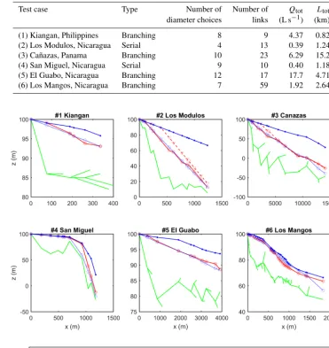
Six cases were studied based on actual GDWN in Panama, Nicaragua, and the Philippines. Global characteristics of each network are presented in Table 1 and the details of each network are presented in Table 4a–f. Each network is a branching type without loops. The total lengths of the works range from less than 1 to over 15 km. Two serial net-works are tested to demonstrate the effect of a local high point on the algorithm solutions. Elevation plots for each case are shown in Fig. 5.
The choice ofhminis not standardized, and should
appro-priately balance the risk of negative pressure in pipes and the increase in network cost due to the requirement of using larger diameters. The choice ofhminin GDWN design is
typi-cally in the range of 5–20 m (Arnalich, 2010; Bouman, 2014; Swamee and Sharma, 2008). In the present studyhmin=7 m,
although this requirement was reduced at selected nodes at the beginning of a network where changes in elevation are still small (case 2, where the pressure head at node 2 is re-laxed to 2 m). At the source node, the pressure head is fixed at atmospheric pressure. All cases assumed minor-lossless flow, although all algorithms (e.g., Eq. 18 for CB-Theor) are capa-ble of handling minor loss coefficients through the equivalent length method as described above. All algorithms were run in a late-version of MATLAB (or Mathcad for CB) on an Intel i5 processor at 2.50 GHz.
6 Mapping the theoreticalDto discrete pipe sizes
The mapping between continuous diameters and the discrete nominal pipe sizes was accomplished in our solution in one of the following ways:
1. For small and moderate size networks, the designer may manually adjust the pipe sizes (downward, normally one pipe size) starting from the first link downstream from the source and continuing along the rest of the distribu-tion main to the end in a step-by-step manner. A nearby plot of the pressure heads compared with the theoretical Dij from the CB approach (e.g., on the same Mathcad page for our solution) will highlight the acceptability or unacceptability of any change. This exercise also gives the designer valuable understanding of the sensitivity of the design to small changes in pipe sizes.
2. Based on the theoretical Dij from the CB approach, a split-pipe can be created for each link. That is, the lengths for the two discrete pipes sizes that bound the theoretical Dij from above and below are calculated such that the pressure drop between two consecutive nodes in the distribution main matches between the composite pipeline and the CB approach. This also pro-vides discrete pipe sizes that nearly match the CB solu-tion in terms of cost.
7 Results
The current study evaluated three types of algorithms that op-timize the design of gravity-driven water networks (GDWN). The algorithms include the calculus-based (CB) algorithm (Eq. 18), a backtracking algorithm (BT) and its modified ver-sion (BT-NoUp), and a genetic algorithm (GA). The algo-rithms were applied to six test cases that are based on real GDWNs. Our results show that the CB, GA, and BT-NoUp algorithms could find solutions to the GDWNs within 25 % of the BT global optimum. All cases assume minor-lossless flow and a two-part pipe-cost model. Solution costs from each algorithm are shown in Table 2 and runtime statistics are shown in Table 3. BT could run to completion in < 1 min in all but the largest case (case 6 with 59 links), which did not complete after 7 days. As such, cost comparisons to BT are not made for case 6.
map-Table 1.Characteristics of test cases.
Test case Type Number of Number of Qtot Ltot
diameter choices links (L s−1) (km)
(1) Kiangan, Philippines Branching 8 9 4.37 0.82
(2) Los Modulos, Nicaragua Serial 4 13 0.39 1.24
(3) Cañazas, Panama Branching 10 23 6.29 15.2
(4) San Miguel, Nicaragua Serial 9 10 0.40 1.18
(5) El Guabo, Nicaragua Branching 12 17 17.7 4.71
(6) Los Mangos, Nicaragua Branching 7 59 1.92 2.64
Figure 5.Network elevation (z) and hydraulic grade lines (HGLs) of algorithm solution for main distribution links.
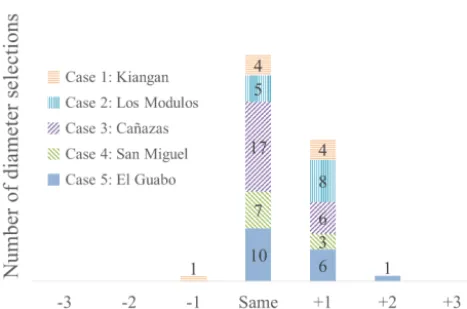
ping process used in this study simply mapped each theoreti-cal diameter to the nearest available diameter of a larger size, thus producing a solution which still satisfies static head re-quirements but with a higher associated material cost. This tended to oversize the diameters, although the CB-Disc solu-tions were always within two diameters of the known global optimum solutions, as shown in Fig. 6. From all the com-bined test cases with known global optima, all but one (71 out of 72) of the diameter selections were within one di-ameter of the global optimum. More sophisticated mapping schemes, like independently adjustingDfor each link in the distribution main in a step-by-step manner starting with the source while ensuring all pressure head constraints are satis-fied, would be more likely to produce results identical to the global optimum (see Sect. 6). This was performed in the cur-rent study but the results are not presented because of space
constraints. The CB-Disc solution costs were, in all cases, larger than the global optimum, with costs ranging from 3.9 to 22.6 % above the global optimum. Thus, for all cases, the calculus-based algorithm bounded the cost of the global op-tima with a lower-cost CB-Theor solution and a higher-cost CB-Disc solution. This trend is a result of the additional con-straints imposed by the finite set of diameter choices. If the algorithm is allowed a greater number of discrete diameter choices, i.e., through adding a less-common nominal diame-ter size to the available set, the cost of the CB-Disc solution would approach the CB-Theor solution. For all but case 6, the CB algorithm converged on a solution in 3 min or less.
opti-Table 2.Solution costs for each algorithm.
Case Solution cost (USD) Percentage cost increase over Percentage cost increase
BT (global optimum) over CB-Theor
BT BT-NoUp CB-Theor CB-Disc GA BT-NoUp CB-Theor CB-Disc GA BT BT-NoUp CB-Disc GA
(1) Kiangan, Philippines 2331 2331 2257 2594 2337 0 −3.2 11.3 0.3 3.3 3.3 14.9 3.5
(2) Los Modulos, Nicaragua 1441 1472 1404 1767 1445 2.1 −2.6 22.6 0.3 2.7 4.8 25.9 2.9
(3) Cañazas, Panama 72 190 72 443 68 245 84 441 73 964 0.4 −5.5 17.0 2.5 5.8 6.2 23.7 8.4
(4) San Miguel, Nicaragua 5418 5418 5172 5627 5422 0 −4.5 3.9 0.1 4.8 4.8 8.8 4.8
(5) El Guabo, Nicaragua 61 445 61 445 59 506 73 886 63 113 0 −3.2 20.2 2.7 3.3 3.3 24.2 6.1
(6) Los Mangos, Nicaragua ∗ 4082 3670 4405 4339 ∗ ∗ ∗ ∗ ∗ 11.2 20.0 18.2
∗Note: BT did not complete after 7 days of runtime.
Table 3.Runtime and size of solution space for each algorithm.
Case Runtime Number Number of Possible candidate Partial candidates
of links diameter choices solutions considered
BTa BT-NoUpa CB GAa BT BT-NoUp
(1) Kiangan, Philippines 0.2 s 0.05 s < 3 min 1 s 9 8 1.3×10⁸ 269 126
(2) Los Modulos, Nicaragua 7 s 0.04 s < 3 min 2 s 13 4 6.7×10⁷ 48 886 210
(3) Cañazas, Panama 40 s 0.1 s < 3 min 2 s 23 10 1.0×10²³ 433 210 2367
(4) San Miguel, Nicaragua 0.5 s 0.04 s < 3 min 2 s 10 9 3.5×10⁹ 3671 244
(5) El Guabo, Nicaragua 0.5 s 0.05 s < 3 min 2 s 17 12 2.2×10¹⁸ 3810 423
(6) Los Mangos, Nicaragua > 7 dayb 2 s 94 min 5 s 59 7 7.3×1049 b 44 374
aBT, BT-NoUp, and GA algorithm run times do not include approximately 2 s of pre-processing time.bBT did not complete case 6 after 7 days of runtime.
Figure 6.Diameter sizes from calculus-based (CB-Disc) solutions compared with global optimum solutions (from backtracking, BT). A global optimum for case 6, Los Mangos, is not included since BT did not complete after 7 days of runtime.
mum. BT-NoUp missed the global optimum in cases 2 and 3, although by a small percentage increase in cost (2.1 and 0.4 % respectively). BT-NoUp, however, finished its search in a shorter amount of time in comparison to BT, a bene-fit that becomes relevant on problems with larger solution spaces, such as cases 3 (1.0×10²³candidate solutions) and case 6 (7.3×1049candidate solutions).
GA was run on each case a total of 100 times, each run it-self evolved 200 candidates for 500 generations. The lowest-cost candidate amongst the final population that did not vi-olate the pressure head condition was chosen as the GA so-lution. Because GA is a stochastic search algorithm produc-ing different results from run-to-run, the costs of the optima from all 100 runs were averaged, with this averaged value presented in Table 2. Overall, GA costs came close to the global optima (within 3 %) for cases 1–5 where the global optimum was known from BT. GA solution costs increased with larger network sizes, with its solution cost 18 % higher than CB-Theor for case 6, the largest case run. Each GA run finished consistently within 1–5 s, not including about 2 sec-onds of pre-processor time. We note that variations of GAs have been reported in the literature and several of these may improve upon the GA results obtained in this study. Poten-tial improvements to the GA a self-adapting penalty func-tion (Wu and Walski, 2005), the use of elitism to preserve the best solutions (Kadu et al., 2008), and a reduction in the search space (Kadu et al., 2008). One reported improvement, the scaling of the fitness function to magnify the rewards to-wards slightly fitter candidates at later generations (Dandy et al., 1996), was attempted for case 2 but did not result in a noticeable effect on performance.
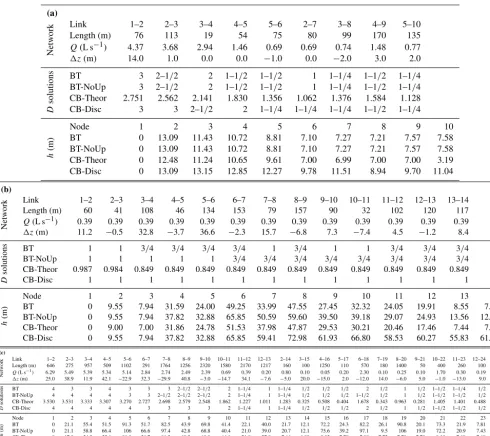
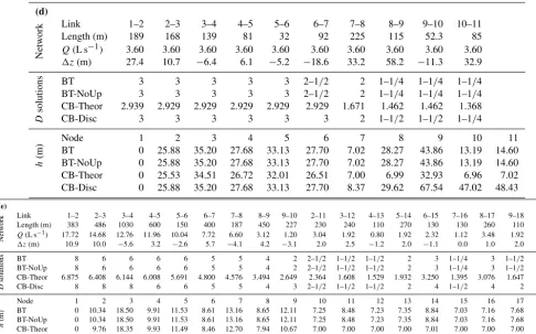
Table 4.Case network properties, diameter (D) results (inch nominal sizes, with CB-Theor in inches), and nodalh(in meters) for (a) Case 1, Kiangan, (b) Case 2, Los Modulos, (c) Case 3, Cañazas, (d) Case 4, San Miguel, (e) Case 5, El Guabo, and (f) Los Mangos.
(a)
Netw
ork
Link 1–2 2–3 3–4 4–5 5–6 2–7 3–8 4–9 5–10
Length (m) 76 113 19 54 75 80 99 170 135
Q(L s−1) 4.37 3.68 2.94 1.46 0.69 0.69 0.74 1.48 0.77 1z(m) 14.0 1.0 0.0 0.0 −1.0 0.0 −2.0 3.0 2.0
D
solutions
BT 3 2–1/2 2 1–1/2 1–1/2 1 1–1/4 1–1/2 1–1/4
BT-NoUp 3 2–1/2 2 1–1/2 1–1/2 1 1–1/4 1–1/2 1–1/4
CB-Theor 2.751 2.562 2.141 1.830 1.356 1.062 1.376 1.584 1.128
CB-Disc 3 3 2–1/2 2 1–1/4 1–1/4 1–1/4 1–1/2 1–1/4
h
(m)
Node 1 2 3 4 5 6 7 8 9 10
BT 0 13.09 11.43 10.72 8.81 7.10 7.27 7.21 7.57 7.58
BT-NoUp 0 13.09 11.43 10.72 8.81 7.10 7.27 7.21 7.57 7.58
CB-Theor 0 12.48 11.24 10.65 9.61 7.00 6.99 7.00 7.00 3.19
CB-Disc 0 13.09 13.15 12.85 12.27 9.78 11.51 8.94 9.70 11.04
(b)
Netw
ork
Link 1–2 2–3 3–4 4–5 5–6 6–7 7–8 8–9 9–10 10–11 11–12 12–13 13–14
Length (m) 60 41 108 46 134 153 79 157 90 32 102 120 117
Q(L s−1) 0.39 0.39 0.39 0.39 0.39 0.39 0.39 0.39 0.39 0.39 0.39 0.39 0.39 1z(m) 11.2 −0.5 32.8 −3.7 36.6 −2.3 15.7 −6.8 7.3 −7.4 4.5 −1.2 8.4
D
solutions
BT 1 1 3/4 3/4 3/4 3/4 1 3/4 1 1 3/4 3/4 3/4
BT-NoUp 1 1 1 1 1 3/4 3/4 3/4 3/4 3/4 3/4 3/4 3/4
CB-Theor 0.987 0.984 0.849 0.849 0.849 0.849 0.849 0.849 0.849 0.849 0.849 0.849 0.849
CB-Disc 1 1 1 1 1 1 1 1 1 1 1 1 1
h
(m)
Node 1 2 3 4 5 6 7 8 9 10 11 12 13 14
BT 0 9.55 7.94 31.59 24.00 49.25 33.99 47.55 27.45 32.32 24.05 19.91 8.55 7.04
BT-NoUp 0 9.55 7.94 37.82 32.88 65.85 50.59 59.60 39.50 39.18 29.07 24.93 13.56 12.05
CB-Theor 0 9.00 7.00 31.86 24.78 51.53 37.98 47.87 29.53 30.21 20.46 17.46 7.44 7.23
CB-Disc 0 9.55 7.94 37.82 32.88 65.85 59.41 72.98 61.93 66.80 58.53 60.27 55.83 61.06
(c)
Netw
ork
Link 1–2 2–3 3–4 4–5 5–6 6–7 7–8 8–9 9–10 10–11 11–12 12–13 2–14 3–15 4–16 5–17 6–18 7–19 8–20 9–21 10–22 11–23 12–24 Length (m) 646 275 957 509 1102 291 1764 1256 2320 1580 2170 1217 160 100 1250 110 570 180 1400 50 400 260 100
Q(L s−1) 6.29 5.49 5.39 5.34 5.14 2.84 2.74 2.49 2.39 0.69 0.39 0.20 0.80 0.10 0.05 0.20 2.30 0.10 0.25 0.10 1.70 0.30 0.19
1z(m) 25.0 38.9 11.9 42.1 −22.9 32.3 −29.9 40.8 −3.0 −14.7 34.1 −7.6 −5.0 20.0 −15.0 2.0 −12.0 14.0 −6.0 5.0 −1.0 −13.0 9.0
D
solutions
BT 4 3 3 4 3 3 3 2–1/2 2–1/2 2 1–1/4 1 1–1/4 1/2 1/2 1/2 2 1/2 1 1/2 1–1/2 1–1/4 1/2 BT-NoUp 4 4 4 4 3 3 2–1/2 2–1/2 2–1/2 2 1–1/4 1 1–1/4 1/2 1/2 1/2 1–1/2 1/2 1 1/2 1–1/2 1–1/2 1/2 CB-Theor 3.530 3.531 3.333 3.307 3.270 2.727 2.698 2.579 2.548 1.862 1.227 1.011 1.283 0.325 0.508 0.404 1.678 0.343 0.963 0.281 1.405 1.401 0.488 CB-Disc 4 4 4 4 4 3 3 3 3 2 1–1/4 1 1–1/4 1/2 1/2 1/2 2 1/2 1 1/2 1–1/2 1–1/2 1/2
h
(m)
Table 4.Continued.
(d)
Netw
ork
Link 1–2 2–3 3–4 4–5 5–6 6–7 7–8 8–9 9–10 10–11
Length (m) 189 168 139 81 32 92 225 115 52.3 85
Q(L s−1) 3.60 3.60 3.60 3.60 3.60 3.60 3.60 3.60 3.60 3.60 1z(m) 27.4 10.7 −6.4 6.1 −5.2 −18.6 33.2 58.2 −11.3 32.9
D
solutions
BT 3 3 3 3 3 2–1/2 2 1–1/4 1–1/4 1–1/4
BT-NoUp 3 3 3 3 3 2–1/2 2 1–1/4 1–1/4 1–1/4
CB-Theor 2.939 2.929 2.929 2.929 2.929 2.929 1.671 1.462 1.462 1.368
CB-Disc 3 3 3 3 3 3 2 1–1/2 1–1/2 1–1/4
h
(m)
Node 1 2 3 4 5 6 7 8 9 10 11
BT 0 25.88 35.20 27.68 33.13 27.70 7.02 28.27 43.86 13.19 14.60
BT-NoUp 0 25.88 35.20 27.68 33.13 27.70 7.02 28.27 43.86 13.19 14.60
CB-Theor 0 25.53 34.51 26.72 32.01 26.51 7.00 6.99 32.93 6.96 7.02
CB-Disc 0 25.88 35.20 27.68 33.13 27.70 8.37 29.62 67.54 47.02 48.43
(e)
Netw
ork
Link 1–2 2–3 3–4 4–5 5–6 6–7 7–8 8–9 9–10 2–11 3–12 4–13 5–14 6–15 7–16 8–17 9–18
Length (m) 383 486 1030 600 150 400 187 450 227 230 240 110 270 130 130 260 110
Q(L s−1) 17.72 14.68 12.76 11.96 10.04 7.72 6.60 3.12 1.20 3.04 1.92 0.80 1.92 2.32 1.12 3.48 1.92 1z(m) 10.9 10.0 −5.6 3.2 −2.6 5.7 −4.1 4.2 −3.1 2.0 2.5 −1.2 2.0 −1.1 0.0 1.0 2.0
D
solutions
BT 8 6 6 6 6 5 5 4 2 2–1/2 1–1/2 1–1/2 2 3 1–1/4 3 1–1/2
BT-NoUp 8 6 6 6 6 5 5 4 2 2–1/2 1–1/2 1–1/2 2 3 1–1/4 3 1–1/2
CB-Theor 6.875 6.408 6.144 6.008 5.691 4.800 4.576 3.494 2.649 2.364 1.608 1.529 1.932 3.250 1.395 3.076 1.647
CB-Disc 8 8 8 6 6 5 5 4 3 2–1/2 1–1/2 1–1/2 2 4 1–1/2 4 2
h
(m)
Node 1 2 3 4 5 6 7 8 9 10 11 12 13 14 15 16 17 18
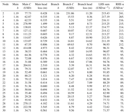
Table 5.Optimization results from Bhave (1978) algorithm. LHS sum and RHS sum are the left and right sides of his Eq. (19), which should be equal.
Node Main MainC Main head Branch BranchC Branch head LHS sum RHS sum
b (USD) loss (m) b (USD) loss (m) (USD m−1) (USD m−1)
2 1.19 77.73 0.428 1.16 231.86 11.20 215.43 241.13
3 1.16 62.87 0.335 1.16 15.53 0.36 217.19 265.77
4 1.16 62.53 0.335 1.16 5.51 5.87 216.11 216.33
5 1.16 278.99 1.499 1.16 6.69 8.73 215.25 215.66
6 1.16 138.01 0.743 1.16 5.13 12.37 214.77 214.60
7 1.16 127.12 0.687 1.16 10.07 17.62 214.12 213.93
8 1.16 111.23 0.603 1.16 9.17 12.31 213.27 213.21
9 1.16 114.87 0.626 1.16 8.87 10.90 212.35 212.13
10 1.16 133.07 0.729 1.16 14.81 14.62 211.19 98.10
11 1.16 67.55 0.806 1.16 69.63 0.70 96.93 212.18
12 1.16 414.08 4.973 1.16 8.42 15.63 96.31 96.70
13 1.16 38.53 0.464 1.16 3.05 14.95 96.07 95.96
14 1.16 64.36 0.778 1.16 4.32 14.63 95.73 95.50
15 1.16 72.08 0.876 1.16 6.67 13.50 95.15 95.33
16 1.16 31.88 0.389 1.16 5.84 17.06 94.76 94.77
17 1.16 204.81 2.510 1.16 5.39 16.31 94.38 93.18
18 1.16 79.31 0.989 1.16 12.07 8.77 92.79 93.44
19 1.16 52.49 0.661 1.16 6.71 8.00 91.85 91.98
20 1.16 88.23 1.121 1.16 6.20 8.28 91.01 91.16
21 1.16 79.12 1.014 1.16 7.47 11.98 90.30 89.01
22 1.16 31.58 0.414 1.16 12.47 7.09 88.29 89.36
23 1.16 51.36 0.680 1.16 8.48 9.99 87.33 85.74
24 1.16 50.84 0.694 1.16 11.52 5.10 84.76 85.51
25 1.16 35.40 0.494 1.16 10.59 6.41 82.90 80.51
26 1.16 29.28 0.431 1.16 20.15 5.27 78.60 82.14
27 1.16 55.92 0.832 1.16 5.52 6.74 77.72 75.66
28 1.16 270.13 4.182 1.16 11.61 4.29 74.71 75.75
29 1.16 222.58 3.545 1.16 8.79 4.42 72.62 73.87
30 1.16 34.71 0.561 1.16 9.56 9.10 71.57 49.43
31 – – – 1.16 47.15 1.13 – –
are omitted since 100 solutions were obtained for each test case. Collectively, the hydraulic grade lines reveal a close alignment of the BT solution (the global optimum) with the CB-Theor solution which utilizes a continuous diameter set. Furthermore, the mapping scheme used to generate a CB-Disc solution is shown to increase pipe sizes in some cases far beyond the limit imposed byhmin, which was set to 7 m
in the present work.
We compared the CB results for the Los Mangos network with those from the Bhave (1978) optimization algorithm (see Table 5). Like Eq. (15) in the present work, Bhave’s op-timality equation (his Eq. 19) equates the sum of a weighted term for all links entering and leaving each internal node in the distribution main. In the present work the term is propor-tional to the hydraulic gradient and the weighting factor is proportional to flow rate. In Bhave’s case the term is the ratio of pipe cost to head loss, where the weighting factor is pipe-cost exponentb. There are 60 nodes for this network, includ-ing 30 nodes in the distribution main. The rest are delivery
nodes (note there are 2 branches from node 30 of the distri-bution main). The terms required for the calculations include b, pipe cost, and head loss in the main and branches. The designation LHS refers to nodes in the distribution main en-tering, and RHS to those leaving, the node at the far-left side of Table 5. The exponentb comes from curve fitting pipe-cost data to the two-part pipe-pipe-cost model. Linear interpola-tion was used between diametersDcoandDco+1to obtainb
in-cluded, which produces additional terms in the optimization equation (see our Eq. 18 above). However, if the system of equations is solved by an iterative method, as Bhave pro-posed, the dependency may be neglected (though issues with convergence of the numerical solution may arise because of this). It is very important to note that if a non-iterative method is used to solve the system of equations as done in the present work (using a commercial program like Mathcad), all terms in the governing equations must be treated as continuous, not discrete, and theb=b(D) dependence must be explicitly in-cluded. It should also be noted that the optimization algo-rithm of Eq. (18) in this paper includes minor loss, which is not included in the Bhave (1978) work.
8 Conclusions
Algorithms to optimize the cost of branching gravity-driven water networks are evaluated on six test cases from real networks in the Philippines, Nicaragua, and Panama. A calculus-based algorithm produced a solution composed of theoretical diameters from a continuous set (CB-Theor), which are then mapped onto discrete commercially available diameters (CB-Disc). Backtracking (BT), a recursive algo-rithm, systematically searches discrete candidate solutions and, when run to completion, is guaranteed to find the global optimum by following rules that prune only higher-cost or hydraulically infeasible candidates. The BT algorithm was modified (BT-NoUp) to improve computational speed by re-jecting all candidates that included a small diameter directly upstream of a larger diameter but allowed for the possibility of missing the global optimum. The third type of algorithm evaluated was a genetic algorithm (GA) that used single-point crossover and tournament selection.
BT could find the global optimum in most test cases with relatively little computational effort, although its poor scaling to larger networks is evidenced by its inability to find a solu-tion to case 6, a network with 60 nodes and 59 links. The BT-NoUp completed its search in less time than BT and could find a solution to case 6. Based on case 1–5 results, the extra pruning condition adopted in BT-NoUp sacrificed only small cost increases. Both BT and BT-NoUp, however, could be-come prohibitively time-consuming when dealing with net-works with significantly more links, diameter choices, or an unfavorable layout. While the test cases represent the range of GDWN sizes encountered in the authors’ experience, fu-ture work would be needed to verify the suitability of the BT and BT-NoUp algorithms on larger GDWNs. The calculus-based algorithm produced consistently good results for the networks tested, although a more robust mapping scheme from theoretical diameters to discrete diameters would fur-ther improve on these results as discussed above. In poten-tial future work, the CB-Theor solutions could be used to prune the BT search space, like Kadu et al. (2008), by only including the two diameters above and below the CB-Theor
diameters, producing four diameter choices per link. The calculus-based methodology provides an additional benefit to the designer by explicitly revealing the sensitivities to cost for a design. The calculus-based algorithm requires greater computational effort than backtracking for smaller networks, however, this effort scales more linearly with the number of network links, while backtracking scales exponentially. Fur-thermore, backtracking’s computational time is sensitive to the number of available diameters. Still, when applied to the present study’s GDWN test cases with a modest number of links (23), backtracking quickly found a global optimum. In addition, because it is guaranteed to find the global op-timum, it can be useful for benchmarking the performance of other algorithms which scale better with more network links. While the genetic algorithm produced solutions with good proximity to the global optimum, its solution costs tended to be further from the global optimum in cases with more links. For all test cases, the calculus-based algorithm’s theoret-ical diameter solutions (CB-Theor) produced a lower cost than the discrete-domain global optimum. This result is made possible because it is not constrained to a discrete set of di-ameters. As such, the CB-Theor results represent a lower-bound on the optimum solution within the problem formu-lation, which could be approached with a finer selection of pipe diameters. We also demonstrated good agreement be-tween the CB-based optimization algorithm developed here and that of Bhave (1978). Though Bhave’s algorithm and Eq. (18) in the present work appear quite different due to the different ways each was developed, both produce optimality for the networks considered in this paper. The key distinc-tion between the two developments is that Bhave assumed exponentbconstant in the pipe-cost model, which was justi-fied based on his iterative method of solution. In the present work, which uses a commercial program to solve the non-linear governing equations forD andh, b(D) dependence is explicitly included for multi-part cost models. Contrasted with Bhave, minor losses are included in the CB optimization algorithm in the present work.
Data availability. All survey data from the network cases tested are available in Table 4.
Competing interests. The authors declare that they have no con-flict of interest.
Acknowledgements. This work was partially supported by the Villanova Undergraduate Research Fellowship Program and the Goldwater Foundation.
Edited by: Luuk Rietveld
References
Alperovits, E., and Shamir, U.: Design of optimal water distribution systems, Water Resour. Res., 13, 885–900, https://doi.org/10.1029/WR013i006p00885, 1977.
Arnalich, S.: How to design a Gravity Flow Water System, Arnalich – Water and Habitat, 2010.
Bhave, P. R.: Optimization of Gravity-Fed Water Distribution Net-works: Theory, J. Environ. Eng.-ASCE, 109, 189–205, 1983. Bhave, P. R.: Non-computer optimization of single source networks,
J. Environ. Eng.-ASCE, 104, 799–814, 1978.
Bhave, P. R.: Optimal design of water distribution networks, Alpha Science International Ltd., Pangbourne, UK, 2003.
Bouman, D.: Hydraulic design for gravity based water schemes, Aqua for All, Den Haag, the Netherlands, 2014.
Churchill, S. W.: Friction factor equation spans all regimes, Chem. Eng. J., 84, 91–92, 1977.
Colebrook, C. F. and White, C. M.: Experiments with fluid fric-tion in roughened pipes, P. R. Soc. London, 161, 367–381, https://doi.org/10.1098/rspa.1937.0150, 1937.
Dandy, G. C., Simpson, A. R., and Murphy, L. J.: An improved genetic algorithm for pipe network optimization, Water Resour. Res., 32, 449–458, https://doi.org/10.1029/95WR02917, 1996. Dongre, S. R. and Gupta, R.: Discussion of ‘Recursive Design of
Pressurized Branched Irrigation Networks’ by César González-Cebollada, Bibiana Macarulla, and David Sallán, J. Irrig. Drain Eng., 138, 697–697, https://doi.org/10.1061/(ASCE)IR.1943-4774.0000441, 2011.
Gessler, J.: Pipe Network Optimization by Enumeration, Proceed-ings of the Specialty Conference on Computer Applications in Water Resources, American Society of Civil Engineers, New York, USA, 572–851, 1985.
González-Cebollada, C., Macarulla, B., and Sallán, D.: Recursive Design of Pressurized Branched Irriga-tion Networks, J. Irrig. Drain Eng., 137, 375–382, https://doi.org/10.1061/(ASCE)IR.1943-4774.0000308, 2011. Jones, G. F.: Gravity-driven Water Flow in Networks: Theory and
Design, Wiley, Hoboken, NJ, USA, 2011.
Kadu, M. S., Gupta, R., and Bhave, P. R.: Optimal design of water networks using a modified genetic algorithm with reduction in search space, J. Water Res. Plan. Man., 134, 147–160, https://doi.org/10.1061/(ASCE)0733-9496(2008)134:2(147), 2008.
Kansal, A., Gupta, R., and Bhave, P. R.: Optimization algorithms for design of branching water distribution networks, J. Indian Water Works Association, 28, 135–140, 1996.
Keedwell, E. and Khu, S.: Novel Cellular Automata Approach to Optimal Water Distribution Network Design, J. Comput. Civil. Eng., 20, 49–56, 10.1061/(ASCE)0887-3801(2006)20:1(49), 2006.
Kessler, A. and Shamir, U.: Analysis of the Linear Pro-gramming Gradient Method for Optimal Design of Wa-ter Supply Networks, WaWa-ter Resour. Res., 25, 1469–1480, https://doi.org/10.1029/WR025i007p01469, 1989.
Krapivka, A. and Ostfeld, A.: Coupled genetic algorithm – Linear programming scheme for least cost design of water distribution systems, J. Water Res. Plan. Man., 135, 298–302, https://doi.org/10.1061/(ASCE)0733-9496(2009)135:4(298), 2009.
Maier, H. R., Simpson, A. R., Zecchin, A. C., Foong, W. K., Phang, K. Y., Seah, H. Y., and Tan, C. L.: Ant colony opti-mization for design of water distribution systems, J. Water Res. Plan. Man., 129, 200–209, https://doi.org/10.1061/(ASCE)0733-9496(2003)129:3(200), 2003.
Martin, Q. W.: Optimal design of water conveyance systems, J. Hydr. Eng. Div.-ASCE, 106, 1415–1433, 1980.
Mohan, S. and Jinesh Babu, K. S.: Water distribution net-work design using heuristics-based algorithm, J. Comput. Civil. Eng., 23, 249–257, https://doi.org/10.1061/(ASCE)0887-3801(2009)23:5(249), 2009.
Monbaliu, J., Jo, J., Fraisse, C. W., and Vadas, R. G.: Computer aided design of pipe networks, Proc. Int. Symp. On Water Re-source Systems Application, Friesen Printers, Winnipeg, Canada, 1990.
Nicklow, J., Reed, P., Savic, D., Dessalegne, T., Harrell, L., Chan-Hilton, A., Karamouz, M., Minsker, B., Ostfeld, A., Singh, A., Zechman, E., and ASCE Task Committee on Evolutionary Com-putation in Environmental and Water Resources Engineering: State of the Art for Genetic Algorithms and Beyond in Wa-ter Resources Planning and Management, J. WaWa-ter Res. Plan. Man., 136, 412–432, https://doi.org/10.1061/(ASCE)WR.1943-5452.0000053, 2010.
Prasad, T. D. and Park, N. S.: Multiobjective genetic algo-rithms for design of water distribution networks, J. Water Res. Plan. Man., 130, 73–82, https://doi.org/10.1061/(ASCE)0733-9496(2004)130:1(73), 2004.
Raad, D. N.: Multi-objective optimisation of water distribution sys-tems design using metaheuristics, PhD thesis, University of Stel-lenbosch, South Africa, 2011.
Saldarriaga, J., Páez, D., Cuero, P., and León, N.: Optimal Design of Water Distribution Networks Using Mock Open Tree Topol-ogy, World Environmental and Water Resources Congress, 19– 23 May 2013, Cincinnati, Ohio, USA, 869–880, 2013.
Samani, H. M. V. and Mottaghi, A.: Optimization of water dis-tribution networks using integer linear programming, J. Hy-draul. Eng., 132, 501–509, https://doi.org/10.1061/(ASCE)0733-9429(2006)132:5(501), 2006.
Simpson, A. R., Dandy, G. C., and Murphy, L. J.: Ge-netic Algorithms Compared to Other Techniques for Pipe Optimization, J. Water Res. Plan. Man., 120, 423–443, https://doi.org/10.1061/(ASCE)0733-9496(1994)120:4(423), 1994.
Streeter, V. L., Wylie, E. B., and Bedford, K. W.: Fluid Mechanics, McGraw-Hill, New York, NY, USA, 1998.
Suribabu, C. R.: Heuristic-based pipe dimensioning model for wa-ter distribution networks, J. Pipeline Syst. Eng., 3, 115–124, https://doi.org/10.1061/(ASCE)PS.1949-1204.0000104, 2012. Swamee, P. K. and Jain, A. K.: Explicit equations for pipe flow
problems, J. Hydr. Eng. Div.-ASCE, 102, 657–664, 1976. Swamee, P. K. and Sharma, A. K.: Gravity low water distribution
network design, J. Water Supply Res. T., 49, 169–179, 2000. Swamee, P. K. and Sharma, A. K.: Design of Water Supply Pipe
Networks, Wiley, Hoboken, NJ, USA, 2008.
Tospornsampan, J., Kita, I., Ishii, M., and Kitamura, Y.: Split-pipe design of water distribution network using simulated anneal-ing, International Journal of Computer, Information, and Systems Science, and Engineering, 1.3, 153–163, 2007.
Vairavamoorthy, K. and Ali, M.: Optimal design of water distri-bution systems using genetic algorithms, Comput. Aided Civ. Infrastruct. Eng., 15, 374–382, https://doi.org/10.1111/0885-9507.00201, 2000.
Vasan, A. and Simonovic, S. P.: Optimization of water distribu-tion network design using differential evoludistribu-tion, J. Water Res. Plan. Man., 136, 279–287, https://doi.org/10.1061/(ASCE)0733-9496(2010)136:2(279), 2010.
Wu, Z. Y. and Walski, T.: Self-adaptive penalty approach compared with other constraint-handling techniques for pipeline optimization, J. Water Res. Plan. Man., 131, 181–192, https://doi.org/10.1061/(ASCE)0733-9496(2005)131:3(181), 2005.
Yang, K. P., Liang, T., and Wu, I. P.: Design of conduit system with diverging branches. J. Hydr. Eng. Div.-ASCE, 101, 167– 188, 1975.
Zhao, W., Beach, T., and Rezgui, Y.: Optimization of Potable Water Distribution and Wastewater Collection Networks: A Systematic Review and Future Research Directions, IEEE T. Syst. Man Cyb., 46, 659–681, https://doi.org/10.1109/TSMC.2015.2461188, 2016.