www.nonlin-processes-geophys.net/16/475/2009/ © Author(s) 2009. This work is distributed under the Creative Commons Attribution 3.0 License.
Nonlinear Processes
in Geophysics
The diffuse ensemble filter
X. Yang and T. DelSole
Center for Ocean-Land-Atmosphere Studies, 4041 Powder Mill Rd., Suite 302, Calverton, MD, 20705, USA George Mason University, Fairfax, VA, USA
Received: 7 May 2008 – Revised: 18 June 2009 – Accepted: 18 June 2009 – Published: 16 July 2009
Abstract. A new class of ensemble filters, called the Dif-fuse Ensemble Filter (DEnF), is proposed in this paper. The DEnF assumes that the forecast errors orthogonal to the first guess ensemble are uncorrelated with the latter ensemble and have infinite variance. The assumption of infinite variance corresponds to the limit of “complete lack of knowledge” and differs dramatically from the implicit assumption made in most other ensemble filters, which is that the forecast er-rors orthogonal to the first guess ensemble have vanishing errors. The DEnF is independent of the detailed covariances assumed in the space orthogonal to the ensemble space, and reduces to conventional ensemble square root filters when the number of ensembles exceeds the model dimension. The DEnF is well defined only in data rich regimes and involves the inversion of relatively large matrices, although this bar-rier might be circumvented by variational methods. Two al-gorithms for solving the DEnF, namely the Diffuse Ensemble Kalman Filter (DEnKF) and the Diffuse Ensemble Trans-form Kalman Filter (DETKF), are proposed and found to give comparable results. These filters generally converge to the traditional EnKF and ETKF, respectively, when the en-semble size exceeds the model dimension. Numerical exper-iments demonstrate that the DEnF eliminates filter collapse, which occurs in ensemble Kalman filters for small ensemble sizes. Also, the use of the DEnF to initialize a conventional square root filter dramatically accelerates the spin-up time for convergence. However, in a perfect model scenario, the DEnF produces larger errors than ensemble square root filters that have covariance localization and inflation. For imperfect forecast models, the DEnF produces smaller errors than the ensemble square root filter with inflation. These experiments suggest that the DEnF has some advantages relative to the ensemble square root filters in the regime of small ensemble size, imperfect model, and copious observations.
Correspondence to: X. Yang
1 Introduction
It is well established that forecast ensembles in ensemble-based Kalman filters tend to collapse – that is, the forecast spread tends to shrink with time until the filter effectively re-jects the observations.1The collapse of the ensemble implies that the forecast errors are underestimated and that the filter weights the first guess too heavily. Eventually, the forecast becomes so “overconfident” that the filter ignores the obser-vations altogether. Two methods for avoiding filter collapse are covariance inflation (Anderson and Anderson, 1999) and localization (Hamill et al., 2001; Houtekamer and Mitchell, 2001). Covariance inflation attempts to avoid filter collapse by inflating the covariance of the ensemble by an empirical factor. However, covariance inflation alone cannot prevent filter collapse if the ensemble size is sufficiently small, as we will show. This result may be understood as follows. The full state space can be split into two subspaces: the space spanned by the ensemble, which we call the ensemble space, and the complement to the ensemble space, which we call the null space. Generally for atmospheric applications, the ensem-ble size is much less than the model dimension, so that the ensemble does not span the full model space, and hence the null space is very large. In essence, the ensemble filters, e.g., the ensemble Kalman filter (EnKF) (Evensen, 1994) and en-semble square root filters (Tippett et al., 2003), updates only those variables in the ensemble space. It follows that vari-ables in the null space are not updated, which is equivalent to assuming that the forecast covariance of the null space vec-tors vanishes. Thus, no matter how much inflation is applied,
1Some papers refer to this phenomenon as filter divergence. For
this inflation only influences the ensemble space, leaving the variances in the null space zero and hence underestimated.
The above reasoning highlights a very unrealistic property of ensemble filters: they effectively assume that forecast er-rors in the null space vanish. Consequently, observations have no impact on the null space, regardless of how much the ensemble is inflated. This deficiency of ensemble filters deserves emphasis: if the ensemble size is small but the ob-servations are abundant, the obob-servations nevertheless are not used to modify the ensemble outside the space spanned by the first guess, no matter how many observations are avail-able that would justify such modifications. This deficiency follows directly from the assumption that the forecast is “per-fect” in the null space, an assumption that is grossly incorrect for atmospheric and oceanic data assimilation, in which the underlying forecast model is imperfect. The question arises as to whether a Kalman filter can be formulated in such a way as to avoid the assumption of vanishing forecast errors in the null space. In an abstract sense, a similar situation occurs in the initialization of a Kalman filter – the forecast covari-ance matrix generally is not available at the first time step. To deal with incompletely specified initial conditions, Ans-ley and Kohn (1985) proposed a method that is equivalent to assuming a diffuse prior distribution for the unspecified part of the initial state. A distribution is said to be diffuse if its covariance matrix is arbitrarily large (de Jong, 1991). The diffuse assumption often corresponds to the limit of com-plete lack of knowledge in Bayesian analysis, from which the Kalman filter can be derived (Maybeck, 1979). Ansley and Kohn (1985) and de Jong (1991) discuss the extension of the Kalman filter to partially diffuse covariance matrices.
The purpose of this paper is to develop an extension of ensemble filters to allow for arbitrarily large forecast errors. Our fundamental assumption is that the forecast errors or-thogonal to the ensemble are uncorrelated with the errors in the ensemble, and are infinitely large. We call the resulting filters Diffuse Ensemble Filters (DEnFs). We propose two specific algorithms called the Diffuse Ensemble Kalman
Fil-ter (DEnKF) and the Diffuse Ensemble Transform Kalman Filter (DETKF). Our derivation of the DEnFs is essentially
independent of Ansley and Kohn (1985) and de Jong (1991), as it is tailored to the special needs of an ensemble Kalman filter. It should be recognized, however, that the derivation of a diffuse filter is subtle. For instance, the filtering and limiting operations are not interchangeable, as noted by Ans-ley and Kohn (1985). Also, early derivations of diffuse fil-ters were numerically inefficient. In the derivation presented here, the proof is general, direct, and yields a closed form set of equations.
Another approach to avoiding filter collapse is covariance localization. Covariance localization attempts to reduce the spurious correlations that inevitably arise from sample based estimates by taking the Schur product between the sample based estimate and a distance-dependent function that varies from unity at the observation location to zero at some
pre-defined radial distance. In order to maintain the positive definiteness of covariance matrices, the distance-dependent function used in the Schur product must itself be positive def-inite. This procedure can be interpreted as imposing structure on the error covariance, in which case the ensemble effec-tively gives information about many more degrees of free-dom than just the ensemble space. Accordingly, covariance localization changes the rank of the forecast covariance; in particular, it usually eliminates the null space (as we will show). Thus, there can be no diffuse ensemble filters with lo-calization, because under localization there is no null space for applying the diffuse assumption. However, localization alone still allows underestimation of covariances and hence most applications of covariance localization also apply co-variance inflation.
The paper is organized as follows. The algorithm of DEnFs is presented in Sect. 2, and the experimental setup is described in Sect 3. Data assimilation experiments with the Lorenz 96 model are used to compare the diffuse ensem-ble filters and the ensemensem-ble filters in Sect. 4. Initialization using DETKF is presented in Sect.5. The paper ends with the conclusions and discussions in Sect. 6.
2 Derivation of the Diffuse Ensemble Filters
In this section we review traditional ensemble filters, use a simple example to illustrate some differences between dif-fuse and traditional filters, and then derive the Difdif-fuse En-semble Kalman Filer (DEnKF) and the Diffuse EnEn-semble Transform Kalman Filter (DETKF). We end this section by discussing additional generalizations of the diffuse filter. 2.1 The Ensemble Transform Kalman Filter (ETKF)
The Ensemble Transform Kalman Filter (ETKF) was pro-posed by Bishop et al. (2001) and clarified by Tippett et al. (2003). We briefly review this filter to establish notation and provide a reference for comparison. The standard Kalman Filter equations for the mean update and the analysis covari-ance matrix are (Maybeck, 1979, p117)
¯
9a = ¯9f +PHT R+HPHT −1
o−H9¯f (1) Pa =P−PHT R+HPHT
−1
HP, (2)
where9¯ is the mean state vector, R is the observation
er-ror covariance matrix, H is the observation operator, P is the forecast covariance matrix, andois the observation vector. Let the difference between thej-th ensemble member and the ensemble mean be denoted by the M-dimensional vector
aj. For ensemble sizeN, let
A=√ 1
Then an unbiased estimate of the forecast covariance matrix is
PE =AAT. (4)
The ensemble Kalman Filter is obtained by substituting the sample covariance matrix PEfor P in (1) and (2). By
invok-ing the Sherman-Morrison-Woodbury formula, it is straight-forward to show that the resulting analysis covariance matrix can be written as
Pa=AI+ATHTR−1HA −1
AT. (5)
An analysis ensemble matrix Aasuch that Pa=Aa(Aa)T is derived by setting
Aa=AI+ATHTR−1HA −1/2
, (6)
where the matrix in parentheses is a square root matrix. The square root matrix can be derived by computing the eigen-vector decomposition
I+ATHTR−1HA=YDYT, (7)
where Y is unitary and D is a diagonal element with positive diagonal elements, and then setting
I+ATHTR−1HA −1/2
=YD−1/2YT. (8) As noted by Sakov and Oke (2008), the symmetric form of the square root defined in (8) preserves the ensemble mean.
We draw attention to the following fact. It is evident that the mean update is pre-multiplied by A, and that the covari-ance update is pre- and post-multiplied by A and AT, respec-tively. It follows that the mean and covariance updates occur only in the subspace spanned by the first guess ensemble. Therefore, the ensemble Kalman Filter does not modify any variable in the space orthogonal to the ensemble. This result is tantamount to assuming that the forecast covariance matrix vanishes in the null space, which of course is highly unreal-istic, and the filter is overconfident in the null space. As we will see, this characteristic of the ensemble square root filter (ESRF) distinguishes it from the diffuse filter.
2.2 A simple example
In this section, we present a simple 2-dimensional example to illustrate some key properties of various filters. Without loss of generality we use a basis set in which the forecast covariance matrix is diagonal:
P=
pE 0
0 pN
. (9)
Shortly, we will interpret pE as the variance in ensemble
space and pN as the variance in the null space. Consider
the situation in which only two observations are available. Although general observation networks can be considered, this extra generality does not lead to substantial insights in this 2-D problem. Accordingly, we make the simplifying as-sumptions that H and R are diagonal:
H=
1 0 0 1
R=
rE 0
0 rN
. (10)
The mean analysis under these assumptions is
¯
9a = ¯9f +PHT R+HPHT −1
o−H9¯f (11)
= ¯
9Ef
¯
9Nf !
+ pE pE+rE 0
0 pN
pN+rN
!
oE− ¯9Ef
oN− ¯9Nf
!
(12)
=
¯
9Ef + pE pE+rE
oE− ¯9Ef
¯
9Nf + pN pN+rN
oN− ¯9Nf
, (13)
where the mean forecast is denoted9¯f =(9¯f E 9¯
f N)
T.
Sim-ilarly, the covariance matrix update is Pa=P−PHT HTPH+R
−1
HP (14)
=
pE−
pE2
rE+pE 0
0 pN−
p2 N rN+pN
. (15)
Let us first consider the Kalman Filter solution for an en-semble size of two. In this case, the forecast covariance ma-trix is rank-1. IfpE is identified as the variance of the
en-semble, thenpN=0. The mean update in this case is ¯
9a = ¯
9Ef + pE pE+rE
oE− ¯9Ef
¯
9Nf
!
, (16)
while the covariance update is
Pa= pE− p2E rE+pE 0
0 0
!
(17) This solution reveals two key characteristics of the ensemble based Kalman Filter: the analysis increment (i.e.,9¯a− ¯9f) is confined to the ensemble space, and the covariance matrix update (i.e., Pa−P) is confined to the ensemble space. This means that the forecast in the null space is not modified; that is,9¯Na= ¯9Nf. The limit pN→0 implies that the forecast in
the null space has zero uncertainty, or equivalently that the forecast is “perfect.” This assumption is obviously unrealis-tic in genuine data assimilation problems in which nature is unknown.
Let us now consider the diffuse limit, which corresponds to the limitpN→∞. This limit is easily evaluated as
¯
9a = ¯
9Ef + pE pE+rE
oE− ¯9Ef
oN
!
and
Pa=
1
1 rE+
1 pE
0 0 rN
!
. (19)
The solution shows that the update in ensemble space is ex-actly the standard KF solution, while the update in the null space is replaced by the appropriate observation. This result is sensible, since the diffuse limit implies that the forecast is completely uncertain and so the analysis should reduce to the observation. In contrast to the ensemble based Kalman Filter, the update occurs in both the ensemble space and the null space.
2.3 The Diffuse Ensemble Filter
The basic assumption in the DEnFs is that the forecast errors orthogonal to the first guess ensemble are uncorrelated with the ensemble and have infinite covariance matrix. With this assumption, we will derive the algorithm to update the en-semble using the Kalman Filter. Let the SVD of theM×N matrix A be
A=USVT, (20)
where S is anM×N diagonal matrix, whose diagonal ele-ments specify the non-negative singular values, ordered from the largest to smallest, and U and V are unitary (but having respective dimensionsM×MandN×N). At most,N −1 diagonal elements of SSTare nonzero, since the ensemble mean has been subtracted from each member. Assume that exactlyN−1 singular values are nonzero. Furthermore, let the singular vectors be ordered such that the firstN−1 vec-tors are those with non-zero singular values. This ordering allows us to partition the singular vector matrix U as
U=UE UN, (21)
where UEdenotes theM×(N−1)matrix whoseN−1 col-umn vectors are the singular vectors associated with non-zero singular values, and UNdenotes the matrix containing the re-maining singular vectors that span the null space. The fore-cast ensemble covariance matrix can then be written as PE=UESSTUTE=UES2EUTE (22) where SEis anN −1 dimensional, square, diagonal matrix whose diagonal elements equal the non-zero singular values of A.
To derive the diffuse ensemble filter, we start with the “in-verse” form of the Kalman filter equations (Maybeck, 1979, Sect. 5.7), also known as the information filter, which are
¯
9a= ¯9f+HTR−1H+P−1 −1
HTR−1o−H9¯f (23) Pa=HTR−1H+P−1
−1
. (24)
Since PEis not invertible, we cannot simply substitute P=PE in these equations as we did for the standard form of the Kalman filter equations. Accordingly, we invoke a fictitious ensemble whose covariance matrix is PNsuch that total fore-cast covariance
P=PE+PN (25)
is nonsingular. The first assumption of the diffuse filter is that PEand PN are orthogonal; i.e., PEPN = PNPE = 0. This implies that PNis of the form
PN=UN6UTN (26)
where6 is a nonsingular matrix specifying the covariance matrix in the null space. Under this assumption the inverse forecast covariance matrix becomes
P−1=U
S−E2 0 0 6−1
UT. (27)
The second assumption of the DEnFs is that6−1→0. One way to interpret this limit is to define PN=αUN60UTN, where
60is a constant, nonsingular matrix, and then take the limit α→∞. In this case,6−1→0 regardless of the detailed struc-ture of60; that is, the limit is independent of the details of the forecast covariance in the null space. The diffuse limit is therefore
P−dif1=U
S−E20 0 0
UT=UES−E2UE. (28)
The substitution P−1→P−dif1in (23) and (24) may present problems because the matrix HTR−1H+P−1may be singu-lar and therefore has no inverse. We show in the appendix that a necessary and sufficient condition for Pato be nonsin-gular is that the auxiliary matrix
W=UTNHTR−1HUN (29)
should be nonsingular. The restriction that W be invertible can be interpreted as requiring that the observations project onto every degree of freedom in the null space. Loosely speaking, if W is singular, then there exists a vector in the null subspace that is unobserved. This restriction is sensible in light of the fact that the null space has no model infor-mation under the diffuse assumption, so the only other in-formation available for updating the null space must come from observations. Since Pa is nonsingular in this case, it is full rank, indicating that the mean and covariance updates are not confined to the ensemble subspace. This represents a fundamental difference with other ensemble Kalman Filters. To summarize, the mean update equation for the DEnF is
¯
9difa = ¯9f+HTR−1H+P−dif1 −1
and the covariance update, derived by substituting (28) into (24), is
Pa=HTR−1H+UES−E2U T E
−1
. (31)
The fact that Pais full rank when W is full rank raises the question as to how to define an analysis ensemble. This ques-tion does not arise in tradiques-tional EnKFs because the analysis and forecast span exactly the same space and hence can be represented by the same number of basis vectors. In con-trast, the DEnF may start with a small ensemble but leads to a full rank analysis covariance matrix that cannot be rep-resented by an ensemble size smaller than or equal to the model dimension. Of the many approaches to deriving an ensemble filter that can be conceived, we present two: one based on perturbed observations, and one based on project-ing the analysis into the ensemble space. At the end of this section we discuss alternative solution methods, including a method that relaxes the requirement that W be nonsingular. 2.3.1 The Diffuse Ensemble Kalman Filter (DEnKF)
Houtekamer and Mitchell (1998) and Burgers et al. (1998) proposed what is now called the Ensemble Kalman Filter (EnKF), which is characterized by randomly perturbed ob-servations. By analogy, we propose the Diffuse Ensemble Kalman Filter (DEnKF), in which the ensemble update for thei-th ensemble member is defined as
9ia=9if+HTR−1H+UES−E2UTE −1
HTR−1oi−H9if
, (32) where i = 1, . . . , N, oi = o +ri, ri ∼ N(0,R), and N(µ, σ2) denotes a Gaussian distribution of mean µ and varianceσ2. If the forecast covariance matrix based on the ensemble is full rank, UNequals 0, and the DEnKF reduces
to the EnKF. Note that the analysis increment9if−9afof the
DEnKF is not restricted to the ensemble space, in contrast to the EnKF.
2.3.2 The Diffuse Ensemble Transform Kalman Filter (DETKF)
A deterministic diffuse filter can be derived by analogy with the ETKF (see Sect. 2.1). In this case, the mean update is given by the same equation as in the ETKF, namely (30). However, instead of using the full analysis covariance (31), we project Paonto the ensemble space. This projection im-plies that the ensemble is updated only in the space spanned by the first guess ensemble, just as in the ETKF. We show in the appendix that the final analysis update equation for the DETKF is
Padif=A h
I+ATHT
R−1−R−1HUNW−1UTNHTR
−1HAi−1AT. (33) Comparison of this equation with (5) reveals that the DETKF differs from the ETKF by an extra term in the matrix whose
inverse is taken. Furthermore, this extra term has the effect of inflating the analysis ensemble (i.e., Padif−Pais positive
semi-definite). This inflation reflects the fact that the DETKF accounts for uncertainty in the null space, whereas the ETKF effectively assumes the forecast in the null space is perfect. The DETKF and ETKF become identical if
UTEHTR−1HUN =0, (34)
because in this case the “extra” term in (33) vanishes. It is sensible that the DETKF and ETKF have the same ensem-ble spread when (34) is satisfied, because the observations in the ensemble space and null space are uncorrelated, in which case observations in the null space provide no information for updating the ensemble space.
The square root form of the DETKF is obtained by solving the eigenvalue decomposition
I+ATHT
R−1−R−1HUNW−1UTNHTR
−1HA=YDYT, (35) where Y is unitary and D is a diagonal matrix with positive diagonal elements, and then defining
Aadif=AYD−12YT, (36)
which gives Padif = Aadif(Aadif)T. If ensemble covariance is full rank, UN equals 0, and the DETKF reduces to the
En-semble Transform Kalman Filter (ETKF). Thus, the DETKF does not converge to the ensemble square root filter (ESRF) of Whitaker and Hamill (2002) as ensemble covariance goes to full rank, since the latter filter differs from the ETKF. 2.4 Alternative diffuse filters
We emphasize that the DEnKF and DETKF require invert-ing matrices of the order of the model dimension. For atmo-spheric and oceanic models, this dimension can easily exceed 100 000, which is clearly impractical. However, the DEnKF might be solvable using an equivalent variational method, just as large scale data assimilation problems are solved us-ing variational methods at operational centers (Klinker et al., 2000). As is well known (Maybeck, 1979, p. 234), the mean update of the Kalman Filter equations minimizes the cost function
L= o−H9¯T
R−1 o−H9¯ +
¯
9−9¯fTP−19¯−9¯f. (37) The first term can be interpreted as a “goodness of fit”, since it measures how close the state is to the observations, while the second term is a penalty function, since it increases with the distance between the state and first guess. Under the dif-fuse assumption, this cost function becomes
L= o−H9¯T
R−1 o−H9¯
+UTE9¯−9¯fT
S−E2UTE9¯−9¯f
. (38)
advantage of minimizing this cost function is that it can be solved with standard conjugate gradient methods without ex-plicitly inverting the matrix W. Unfortunately, the resulting solution gives only the mean update; how one can use (37) and (38) to generate an ensemble filter is unclear.
Another question is whether the restriction that W be non-singular can be relaxed. One theoretical barrier to defining a diffuse limit when W is singular is that it leads to a contra-dictory situation. Specifically, singular W implies that nei-ther the forecast ensemble nor the observations constrain a certain space. Indeed, it is possible to show that L is in-dependent of the null vectors of W, indicating thatL does not constrain these vectors. Now, if neither the forecast nor the observations constrains part of the null subspace, then on what basis can one update this space? The solution to this problem is to apply the diffuse assumption only to the part of the null space that is constrained by observations. This can be accomplished by splitting the null space itself into two parts, one constrained by observations (identified by the range of W), and one unconstrained by observations (identi-fied by the null space of W). Then, the diffuse assumption can be applied to the subspace that is constrained by observa-tions, while the “perfect model” assumption can be applied to the subspace that is unconstrained by observations. This alternative diffuse filter will not be discussed further in this paper.
3 Experimental setup
The model used here is the Lorenz-96 model (Lorenz and Emanuel, 1998), which is governed by the equation
dxi
dt =(xi+1−xi−2) xi−1−xi+f0, (39) wherei = 1. . . J with cyclic indices. Here, J is 40 andf0
is 8.0. The consecutive model states are obtained by inte-grating the model forward with the time interval 0.05, and a fourth-order Runge-Kutta numerical method is applied at each model time step. The truth is one single integration of the model. The observational data set was constructed by adding Gaussian white noise with zero mean and unit vari-ance to the truth at each of the 40 grid points, thereby pro-ducing 40 observations at each time step.
In realistic data assimilation, the model is imperfect due to model errors, e.g., uncertain model parameters. In this study, we will conduct some data assimilation experiments with an imperfect model, defined as
dxi
dt =(xi+1−xi−2) xi−1− xi
1.0+di
+f0+fi, (40)
where the dissipation parametersdi and forcing parameters
fiare randomly specified according to
fi ≈N (0,4), i=1. . . J, (41) di ≈N (0.5,0.5), i=1. . . J. (42)
The ensemble filters used here are the EnKF of Evensen (1994) and the ESRF of Whitaker and Hamill (2002). The initial ensemble members for the first data assimilation ex-periment are generated by adding independent, zero mean, normally distributed random numbers of variance 1.0 to the climatology of the long run with 30 000 time steps. The co-variance inflation for all experiments in this study, when ap-plied, is the adaptive covariance inflation algorithm proposed by Anderson (2007) or constant inflation (Anderson and An-derson, 1999). The localization applied here is the fifth or-der polynomial function of Gaspari and Cohn (1999) with half-width c. Localization half widthcis 10 relative to the model domain size 40. If the distance between the observa-tion and the state variable is greater than 2c, then the localiza-tion funclocaliza-tion is zero, which implies that the observalocaliza-tion has no impact on the state variable; otherwise, it approximates a Gaussian. The root mean square error (RMSE) is computed as the root mean square of the difference between the analy-sis and the truth over the 40 grid points and from model time steps 3000 to 6000.
To test the consistency between observations and filter out-put, we use the fact, as noted by (Maybeck, 1979, p229), that the Kalman filter predicts that the innovation vector
z=o−H9¯f (43)
is a white Gaussian sequence with zero mean and covariance matrix
C=HPHT +R. (44)
This fact allows us to construct an innovation consistency
function (ICF). Specifically, if this assumption is correct,
then the quadratic form
ICF=zTC−1z (45)
4 Numerical results
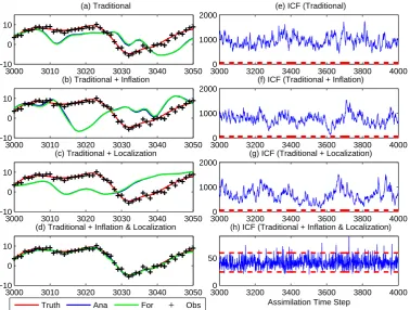
Figure 1a–d shows a typical result for the truth, observation, forecast, and analysis by the ensemble square root filter at one grid point in the Lorenz-96 model. Note that the blue and green curves are superposed and undistinguishable. The innovation consistency function (ICF) is shown in Fig. 1e–h (for a longer time period). Note that the two ICF thresh-olds in panels e, f, and g are undistinguishable since ICFs are much larger than the two thresholds. Inspection of Fig. 1e–h shows that the innovations are consistent with the filter only if both covariance inflation and localization are applied (i.e., the ICF lies between the two dashed lines only in Fig. 1h). In other cases, the innovations are inconsistent with the fil-ter. More importantly, the ensemble collapses in the cases illustrated in Fig. 1a–c – the analysis is weighted too heavily toward the model forecast, allowing the analysis to diverge from the observations. Interestingly, the ensemble square root filter with just localization still diverges (Fig. 1c and g) even though there is no null space. This may be due to the model non-linearity and underestimation of covariances by the sample ensemble.
The results for the DETKF are shown in Fig. 2a and c. The figures show that the amplitudes of the innovation vec-tors produced by the DETKF are too large relative to that assumed internally by the filter. However, in this case, there is no ensemble collapse. Instead, the analysis is weighted too heavily to the observations. Consequently, the analysis reveals much more high frequency noise than the truth, ow-ing to the white noise in the observations. Just as with the ensemble filters, the DETKF might be improved with covari-ance inflation. Accordingly, we apply covaricovari-ance inflation to the forecast ensemble (we do not inflate the null space co-variances, since they are already inflated by the diffuse limit assumption). The ICF when covariance inflation is applied to the DETKF is shown in Fig. 2d, which reveals that inflation does indeed improve the consistency. It turns out that infla-tion also improves the RMSE of the analysis (not shown).
In order to avoid ensemble collapse due to the finite en-semble size and model non-linearities, two common meth-ods, covariance inflation (Anderson and Anderson, 1999) and localization (Hamill et al., 2001; Houtekamer and Mitchell, 2001), are usually applied. The diffuse limit can be interpreted as an extreme example of inflation for the null space. Yet, even with infinite covariances in the null space, the diffuse filter still diverged. Similarly, in the ESRF with localization, there is no null space, yet the filter still diverges. Thus, an interesting conclusion from the above results is that the filter converges only when the covariance of both the en-semble space and the null space are inflated – inflating just one subspace is not enough to avoid filter collapse.
Covariance localization can not be implemented in the dif-fuse ensemble filters because it usually eliminates the null space by rendering the forecast covariance matrix full rank. Figure 3 shows the minimum spectrum of eigenvalues of the
forecast covariance matrix for 10 ensemble members with and without covariance localization. Without localization, the covariance matrix has 9 nonzero eigenvalues and 31 zero eigenvalues, which corresponds to the size of the ensem-ble space and null space respectively. All eigenvalues are nonzero when the covariance localization is applied, which implies that the localized covariance matrix is full rank and hence the null space is zero. The eigenvalue spectrum slope is deeper when the localization half width is larger. Note that covariance localization also intends to reduce sampling errors.
To investigate the sensitivity of the results to ensemble size, we show in Fig. 4a the performance of the ESRF and the DETKF, with inflation, as a function of ensemble size. For the ensemble size 41, there is no null space, so the DETKF is identical to the ETKF, and the values of RMSE for the two filters are almost the same (the small difference arises from the fact that the ESRF of Whitaker and Hamill (2002) differs from the ETKF). We see that the RMSE for the ESRF de-creases dramatically and eventually the filter converges after 15 ensemble members. This implies that inflation alone can allow the filter to converge if the ensemble size is sufficiently large. Equivalently, if the ensemble size is too small, then inflation alone is not enough to prevent filter collapse. Thus, for small ensemble sizes relative to the model dimension, the DETKF may be an attractive alternative to the ETKF.
One can argue that the above test is not completely fair because the dynamical model is perfect in the sense that it is identical to the model that generates the truth. Conse-quently, the first guess of the dynamical model is very good, and therefore a filter that reduces to the first guess in the null space may perform preferentially better than a filter that does not. Accordingly, we consider a new test by using the imper-fect model (40) to generate forecasts, but use the same set of observations generated by the original model (39). Note that the adaptive covariance inflation tends to be larger in the imperfect model case to account for model errors (Ander-son, 2007). The resulting average RMSE as a function of ensemble size is shown in Fig. 4b. Compared to the perfect model scenario, the performance of the ESRF is dramatically degraded, especially for small ensemble sizes, while the per-formance of DETKF does not change much. This implies that DETKF outperforms the ESRF without localization for the imperfect model scenario.
3000 3010 3020 3030 3040 3050 −10
0 10
(a) Traditional
3000 3010 3020 3030 3040 3050
−10 0 10
(b) Traditional + Inflation
3000 3010 3020 3030 3040 3050
−10 0 10
(c) Traditional + Localization
3000 3010 3020 3030 3040 3050
−10 0 10
(d) Traditional + Inflation & Localization
Truth Ana For Obs
30000 3200 3400 3600 3800 4000
1000 2000
(e) ICF (Traditional)
30000 3200 3400 3600 3800 4000
1000 2000
(f) ICF (Traditional + Inflation)
30000 3200 3400 3600 3800 4000
1000 2000
(g) ICF (Traditional + Localization)
30000 3200 3400 3600 3800 4000
50
(h) ICF (Traditional + Inflation & Localization)
Assimilation Time Step
Fig. 1. Time series based on the Lorenz 96 model of the truth (red), the model forecast (green), the analysis (blue) and the observation (plus)
at one grid point for (a) ESRF without inflation and localization, b) ESRF with inflation only, c) ESRF with localization only, and d) ESRF with localization and inflation. Time series of the innovation consistency function (ICF) for e) ESRF without inflation and localization, f) ESRF with inflation only, g) ESRF with localization only, h) ESRF with localization and inflation. Ensemble size is 10 for all experiments. Localization half widthcis 10 relative to the model domain size 40. Red dashed line indicating the threshold value of ICF.
3000 3010 3020 3030 3040 3050
−10 −5 0 5 10 15
(a) DETKF
Tru Ana For Obs
3000 3010 3020 3030 3040 3050
−10 −5 0 5 10 15
(b) DETKF with inflation
Assimilation Time Step
30000 3200 3400 3600 3800 4000
50 100 150
(c) ICF of DETKF
30000 3200 3400 3600 3800 4000
5 10 15 20 25
(d) ICF of DETKF with inflation
Assimilation Time Step
Fig. 2. Time series based on Lorenz 96 model of the truth (red), the model forecast (green), the analysis (blue) and the observation (plus) at
0 5 10 15 20 25 30 35 40 10−10
10−5 100
Eigenvalue nummber
Magnitude
Minimum Eigenvalue Spectrum with/without Localization
10 ensembles + Localization (c=10) 10 ensembles + Localization (c=20) 10 ensembles; No Localization
Fig. 3. Minimum of the ordered eigenvalues of the forecast
covari-ance matrix for 10 ensemble members with and without covaricovari-ance localization. The minimum is obtained from assimilation time steps 3000 to 6000, and localization was applied forc=10 andc=20, as indicated in the figure. Note that all 31 zero eigenvalues for 10 en-semble members without localization are set to 10−10 for plotting purpose.
observations in both EnKF and DEnKF degrade the perfor-mance of filters. This is the reason that in this study we focus on the performance of DETKF, rather than DEnKF.
5 Initialization using DESRF
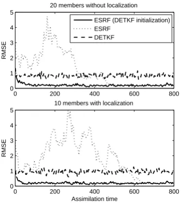
Originally, the diffuse Kalman filter was designed to initial-ize the Kalman filter (de Jong, 1991; Koopman, 1997). Anal-ogously, DETKF can be applied to initialize the ESRF. Here, we first run the DETKF for one time step to get the analyzed ensemble mean and perturbations, and then these optimal en-semble members are used to initialize the ESRF. Note that in this section the root mean square error (RMSE) is defined as the root mean square of the difference between the analysis and the truth over the 40 grid points. Figure 6a shows the RMSE as a function of assimilation time for the ESRF with and without using DETKF initialization with 20 ensemble members. The ESRF with standard initial ensembles of ran-dom Gaussian noise perturbations converges slowly to the optimal level of RMSE at around 500 assimilation time steps, while the ESRF, initialized with DETKF, converges rather quickly to the optimal level of RMSE at round 50 assimila-tion time step. After 500 assimilaassimila-tion time step, the RMSEs of these two different ensemble initializations are indistin-guishable. The same experiment with 10 ensemble members plus localization reveals the similar results (Fig. 6b). This implies that initialization using DETKF accelerates the ini-tial spin-up time for the ESRF.
6 Summary and discussion
This paper proposed a new type of filter called the Diffuse Ensemble Filter (DEnF). The DEnF assumes that the forecast errors in the space orthogonal to the first guess ensemble are
5 10 15 20 25 30 35 40 0
1 2 3
RMSE (Perfect Model)
(a) DETKF
ESRF
5 10 15 20 25 30 35 40 0
1 2 3
Ensemble Size RMSE (Imperfect Model)
(b) DETKF
ESRF
Fig. 4. The root mean square error (RMSE) as a function of
en-semble size for the ESRF with inflation (dashed) and the DETKF with inflation (solid) using the (a) perfect and (b) imperfect mod-els. Results are averaged over the 3000 to 6000 assimilation time step.
5 10 15 20 25 30 35 40 0
1 2 3
(a) EnKF
DEnKF
5 10 15 20 25 30 35 40 0
0.5 1 1.5
(b) DETKF
DEnKF
Fig. 5. The root mean square error (RMSE) as a function of
en-semble size for (a) the EnKF with inflation (solid) and the DEnKF with inflation (dashed), (b) the EnKF with inflation (dashed) and the DETKF with inflation (solid) using the perfect model. Results are averaged over the 3000 to 6000 assimilation time step.
uncorrelated with the latter ensemble, and are infinite, corre-sponding to complete lack of information. Thus, in terms of the forecast covariance matrix in the null space PN, ensemble
filters assume PN→0, while diffuse filters assume PN→∞.
0 200 400 600 800 0
1 2 3 4 5
20 members without localization
RMSE
ESRF (DETKF initialization) ESRF
DETKF
0 200 400 600 800
0 1 2 3 4 5
10 members with localization
RMSE
Assimilation time
Fig. 6. The root mean square error (RMSE) between analysis and
truth as a function of assimilation time for the ESRF with DE-TKF initialization (solid) and with random initial conditions (dot-ted) using (a) 20 ensemble members plus constant inflation and
(b) 10 ensemble members plus constant inflation and localization.
RMSE of DETKF (dashed) is plotted for reference. The inflation factor is 1.08 for (a), and 1.05 for (b).
to apply the diffuse assumption. The diffuse limit is well de-fined only in observation rich regimes (more precisely, the matrix W defined in (29) is invertible). In the null space, the analysis produced by the DESRF is strongly coupled to the observations, consistent with assuming infinite forecast covariance in this space, whereas the analysis produced by traditional filters is strongly coupled to the first guess.
Numerical experiments presented in this paper demon-strate that the DETKF and DEnKF successfully prevent filter collapse for small ensemble sizes. Unfortunately, the ampli-tude of the innovation vectors produced by these filters are too large relative to that assumed internally in the filters. In addition, the analyses produced by the diffuse filters have significantly larger error than those produced by the ESRF with inflation and localization. Inflating the ensemble fore-cast covariance in the DETKF reduces the analysis errors, but does not reduce them as much as the ESRF with inflation and localization. To investigate the impact of using an imper-fect forecast model, we conducted assimilation experiments using a forecast model in which the forcing and dissipation parameters were perturbed relative to the model that gener-ated the truth. We found that the performance of the ESRF was significantly degraded by the presence of model errors, whereas the DETKF was not since it is less dependent on the first guess. These results suggest that the DETKF can outperform ESRF without localization in the more realistic case of small ensemble size and imperfect model, provided enough observations are available to render a well defined diffuse limit.
The DETKF also was found to dramatically accelerate the spin-up time of the ESRF. This result is consistent with the study of Zupanski et al. (2006), who found that the com-monly used initial ensemble of uncorrelated random pertur-bations for the ESRF converged slowly, while initial per-turbations that had horizontally correlated errors converged faster. Kalnay and Yang (2009) also found that the spin-up time of EnKF is longer than the corresponding spin-spin-up time in variational methods, and they proposed a scheme to accelerate the spin-up of EnKF applying a no-cost Ensem-ble Kalman Smoother, and using the observations more than once in each assimilation window in order to maximize the initial extraction of information. We note that the DETKF still requires a guess for the initial condition and error co-variances, unlike the diffuse Kalman filter (de Jong, 1991; Koopman, 1997).
A fundamental limitation of the DEnFs, as formulated here, is that it requires a relatively large number of obser-vations. The precise condition is that the matrix W defined in (29) needs to be invertible. For this operator to be in-vertible, the observations must be sufficiently numerous as to constraint the analysis in the null space. This constraint is a natural consequence of the diffuse assumption – since the forecast is completely uncertain in the null space, the only other information available for specifying the assimilation is the observations. That is, if neither the forecast nor observa-tions are available in the null space, then there is no basis for estimating the corresponding state. With the emergence of copious data from satellites, this constraint might be satisfied for realistic atmospheric data assimilation. It is possible to generalize the DEnFs to situations in which W is singular, but this approach was only outlined in this paper.
The limitation that W be invertible is not only a theoreti-cal limitation of diffuse filters, but also a practitheoreti-cal limitation, because the dimension of this matrix is approximately equal to the model dimension minus the ensemble size. For atmo-spheric or oceanic models, this dimension can easily exceed 100 000, which is clearly impractical at the present time. We briefly described a variational solution for the DETKF that avoids inversion of W.
The fact that diffuse filters do not perform as well as the ESRF with inflation and localization is instructive. In the DETKF, the covariances in the null space are inflated while the covariances in the ensemble space are not. Conversely, in the ESRF with inflation only, the covariances in the ensem-ble space are inflated while the covariances in the null space are not. Neither case produces as good an analysis as the ESRF with both inflation and localization. Presumably, the benefits of localization derive from the fact that the forecast errors of the system actually do have spatially local corre-lations. In other words, the first guess ensemble really does contain information about the null space, even though it is or-thogonal to it. It would be interesting and more consistent to develop a filtering scheme that imposes this structure in the prior distribution of the forecast errors, rather than impose it empirically after the fact through the Schur product. Perhaps a better diffuse assumption is that the covariances approach a finite “climatological” value in the null space, with the details of the spatial correlations being estimated through bootstrap-ping, sub-sampling, or cross validation techniques.
Appendix A
Covariance Update of the DETKF
In this appendix we derive the analysis covariance matrix for the DETKF. First, we substitute the diffuse inverse covari-ance (28) into the “inverse” form of the analysis covaricovari-ance (24):
Pa=
HTR−1H+UES−E2UTE −1
(A1)
=U
UTHTR−1HUT+
S−E20
0 0 −1
UT. (A2)
To examine when this inverse exists, let us define ZE=R−1/2HUEand ZN=R−1/2HUN. Then
Pa=U Z T EZE+S
−2
E Z
T EZN
ZTNZE ZTNZN
!−1
UT. (A3)
From standard theorems regarding the inverse of partitioned matrices (Horn and Johnson, 1985, p. 18), the above inverse exists if the following two matrices are invertible:
W=ZTNZN (A4)
F=S−E2+ZTE
I−ZN
ZTNZN −1
ZTN
ZE.
However, F is always invertible if W is invertible. This can be seen by noting that ZN ZTNZN
−1
ZTN is positive semi-definite, in which case F can be seen to be the sum of a pos-itive definite and pospos-itive semi-definite matrices, and hence must itself be positive definite, and thus invertible. This ar-gument establishes that invertibility of W is a sufficient con-dition for Pato exist.
It turns out that W also is a necessary condition for Pato
exist; that is, Pais nonsingular only if W is nonsingular. To
show this latter fact, we invoke standard theorems about the determinants (especially of partitioned matrices Johnson and Wichern, 2002, p. 204) to obtain
|Pa| = |ZTEZE+SE−2|−1|ZTNZN−ZTNZEZTEZE+SE−2ZTEZN|−1 (A5) = |ZTEZE+S
−2
E| −1|ZT
N
I−ZE
ZTEZE+S −2
E
ZTE
ZN|−1 (A6) = |ZTEZE+SE−2|−1|ZTN
I+ZES2EZ T E
−1
ZN|−1. (A7)
Since ZTEZE+S−E2is positive definite, it is invertible and the
first determinant on the right side exists. Turning now to the second determinant, the matrix I+ZES2EZTEis positive
defi-nite and so its inverse, call it B, exists and also is positive def-inite. It remains, then, to show that ZT
NBZNis nonsingular to
establish that Paexists. The quadratic form xTZTNBZNx>0
if and and only if ZNx 6= 0, because B is positive definite.
But if ZNx 6= 0, then xTZTNZNx 6= 0. We see then that if ZTNZN is positive definite, then so is ZTNBZN; conversely, if ZTNZN is positive semi-definite, then so is ZTNBZN. This
re-sult establishes that the second determinant on the right side exists if and only if W is nonsingular. We conclude, then, that Paexists if and only if W is invertible.
To derive the square root form of the filter, we project the covariance (A3) onto the ensemble space. This is done by pre- and post-multiplying Paby the projection matrix UEUTE
giving
˜
Pa=UEUTEU
ZTEZE+S−E2ZTEZN
ZTNZE ZTNZN
!−1
UTUEUTE. (A8)
Since UTEU = [I 0], we need only the(N −1)×(N −1) upper block diagonal of the above inverse matrix. This block is readily computed from standard linear algebra formulas (Horn and Johnson, 1985, p. 18) as
˜
Pa=UES−2
E +ZTEZE−ZTEZN ZTNZN
−1
ZT NZE
−1
UT E
=UESE
I+SEZTE
I−ZN ZTNZN−1
ZTN
ZESE
−1
SEUTE.
(A9)
Inserting the identity matrix I=VTV just before and after the term in parentheses and invoking the definitions of ZE, ZN,
and (20) gives
˜ Pa=A
I+ATHT
R−1−R−1HUN
UT NHTR
−1HUN−1 UT
NHTR −1
HA
−1
Appendix B
The innovation consistency function for diffusive covariances
The innovation consistency function for the innovation vec-tor is
ICF(N )=zTHPHT+R −1
z. (B1)
Substituting (25) and (26) and (22) gives
ICF(N )=zTHUES2EUEHT+HUN6UNHT+R −1
z. (B2) Applying the Sherman-Morrison-Woodbury formula gives ICF(N)=zT
C−1−C−1HUN
6−1+UTNHTC−1HUN −1
UTNHTC−1
z. (B3) Taking the diffusive limit6−1→0 gives
ICF(N )=zT
C−1−C−1HU N
UTNHTC−1HU N
−1
UTNHTC−1z. (B4)
Factoring this equation into square root form gives
ICF(N )=zTC−1/2
I−C−1/2HUN
UT NHTC
−1HUN−1 UT
NHTC −1/2
C−1/2z (B5) =zTC−1/2
I−G
GTG
GT
C−1/2z, (B6)
where G=C−1/2HU
N. The term in parentheses is
idempo-tent, and therefore its rank is given by its trace, which is M−N−1 (recall G is anM×(M−(N+1))matrix). Since C is full rank, the rank of the total matrix in the ICF is M−N−1. Therefore, the function ICF(N )has a chi-squared distribution with M-N-1 degrees of freedom.
Acknowledgements. This research is supported by NOAA grant
NA06OAR4310001. We thank Chris Snyder, acting as reviewer, for numerous stimulating comments that led to substantial im-provements in the manuscript. We also thank two anonymous reviewers for their constructive comments.
Edited by: O. Talagrand
Reviewed by: C. Snyder, T. Miyoshi, and another anonymous referee
References
Anderson, B. D. O. and Moore, J. B.: Optimal Filtering, Dover Publications, 1979.
Anderson, J. L.: An adaptive covariance inflation error correction algorithm for ensemble filters, Tellus A, 59, 210–224, 2007. Anderson, J. L. and Anderson, S. L.: A Monte Carlo
implementa-tion of the nonlinear filtering problem to produce ensemble as-similations and forecasts, Mon. Weather Rev., 127, 2741–2758, 1999.
Ansley, C. F. and Kohn, R.: Estimation, filtering and smoothing in state space models with incompletely specified initial conditions, Ann. Stat., 13, 1286–1316, 1985.
Bishop, C. H., Etherton, B., and Majumdar, S. J.: Adaptive Sam-pling with the Ensemble Transform Kalman Filter. Part I: Theo-retical Aspects, Mon. Weather Rev., 129, 420–436, 2001. Burgers, G., van Leeuwen, P. J., and Evensen, G.: On the Analysis
Scheme in the Ensemble Kalman Filter, Mon. Weather Rev., 126, 1719–1724, 1998.
de Jong, P.: The diffuse Kalman Filter, Ann. Stat., 19, 1073–1083, 1991.
Evensen, G.: Sequential data assimilation with a nonlinear quasi-geostrophic model using Monte Carlo methods to forecast error statistics, J. Geophys. Res., 99, 1043–1062, 1994.
Gaspari, G. and Cohn, S. E.: Construction of Correlation Functions in Two and Three Dimensions, Q. J. Roy. Meteor. Soc., 125, 723– 757, 1999.
Hamill, T. M., Whitaker, J. S., and Snyder, C.: Distance-Dependent Filtering of Background Error Covariance Estimates in an En-semble Kalman Filter, Mon. Weather Rev., 129, 2776–2790, 2001.
Haykin, S.: Kalman Filtering and Neural Networks, in: Kalman filters, edited by: Haykin, S., chap. 1, p. 284, John Wiley & Sons, 2001.
Horn, R. A. and Johnson, C. R.: Matrix Analysis, Cambridge Uni-versity Press, New York, 561 pp., 1985.
Houtekamer, P. L. and Mitchell, H. L.: Data Assimilation Using an Ensemble Kalman Filter Technique, Mon. Weather Rev., 126, 796–811, 1998.
Houtekamer, P. L. and Mitchell, H. L.: A Sequential En-semble Kalman Filter for Atmospheric Data Assimilation, Mon. Weather Rev., 129, 123–137, 2001.
Johnson, R. A. and Wichern, D. W.: Applied Multivariate Statistical Analysis, Pearson Education Asia, 2002.
Kalnay, E. and Yang, S.-C.: Accelerating the spin-up of ensemble Kalman filtering, Q. J. Roy. Meteorol. Soc., submitted, 2009. Klinker, E., Rabier, F., Kelly, G., and Mahfouf, J.-F.: The ECMWF
operational implementation of four-dimensional variational as-similation. III: Experimental results and diagnostics with opera-tional configuration, Q. J. Roy. Meteorol. Soc., 126, 1191–1215, 2000.
Koopman, S. A.: Exact Initial Kalman Filtering and Smoothing for Nonstationary Time Series Models, J. Am. Stat. Assoc., 92, 1630–1638, 1997.
Lorenz, E. N. and Emanuel, K. A.: Optimal sites for supplementary weather observations: simulation with a small model, J. Atmos. Sci, 55, 399–414, 1998.
Maybeck, P. S.: Stochastic models, estimation, and control, Aca-demic Press, 423 pp., 1979.
Sakov, P. and Oke, P. R.: Implications of the form of the ensem-ble transformations in the ensemensem-ble square root filters, Mon. Weather Rev., 136, 1042–1053, 2008.
Tippett, M. K., Anderson, J. L., Bishop, C. H., Hamill, T. M., and Whitaker, J. S.: Ensemble square-root filters, Mon. Weather Rev., 131, 1485–1490, 2003.
Whitaker, J. and Hamill, T. M.: Ensemble Data Assimilation With-out Perturbed Observations, Mon. Weather Rev., 130, 1913– 1924, 2002.