www.clim-past.net/6/367/2010/ doi:10.5194/cp-6-367-2010
© Author(s) 2010. CC Attribution 3.0 License.
Climate
of the Past
Detecting instabilities in tree-ring proxy calibration
H. Visser1, U. B ¨untgen2, R. D’Arrigo3, and A. C. Petersen1,4
1Netherlands Environmental Assessment Agency (PBL), The Netherlands 2Swiss Federal Research Institute WSL, Birmensdorf, Switzerland
3Tree-Ring Laboratory, Lamont Doherty Earth Observatory, Palisades, New York, USA
4Centre for the Analysis of Time Series, London School of Economics and Political Science (LSE), London, UK Received: 11 February 2010 – Published in Clim. Past Discuss.: 24 February 2010
Revised: 31 May 2010 – Accepted: 5 June 2010 – Published: 15 June 2010
Abstract. Evidence has been found for reduced sensitivity of tree growth to temperature in a number of forests at high northern latitudes and alpine locations. Furthermore, at some of these sites, emergent subpopulations of trees show nega-tive growth trends with rising temperature. These findings are typically referred to as the “Divergence Problem” (DP). Given the high relevance of paleoclimatic reconstructions for policy-related studies, it is important for dendrochronologists to address this issue of potential model uncertainties associ-ated with the DP. Here we address this issue by proposing a calibration technique, termed “stochastic response function” (SRF), which allows the presence or absence of any instabil-ities in growth response of trees (or any other climate proxy) to their calibration target to be visualized and detected. Since this framework estimates confidence limits and subsequently provides statistical significance tests, the approach is also very well suited for proxy screening prior to the generation of a climate-reconstruction network.
Two examples of tree growth/climate relationships are provided, one from the North American Arctic treeline and the other from the upper treeline in the European Alps. In-stabilities were found to be present where In-stabilities were re-ported in the literature, and vice versa, stabilities were found where instabilities were reported. We advise to apply SRFs in future proxy-screening schemes, next to the use of corre-lations and RE/CE statistics. It will improve the strength of reconstruction hindcasts.
Correspondence to: H. Visser ([email protected])
1 Introduction
Evidence for reduced sensitivity of tree growth to temper-ature has been reported for several forest sites along high-northern latitudes and from some alpine locations. This phe-nomenon appears to reflect the inability of certain tree-ring width and maximum latewood density chronologies from ini-tially temperature-limited sites to track the warming trends seen in instrumental measurements from some northern lo-cations since around the mid-20th century. A related phe-nomenon is that some formerly temperature sensitive trees may be losing their ability to reflect high-frequency climate signals in some boreal and alpine forests (e.g., Wilmking et al., 2005; Pisaric et al., 2007; Zhang et al., 2009; B¨untgen et al., 2006, 2008, 2009).
These observations have been described as the “Diver-gence Problem” (DP), which has been discussed in a num-ber of recently published articles (e.g., Jansen et al., 2007; Wilson et al., 2007; D’Arrigo et al., 2008; Wilmking and Singh, 2008; B¨untgen et al., 2009; Esper and Frank, 2009; Loehle, 2009). DP has not only led to discussions within the scientific community, but recently also to considerable controversy within the public arena (the “CRU affair”, “cli-mategate”, the “trick”). See Schiermeier (2010, p. 286–287) for a summary.
may be compromised. Error may be magnified for recon-structions representing smaller spatial scales.
In both cases, the Uniformitarian principle – “the present is the key to the past” – would no longer be valid. This prin-ciple states that physical and biological processes which link today’s environment with today’s variations in tree growth, must have been in operation in the past (Fritts, 1976, p. 14– 15). Thus, if certain tree-ring proxies exhibit non-stable re-lations to climate in recent decades, we could expect such relations during the MWP as well, thus conforming with the Uniformitarian principle.
In general, given the high relevance of climate recon-structions for policy-related studies (e.g., National Research Council, 2006; Jansen et al., 2007), it is important for paleo-climatologists to address this issue of potential model uncer-tainties associated with the DP (Visser and Petersen, 2009; Schiermeier, 2010). Here, we address this issue of uncertain-ties and non-stable relations by proposing a calibration tech-nique, termed stochastic response functions (SRFs), that can be readily used to trace instabilities in proxy/climate relation-ships. Since SRFs are one means of detecting and visualizing such instabilities, they are also potentially useful as a screen-ing tool for judgscreen-ing the acceptability of particular proxies in a given reconstruction-network approach. While our focus is on the tree-ring proxy, the SRF method could be applied to the analysis of other proxies as well, such as documentary archives (Dobrovoln´y et al., 2010) or sediment cores (Oppo et al., 2009).
First, we describe the model underlying SRFs along with specific tests for residuals and model assumptions, with sta-tistical details given in Appendix A. Second, the utility of SRFs as a screening tool for individual proxies is assessed. Third, we apply the SRF approach to two recent dendrocli-matic examples in northern interior Canada (D’Arrigo et al., 2009), and the European Alps (B¨untgen et al., 2008). Our discussion focuses on (i) the appropriateness of truncation of calibration periods in order to omit the period of instability, and (ii) potential implications for use of SRFs as a screening tool.
2 Methods of proxy calibration 2.1 Stochastic response functions
Calibration and validation methodologies have been well de-scribed within the field of dendroclimatology (Fritts, 1976; Cook and Kairiukstis, 1990). We propose a modification of the traditional calibration approach (Appendix, model (4)). This modification is used to generate an explicit visualiza-tion of model instability. It is based on the applicavisualiza-tion of a sub-model from the class of so-called structural time se-ries models (STMs) and denoted hereafter as the stochastic response function model:
It=µt+αt·Xt+εt (1)
Here, the “intercept”µ, which is traditionally a constant, is replaced by a slowly bending trend modelµt, the integrated random walk (IRW) model. The constant response weightα
has been replaced by a stochastic counterpartαt, based on random walk models for individual climate variables. Both trend and response weights are estimated using the discrete Kalman filter (Harvey, 1989; Durbin and Koopman, 2001). The filter is ideal in the sense that it yields the minimum mean square error estimates (MMSE, normally distributed noise processes) for µt and αt along with maximum like-lihood estimates for unknown noise variances. One of the attractive properties of model (1) is that the traditional mul-tiple regression model is just a special case (models (A2a) and (A2b) in Appendix A). By using maximum likelihood (ML) estimation we also let the model “choose” between be-ing constant or time-varybe-ing in nature. Mathematical details of model (1) are given in the Appendix.
Applications of SRFs are not new in dendroclimatol-ogy (Visser, 1986; Visser and Molenaar, 1988, 1992; Van Deusen, 1990; van den Brakel and Visser, 1996). However, the application of STMs for reconstruction studies has been quite limited. Only one other sub-model from STMs has re-cently been applied in dendroclimatology, using PRECON software (Cook and D’Arrigo, 2002; Rozas, 2005; D’Arrigo et al., 2009; Wilson et al., 2010). Here, Wilson et al. show an interesting application of STMs other than proxy calibra-tion. They explored the coherence between four ENSO re-constructions (period 1550–2000, cf. their Fig. 6).
The STM applied in latter four references is equivalent to model (1), but with the omission of the trend componentµt. One concern regarding this “model without intercept” is that the actual presence of an intercept in certain sub-periods of the calibration period will force response estimatesαˆ to show time-dependent behavior. Therefore, the “model without in-tercept” is best avoided.
2.2 Discussion of model (1)
Four main points should be considered when using the model (1) for the analysis of time-series in palaeoclimatol-ogy:
While the moving correlations method is attractive in its simplicity, care should be taken when tree growth and cli-mate variables interact. For example, if one has esticli-mated a modelIt=µ+α1·X1,t+εt, then the value ofαmay change considerably if the model is extended with some variableX2,t due to the correlation betweenX1,tandX2,t (“multicollinear-ity”). We note that there exist different opinions on the use of correlations versus response functions (Blasing et al., 1984). Second, model (1) assumes a linear relationship between the proxy and the climate target. For the application of non-linear models, e.g. those based on neural networks, we refer to Woodhouse (1999) and Carrer and Urbinati (2001). An-other recently described method is based on visual inspec-tion, where bothIt andXtare scaled to zero mean and unit variance over some predefined period and then plotted and analyzed (e.g., Esper et al., 2010). Loehle (2009) discusses the special case where the correspondence betweenItandXt is non-linear, either within the calibration period or outside of it. It is this latter case that we address below.
Third, in model (1) the proxy is the dependent variable and climate variables serve as independent variables. After hav-ing estimated the response function and havhav-ing selected the relevant independent variable(s), a linear transfer function model can be estimated to generate the actual reconstruction. The selected climate variables then serve as dependent vari-ables and the chronologyIt(or a group of tree-ring chronolo-giesItor any other set of proxies) serves as the independent variable. The weightsαmay be scalar, a vector or a matrix (Cook et al., 1994).
Fourth, the climate variablesXtin model (1) are assumed to be local instrumental (station) data. Some reconstruction studies base their calibration inferences on climate tempera-tures deduced from globally gridded temperature or precip-itation data, downscaled to the locations of interest, as in Mann et al. (2008, SI). Since such climate variablesXtmay contain considerable uncertainties, the technique of errors-in-variable (EIV) regression is applied (also denoted as total least square regression), as in Hegerl et al. (2007) and Am-mann et al. (2010). This situation is not covered by model (1) since uncertainty is only assumed inIt.
We note that gridded target variables are model-based con-structs, and form uncertain substitutes for actual measure-ments. Hindcasts in the reconstruction period are thus pre-dictions for this constructed target and can significantly de-viate from the real historic values of this target at the location of the proxy (this is also true for station data as the proxies are typically at remote locations, often hundreds of kilome-ters from the closest station). Therefore, such target hind-casts should be interpreted with care.
2.3 Diagnostic checks, climate envelope
To test for the validity of model (1), a number of diagnostic checks can be used:
– homoscedasticity of residuals.
– tests on residuals for structural breaks, based on the cu-mulative sum (CUSUM) of residuals.
– scatterplots of residuals against individual explanatory variables. If some non-linear relationship exists be-tween the proxy andXt variables, a systematic devia-tion from a horizontal straight line will be seen. For more details the reader is referred to Harvey (1989, Ch. 5.4) and Van Deusen (1990).
The latter mentioned scatterplots of residuals are used for checking the assumption of a linear calibration relationship rather than a non-linear relationship of the form
It=f (Xt)+εt (2)
The importance of this test has been stressed by Loehle (2009) within the context of dendroclimatic reconstructions. In addition to evaluation of scatterplots, we propose a second check for linearity, in which model (1) can be estimated with the extension of a quadratic term:
It=µt+αt·Xt+βt·X2t+εt (3)
Coefficients αˆt and βˆt can be tested for statistical signifi-cance. The quadratic model can be useful for describing the concept of a climatic threshold or tipping point, as discussed in Wilmking et al. (2004) and D’Arrigo et al. (2004). The idea of modeling thresholds is based on the well-known law of the minimum, initially formulated by Carl Sprengel in the 19th century. This law states that linearity may exist over “normal” values ofXt , but may level off (or even become reversed in sign) when values ofXtbecome extreme.
As long as such non-linearities exist within the calibration period, tests will show them to be present. However, as sug-gested by Loehle (2009), non-linearities may also appear in extreme cases where explanatory variablesXtattain values not found during the calibration period. If this is the case, re-constructions will be less accurate during such times. There-fore, it may be advantageous to identify a climate envelope [Xmin, Xmax] from the calibration data and discuss the oc-currence ofXthindcasts which fall outside this envelope (cf. Fritts, 1976 p. 15). We will return to this point in Sect. 4.1. 2.4 Proxy screening
A third method is the Likelihood Ratio (LR) test statis-tic, which is based on maximized and non-maximized noise variances as proposed by Harvey (1989, p. 236). Here, aχ1 distribution is used with a 2-αsignificance level rather than a 1-αsignificance level for a test of sizeα(theχ1threshold is 2.7 for a test withα=0.05). Note that the symbolαused here should not be confused by its use in model (1).
A screening procedure for individual proxies could then be formulated as follows:
1. plot bothµt andαt patterns over time along with 2-σ confidence limits.
2. plot both [µt−µs] and [αt−αs] patterns over time along with 2-σ confidence limits.
3. evaluate these patterns for their biological relevance. 4. as a further confirmation of the constancy of the
pat-terns, one can use the LR test, which measures whether noise variances are zero (H0hypothesis) or positive (H1 hypothesis).
3 Two examples
3.1 Tree growth at the North American Arctic treeline D’Arrigo et al. (2009) presented white spruce (Picea glauca) data for two latitudinal treeline sites in northern interior Canada: one along the Coppermine River in the North-west Territories and the other in the Thelon River Sanctu-ary, Nunavut. Both ring-width (TRW) and density (MXD) chronologies were generated for these two sites. Individual tree measurements were detrended using negative exponen-tial or straight-line curve fits.
Local meteorological data were obtained from the clos-est adjacent stations, for Coppermine over the period 1933– 2003 (Coppermine station), and for the Thelon site (Baker Lake station) over the period 1950–2002. These GHCN data underwent rigorous quality assurance reviews. The calibra-tion/validation technique applied was that of splitting the cal-ibration period in two parts and calculating/comparing cor-relation coefficients over both time periods (their Figs. 4 and 5). Target variables were summer temperatures for various seasons (JJ, JA and AMJJA). We note D’Arrigo et al. did not explicitly generate climatic reconstructions in their study
We have applied the SRF approach to the TRW and MXD chronologies for the Coppermine and Thelon sites. Our re-sults indicated that two of the four chronologies showed sta-ble responses using the SRF method: the TRW series for Coppermine and the MXD series for the Thelon (Table 1). Bothαˆtandµˆtappear to be constant. Note that the series are different with regards to level of explained variance: 27% and 39%, and with regards to length of the calibration pe-riod: 1933–2003 versus 1950–2002. The explained variance as used herein is defined as
[1−var(It− ˆµt−αˆtXt)/var(It− ˆµt)]·100%. In other words, the explained variance is a measure for the explanatory “power” of addingXtto model (1). Trend and response val-ues are based on the smoothed Kalman filter estimates.
We checked the residuals, or innovations in Kalman-filter terms, of the four models for their statistical properties. These innovations should follow a white noise process, i.e. no serial correlations, and should preferable follow a normal distribution (Appendix A). The whiteness results were satis-factory for all four models (based on autocorrelation func-tions with lags up to 20 years and a log-plot for visual in-spection of first-order correlations). Normality was perfect for second and third model in Table 1, reasonable for the fourth model and moderate for the first model (based on vi-sual inspection of normality plots). Our overall judgment of the four innovation series is that they satisfy the necessary condition of whiteness and reasonably satisfy the (not neces-sary) condition of normality.
As an example we have plotted the MXD estimates for Coppermine in Fig. 1. The trendµˆt shows a clearly time-dependent behavior (green line in upper panel). The lower panel shows that the trend estimate in the final year 2003 is significantly higher than for the period 1957–1995 (2-σ
confidence limits). The response weightαˆt is time-varying (significance tested by LR test) and shows a steady decrease from ∼0.90 in 1933 to ∼0.50 in 20031. A second exam-ple is given in Fig. 2 where the Thelon TRW chronology is analysed. Model estimates show a constant weighing factor (αˆ=0.47±0.22), along with a statistical significant decreas-ing linear trend.
3.2 Tree growth in the European Alps
B¨untgen et al. (2008) presented a network of 124 larch (Larix decidua Mill.) and spruce (Picea abies Karst.) TRW chronologies across the European Alpine arc. Two Alpine 1We make a short note here for the interpretation of trend and
weight differences, as shown in Fig. 1. Looking at the middle panel one would judge that changes [αt−αs] will be statistically non-significant: the upper bound in 2003 does not exceed the lower
bound in the year 1933. The same holds for the trend pattern
shown in the upper panel: the changes seem small, relative to the high variability. However, the lower panel shows that trend differ-ences [µ2003−µt] are significant over the period 1957–1995. There
seems to be a contradiction here.
The explanation is as follows. The variance of the difference of any two stochastic variablesXandYis only equal to the sum of the respective variances ifXandY are mutually uncorrelated. If not:
Table 1. Stability statistics for the Thelon and Coppermine TRW/MXD series. The stability descriptives are deduced from visual inspection of the SRF graphs, and were confirmed by LR tests (cf. Figs. 1 and 2).
Index chronology (proxy) Temp. Responseαtˆ Interceptµtˆ Explained
variable variance
MXD Coppermine (1933–2003) AMJJA decreasing behavior flexible behavior 50%
TRW Coppermine (1933–2003) JJ constant constant 27%
MXD Thelon (1950–2002) AMJJA constant constant 39%
TRW Thelon (1950–2002) JA constant strong linear decrease 27%
Table 2. Stability statistics for larch and spruce, based on two standardization approaches, RCS and splines. The stability descriptives are deduced from visual inspection of the SRF graphs, and were confirmed by LR tests.
Index chronology (proxy) Temp. Responseαtˆ Interceptµtˆ Explained
variable variance
TRW larch with RCS stand (1864–2003) JJ slightly variable flexible behavior 50%
TRW larch with spline stand (1864–2003) JJ slightly variable flexible behavior 50%
TRW spruce with RCS stand (1864–2003) JJ constant significant increasing at the beginning 43%
TRW spruce with spline stand (1864–2003) JJ time-varying behavior significant decrease at the end 48%
mean chronologies of 40 larch and 24 spruce sites were se-lected based on their correlation with early (1864–1933) in-strumental temperatures to assess their ability of tracking re-cent (1934–2003) summer warming. The larch and spruce TRW datasets were standardized in two ways: using 300 yr cubic smoothing splines and using the Regional Curve Stan-dardization (RCS) approach (e.g. Esper et al., 2002). Thus, four index chronology proxies are obtained. Meteorologi-cal data consisted of a homogenized long-term (1864–2003) mean of 13 instrumental stations, located >1500 m a.s.l. (Auer et al., 2007). The calibration/validation technique was based on regression and scaling models where the calibration period was split up in two parts. For these periods theR2, RE, CE and DW statistics were calculated, using the June– July temperature as the target variable (see Appendix for ex-planation). B¨untgen et al. used the RCS-standardized larch series to reconstruct June–July temperatures up to the year 1000 AD.
We have applied the SRF model to all four chronologies to trace instabilities in their response to climate, where the results for larch are identical since both standardization tech-niques yielded index chronologies with only marginal differ-ences (Table 2). The explained variance is quite high in all four cases, ranging from 43% to 50% over almost 150 years. The SRF method, however, indicates that none of the four chronologies has both a stableαˆt and a stable µˆt estimate when using the full calibration period 1864–2003.
We checked the innovation series of the four models pre-sented in Table 2. The whiteness results were satisfactory for the first and second model in the table. The third and
fourth model showed a small but significant first-order cor-relation (R=0.22 and 0.25, resp.). Normality was perfect for the fourth model in Table 1, reasonable for the first and sec-ond model, and moderate for the third model. Our overall judgment of the four innovation series is that they reasonably satisfy the necessary condition of whiteness and reasonably satisfy the (not necessary) condition of normality.
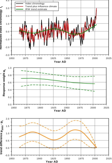
The first case from Table 2, that of Larch, detrended by RCS, is given in Fig. 3. The trend estimate (green line, up-per panel) shows non-stationary behavior at the record’s end, from 1970–2003. The lower panel shows that the trend esti-mate in the final year (µ2003)is significant larger than those for 1864–1917 and 1937–1995 (2-σ confidence limits). The response weightαˆt has a slightly decreasing pattern, which the LR test showed to be non-significant.
4 Discussion
We discuss two topics in this section: (i) the omission of data (truncation) over the final decades of a chronology, one method which has been used to deal with divergence-type phenomena; and (ii) potential implications of SRFs for screening procedures of proxy data.
4.1 Omission of data over recent decades
23 1
Fig. 1. SRF estimates for the MXD chronology derived at Coppermine. Period: 1933-2003. The
2
black line in the upper panel represents the normalized indices, the green line the estimated IRW trend 3
and the red line the trend plus influence of July-August temperatures. The response αˆ appears to be 4
time varying (middle panel, with 95% confidence limits). The trend differences with 95% confidence 5
limits are shown in the lower panel. 6
1930 1940 1950 1960 1970 1980 1990 2000 2010 Year AD -3.0 -2.0 -1.0 0.0 1.0 2.0
3.0 Index chronology
trend plus influence tem peratures IR W trend estim ate
N o rm a li z e d i n d e x c h ro n o lo g y It
1930 1940 1950 1960 1970 1980 1990 2000 2010
Year AD -0.5 0.0 0.5 1.0 1.5 R e s p o n s e w e ig h
t αααα
1930 1940 1950 1960 1970 1980 1990 2000 2010 Year AD -1.0 0.0 1.0 2.0 T re n d d if fe re n c e
µµµµ20
0
3
-µµµµt
Fig. 1. SRF estimates for the MXD chronology derived at Cop-permine. Period: 1933–2003. The black line in the upper panel represents the normalized indices, the green line the estimated IRW trend and the red line the trend plus influence of July-August tem-peratures. The responseαˆappears to be time varying (middle panel, with 95% confidence limits). The trend differences with 95% con-fidence limits are shown in the lower panel.
proxy might still be used for reconstruction purposes (e.g., Briffa et al., 2001; Cook et al., 2004; Wilson and Elling, 2004; Mann et al., 2008, SI). Esper et al. (2010) performed a sensitivity study in which the role of the calibration pe-riod was explicitly taken into account (amongst other factors such as standardization technique and instrumental data cor-rections). However, their study deviates from our approach herein in that no regression technique was applied.
One potential application of the SRF method in this con-text is that we can accurately follow the patterns ofαˆi,t and
ˆ
µt to determine if it might be advantageous to confine the response analysis to a shorter calibration period. As an illustration, we re-estimated the MXD series for Copper-mine, shown in Fig. 1, choosing the shorter calibration pe-riod 1933–1990. The results reveal a more variable response weight than shown in the middle panel of Fig. 1. Thus,
24 1
Fig. 2. SRF estimates for the Thelon TRW chronology. Period: 1950-2002. The black line represents
2
the normalized indices, the green line the estimated IRW trend and the red line the trend plus influence 3
of July-August temperatures. The IRW trend appears to be a straight line with statistical significant 4
differences for any trend difference [µt - µs]. The response αˆ appears to be constant: 0.47 ± 0.22.
5
6
1950 1960 1970 1980 1990 2000 2010
Year AD -3.0 -2.0 -1.0 0.0 1.0 2.0
3.0 Index chronology
IRW trend plus influence JA temperatures IRW trend estimate
In d e x c h ro n o lo g y It
Fig. 2. SRF estimates for the Thelon TRW chronology. Period: 1950–2002. The black line represents the normalized indices, the green line the estimated IRW trend and the red line the trend plus influence of July–August temperatures. The IRW trend appears to be a straight line with statistical significant differences for any trend difference [µt−µs]. The responseαˆ appears to be constant: 0.47±0.22.
the omission of recent data does not improve the stability of the climate-tree growth model in this case. We also re-estimated the larch example shown in Fig. 3. Theαˆtandµˆt patterns suggest that a re-estimation over the period 1864– 1950 yield values that are in fact stable. The estimation re-sults are shown in Fig. 4. There appears to be a small lin-ear trend, which is statistically non-significant. The response weight appears to be constant:αˆ=0.70±0.15. Therefore, this re-analysis shows that the RCS-detrended larch chronology shows a stable response over a shorter calibration period.
Taken together, the truncation of calibration periods seems to be a good means of retaining proxies which would not oth-erwise pass a screening procedure. However, one could ar-gue that if a loss of proxy-target sensitivity occurs in recent decades, it could also have occurred in the past. A notable example is during the MWP, when temperatures have been reconstructed for some regions to be comparable to those of the 20th century (Jones et al., 2009). This argument is in line with the Uniformitarian principle as formulated in the Introduction. The principle implies that the same kinds of limiting conditions affected the same kinds of processes in the same ways in the past as in the present; only the fre-quencies, intensities, and localities of the limiting conditions affecting growth may have changed (Fritts, 1976). Loehle (2009, p. 241) comes to a similar conclusion, using a math-ematical approach: “if a reconstruction already shows diver-gence, it is an indication that recent temperature are already in the non-linear zone; such reconstructions should not be used for evaluating past climates.”
25 1
Fig. 3. SRF estimates for Larch, standardized by RCS (first chronology in Table 2). Period:
1864-2
2003. The upper graph shows the index chronology (black line), the IRW trend (green line) and the 3
trend plus climate influence (red line). The middle panel shows time-varying response αˆt and the 4
lower panel the trend differences [µˆ2003 - µˆt]. The dashed lines represent 95% confidence limits.
5
1850 1875 1900 1925 1950 1975 2000 2025
Year AD -3.0 -2.0 -1.0 0.0 1.0 2.0 3.0 4.0 Index chronology Trend plus influence clim ate IRW trend estim ate
N o rm a li z e d i n d e x c h ro n o lo g y It
1850 1875 1900 1925 1950 1975 2000 2025
Year AD -0.5 0.0 0.5 1.0 1.5 2.0 tr e n d d if fe re n c e
µµµµ20
0
3
µµµµt
1850 1875 1900 1925 1950 1975 2000 2025
Year AD 0.0 0.2 0.4 0.6 0.8 1.0 R e s p o n s e ααααt R e s p o n s e w e ig h
t αααα
t
Fig. 3. SRF estimates for Larch, standardized by RCS (first chronol-ogy in Table 2). Period: 1864–2003. The upper graph shows the index chronology (black line), the IRW trend (green line) and the trend plus climate influence (red line). The middle panel shows time-varying responseαtˆ and the lower panel the trend differences [µˆ2003− ˆµt]. The dashed lines represent 95% confidence limits.
(air pollution, soil acidification, etc.), we could truncate the calibration period. However, this introduces a new prob-lem: how could we uniquely attribute instabilities to such (anthropogenic) drivers? E.g., in case of the example shown in Figs. 3 and 4 we do not have such a unique clue.
In conclusion, we feel that the omission of data over recent decades is not a sufficient means to accept a specific chronol-ogy for use in a reconstruction network.
4.2 SRFs and screening of proxy data
Since SRFs can potentially be used to detect pattern (in)stabilities, along with statistical significance testing, it is interesting to re-evaluate the two examples from the pre-ceding Section. Certainly, any two calibration/validation ap-proaches can show different results for specific proxies. For instance, one may split a calibration period into two parts of equal size and calculate correlation coefficients between the
26 1
Fig. 4 Larch data, standardized by RCS, 1864-1950. In this example we re-estimated the results
2
shown in Fig. 3. The response weight appears to be constant: αˆ = 0.70 ± 0.15. The explained variance 3
is 55%. The slightly increasing linear trend is statistically non-significant. 4
5
1850 1875 1900 1925 1950 1975 2000 2025
Year AD -3.0 -2.0 -1.0 0.0 1.0 2.0 3.0 4.0 Index chronology Trend plus influence climate IRW trend estimate
N o rm a li z e d i n d e x c h ro n o lo g y It
Fig. 4. Larch data, standardized by RCS, 1864–1950. In this ex-ample we re-estimated the results shown in Fig. 3. The response weight appears to be constant: αˆ=0.70±0.15. The explained vari-ance is 55%. The slightly increasing linear trend is statistically non-significant.
proxy and target variable over both periods. Supposing that bothR2values are considered reasonably strong, say above 0.44 (as in Table 1 of B¨untgen et al., 2009, for larch and splines) one might conclude that the results are satisfactory. In another approach, CE/RE values are calculated over the same two periods. Negative CE values might cause one to reject the proxy. This marked difference is explained from the fact that well-fitting models, leading to highR2values, might have a poor prediction performance on independent data (cf. National Research Council, 2006 – Fig. 9-3). This methodological uncertainty is real since both methods (us-ingR2values alone versus RE/CE values) can be found side by side in the recent reconstruction literature. The articles of D’Arrigo et al. and B¨untgen et al., mentioned above, together constitute only two such examples. Thus, how do the results from D’Arrigo et al. (R2 approach) and those of B¨untgen et al. (R2/RE/CE approach) relate to the results presented in Tables 1 and 2?
71 years for Coppermine). Third, non-homogeneities in the instrumental data may play a role, despite the GHCN tests. Therefore, we come to the same conclusion as D’Arrigo et al. (2009) that some of these series have potential losses in sensitivity to climate.
B¨untgen et al. split the calibration period in two and cal-culatedR2values as well as RE and CE values for each of the four chronologies (two standardization techniques and two tree species). They find CE values around zero for both spline-standardized series, a finding which is consis-tent with the findings presented herein in Table 2. Thus, the spline detrended series do not perform well in either ap-proach. For the RCS standardized series, much better CE val-ues are found, between 0.25 and 0.29, guaranteeing predic-tion skill. Squared correlapredic-tion coefficients over sub-periods vary between 0.18 and 0.55. B¨untgen et al. conclude that there is no indication of a DP for either species after scal-ing the RCS chronologies, although larch generally tracks summer temperature better than spruce (lowerR2 values). Our findings here show time-varying behavior for the RCS chronologies as well. After shortening the calibration pe-riod (data after 1950 omitted) we find stable responses for the RCS-standardized larch chronology. Unfortunately, this shortening does not guarantee stability in the past, as dis-cussed in Sect. 4.1.
Clearly, these two examples, covering three screening techniques, are not sufficient for a full evaluation of meth-ods. Further, any comparison of any three approaches will reveal results which differ in some detail. With that respect the analysis shown here is certainly incomplete and more re-search is needed.
5 Conclusions
Peer-reviewed literature has described unstable relationships between tree-ring proxies and climate target variables for re-cent decades at some northern and higher elevation sites, of-ten denoted by the term “divergence”. Within this context we have drawn attention to a statistical approach which is ideally suited for tracing instabilities in proxy-target cali-bration, that of stochastic response functions. This method is also well suited for performing proxy data screening prior to network aggregation. Our inferences in this study have mainly focused on methods of calibration and screen-ing within the field of dendroclimatology. However, the proposed technique is potentially applicable to the calibra-tion of other proxies besides tree rings. Furthermore, the (non-)equivalence of independent reconstructions can be ex-plored as shown by Wilson et al. (2010).
We draw the following conclusions:
1. Stochastic response functions are useful for providing insight when instabilities are expected to occur in gen-eration of climatic reconstructions. Changes in response and trend can be readily observed from year to year.
No specific time window is needed, in contrast with the MRF or moving correlations approach. Furthermore, the use of the Kalman filter allows us to test for time-dependent changes. It should be noted that the time sta-bility of the intercept and response weights are of equal importance (in the literature the (in)stability of the first term is never mentioned explicitly).
2. It is advisable to define a climate envelope and deter-mine whether hindcasts fall outside this envelope over the length of the climatic reconstruction. Tests for lin-earity are also important.
3. Stochastic response functions are ideally suited to lo-calize instabilities over time. However, if these instabil-ities occur in recent decades (“divergence”) and if the cause of these instabilities can not be traced/attributed to drivers which are only in operation during these re-cent decades, the omission of rere-cent decades in the cali-bration period is not a valid means of generating an un-biased reconstruction network.
4. Two examples have been discussed as illustrations of the potential application of stochastic response func-tions to climatic reconstrucfunc-tions. For both examples, we find screening results that are only partly comparable to those found using other methods of validation (R2, RE, CE). It is unclear if the stochastic response methodol-ogy would filter out more proxies than these traditional methods. Clearly, much more analysis is necessary to evaluate the various screening methods.
5. Given the policy relevance of paleoclimatic reconstruc-tions, dendrochronologists are especially advised to be more explicit about dealing with uncertainty in proxy screening.
Appendix A
Response function models in detail
Calibration of a tree growth/climate model is typically based on a linear regression relationship between a proxy It and some climate variable(s)Xt:
It=µ+α·Xt+εt (A1)
The suitability of model (A1) is typically tested by split-ting the calibration period in two or three sub-periods of gen-erally equal length. Model (A1) is then calibrated for one sub-period and used to estimate It values over the other sub-period(s). Finally, model performance is assessed using sev-eral statistics typically used in dendroclimatology: R, RE, CE and DW. Here, R stands for the well-known correlation coefficient. RE stands for the Reduction of Error statistic and is a measure for the prediction performance for the cali-bration period chosen. CE stands for the Coefficient of Effi-ciency statistic and measures the prediction performance for a particular validation period. For this reason the CE statistic is more stringent than the RE statistic. Please refer to Na-tional Research Council (2006, p. 92–95 for strengths and weaknesses of these statistics). DW stands for the Durbin Watson test, which tests for lag-1 autocorrelation in resid-uals of the calibration model. See Fritts (1976), Cook and Kairiukstis (1990), Cook et al. (1994) and National Research Council (2006) for details. B¨urger and Cubasch (2007) use the RE and CE statistics in combination with resampling schemes.
Stochastic response functions can be modeled by choosing a sub-model from the class of structural time series models (STMs), in combination with the discrete Kalman filter (Har-vey, 1989; Visser and Molenaar, 1995; Durbin and Koopman, 2001). These models allow the estimation of a regression model with time-varying coefficients:
It=µt+α1,t·X1,t+α2,t·X2,t+...+αm,t·Xm,t+εt (A2a) Here,It stands for a climate proxy, such as a standardized ring-width chronology, or the logarithm thereof (depend-ing on the additivity resp. multiplicativity assumptions in the growth model). The variablesXi,t may stand for stan-dardized climate variables or PCs thereof. The coefficients
α1,t, ...,αm,ttogether form the stochastic response function andεt is a white noise process with variance σε2. A time-dependent response is gained by defining m random walk models: αi,t=ai,t−1+ηi,t ,i=1, ...., m. Here, ηi,t stands for a noise process with zero mean and varianceση,i2 . These variances may be found by applying maximum likelihood optimization. For the trend componentµt, resembling the age-related trend plus external factors, the integrated ran-dom walk trend model (IRW model) is taken (Visser, 2004). This model reads asµt−2·µt+µt=ηm+1,t , withηm+1,t a white noise process with varianceση,m2 +1. Dendroclimatic consequences for chronology building and the selection of variables in the context of time-varying coefficients are de-scribed in Visser and Molenaar (1988), and van den Brakel and Visser (1996).
The discrete Kalman filter is an optimal filter in that it yields the minimum mean square error estimates (MMSE) forµtandαtalong with maximum likelihood estimation for unknown noise variances. This result holds if all noise pro-cesses are normally distributed. If noise propro-cesses involved do not follow a normal distribution, the Kalman filter still
yields the minimum mean square linear estimators (MM-SLE) forµtandαt. For details please refer to Harvey (1989, p. 111). All estimates shown in this article are based on smoothed estimates using a fixed-interval smoother.
As for initial values of noise variances we have chosen the approach of a so-called diffuse or non-informative prior. This means that we set the initial covariance matrix to the unity matrix with large numbers on the main diagonal. Thus, we simply “tell” the filter that we have no information what-soever at the first iteration. See Harvey (1989, p. 121) for de-tails. The consequence of this approach is that the filter needs some iterations to arrive at stable state-space estimates. For the models presented in Tables 1 and 2 of this article we have chosen for a transient period of 20 years. The consequence of a “diffuse prior” is that the innovations series starts after these 20 years. In the process of ML optimization the tran-sient period is excluded. See Harvey (1989, p. 256) for de-tails. We note that this transient period is not seen in Figs. 1 through 4. The reason is simply that these graphs do not show the filtered estimates forµt andαt, but the smoothed estimates.
The IRW trend model reduces to the well-known OLS fit of a straight line ifση,m2 +1 is set to zero. And constant re-sponses are found if the variancesση,i2 are set to zero. Thus, if all noise variances in model (A2a) are set to zero, this model reduces to
It=α0+β·t+α1·X1,t+α2·X2,t+...+αm·Xm,t+εt (A2b) For stationary data the term β will be zero and Eq. (A2b) equals the well-known multiple regression model.
The SRF model has similarities to the moving response functions (MRFs) (Biondi and Waikul, 2004) if the trend component is set to a random walk, rather than the IRW trend model. However, the advantage of SRFs over MRFs is that no window has to be chosen and, thus, that estimates are found for the full sample period. Furthermore, within the framework of SRFs the selection of variables can be per-formed over the whole calibration period (Visser and Mole-naar, 1988), while MRFs have to do that for a much shorter window, in the order of 50 years of length. This selection of variables may become problematic if the number of explana-tory variables becomes large (>24).
Acknowledgements. UB was supported by the EC project Millen-nium (grant 017008) and the SNSF project NCCR (grant Extract). We thank the CP reviewers for their thorough comments.
Edited by: C. Hatt´e
References
Ammann, C. M., Genton, M. G., and Li, B.: Technical Note: Cor-recting for signal attenuation from noisy proxy data in climate reconstructions, Clim. Past, 6, 273–279, doi:10.5194/cp-6-273-2010, 2010.
Auer, I., B¨ohm, R., Jurkovic, A., et al.: HISTALP – historical instru-mental climatological surface time series of the Greater Alpine Region, Int. J. Climatol., 27, 17–46, 2007.
Biondi, F. and Waikul, K.: DENDROCLIM2002: a C++ program for statistical calibration of climate signals in tree-ring chronolo-gies, Comput. Geosci., 30, 303–311, 2004.
Blasing, T. J., Solomon, A. M., and Duvick, D. N.: Response func-tions revisited, Tree-ring Bulletin, 44, 1–15, 1984.
Briffa, K. R., Osborn, T. J., Schweingruber, F. H., Harris, I. C., Jones, P. D., Shiyatov, S. G., and Vaganov, E. A.: Low-frequency temperature variations from a northern tree ring density network, J. Geophys. Res., 106, 2929–2941, 2001.
B¨untgen, U., Frank, D. C., Schmidhalter, M., Neuwirth, B., Seifert, M., and Esper, J.: Growth/climate response shift in a long sub-alpine spruce chronology, Trees Structure and Function, 20, 99– 110, 2006.
B¨untgen, U., Frank, D., Wilson, R., Carrer, M., Urbinati, C., and Esper, J.: Testing for tree-ring divergence in the European Alps, Global Change Biology, 14, 2443–2453, 2008.
B¨untgen, U., Wilson, R., Wilmking, M., Niedzwiedz, T., and Br¨auning, A.: The ‘Divergence Problem’ in tree-ring research, Trace, 7, 212–219, 2009.
B¨urger, G.: On the verification of climate reconstructions, Clim. Past, 3, 397–409, doi:10.5194/cp-3-397-2007, 2007.
Carrer, M. and Urbinati, C.: Assessing climate-growth relation-ships: a comparative study between linear and non-linear meth-ods, Dendrochronologia, 19, 2443–2453, 2001.
Carrer, M., Nola, P., Eduard, J. L., Motta, R., and Urbinati, C.: Re-gional variability of climate-growth relationships in Pinus cem-bra high elevation forests in the Alps, J. Ecol., 95, 1072–1083, 2007.
Cook, E. R. and Kairiukstis, L. A. (Eds.): Methods of dendroclima-tology. Kluwer Academic Publishers, Dordrecht, 1990. Cook, E. R., Briffa, K. R., and Jones, P. D.: Spatial regression
meth-ods in dendroclimatology: a review and comparison of two tech-niques, Int. J. Climatol., 14, 379–402, 1994.
Cook, E. R. and D’Arrigo, R. D.: A well-verified, multiproxy re-construction of the winter north atlantic oscillation index since A.D. 1400, J. Climate, 15, 1754–1764, 2002.
Cook, E. R., Esper, J., and D’Arrigo, R.: Extra-tropical North-ern Hemisphere land temperature variability over the past 1000 years, Quat. Sci. Rev., 23, 2063–2074, 2004.
D’Arrigo, R. D., Kaufmann, R. K., Davi, N., Jacoby, G. C., Laskowski, C., Myneni, R. B., and Cherubini, P.: Thresholds for warming-induced growth decline at elevational tree line in the Yukon Territory, Canada, Global Biogeochem. Cycles, 18, GB3021, doi:10.1029/2004GB002249, 2004.
D’Arrigo, R. D., Wilson, R., Liepert, B., and Cherubini, P.: On the ‘divergence problem’ in Northern forests. A review of the tree-ring evidence and possible causes, Global Planet. Change, 60(3–4), 289–305, 2008.
D’Arrigo, R. D., Jacoby, G., Buckley, B., Sakulich, J., Frank, D., Wilson, R., Curtis, A., and Anchukaitis, K.: Tree growth and in-ferred temperature variability at the North American Arctic tree-line, Global Planet. Change, 65, 71–82, 2009.
De Jong, P. and Mackinnon, M. J.: Covariances for smoothed esti-mates in state space models, Biometrika, 75(3), 601–602, 1988. Dobrovoln´y, P., Moberg, A., Br´azdil, R., Pfister, C., Glaser, R.,
Wil-son, R., van Engelen, A., Liman´owka, D., Kiss, A., Haliˇckov´a, M., Mackov´a, J., Riemann, D., Luterbacher, J., and B¨ohm, R.: Monthly, seasonal and annual temperature reconstructions for Central Europe derived from documentary evidence and instru-mental records since AD 1500, Climatic Change, online version, 2010.
Durbin, J. and Koopman, S. J.: Time series analysis by state space methods, Oxford Statistical Science Series, 24, 253 pp, 2001. Esper, J., Cook, E. R., and Schweingruber, F. H.: Low-frequency
signals in long tree-ring chronologies for reconstructing past temperature variability, Science, 295(5563), 2250–2253, 2002. Esper, J. and Frank, D.: Divergence pitfalls in tree-ring research,
Climatic Change, 94, 261–266, 2009.
Esper, J., Frank, D., B¨untgen, U., Verstege, A., Hantemirov, R. M., and Kirdyanov, V.: Trends and uncertainties in Siberian indica-tors of 20th century warming, Global Change Biol., 16, 386–398, 2010.
Fritts, H. C.: Tree rings and climate, Academic Press, London, 567 pp, 1976.
Harvey, A. C.: Forecasting, structural time series models and the Kalman filter, Cambridge University Press, 554 pp, 1989. Hegerl, C. G., Crowley, T. J., Allen, M., Hyde, W. T., Pollack, H. N.,
Smerdon, J., and Zorita, E.: Detection of human influence on a new, validated 1500-year temperature reconstruction, J. Climate, 20, 650–666, 2007.
Hughes, M. K.: Dendrochronology in climatology – the state of the art, Dendrochronologia, 20(1–2), 95–116, 2002.
Jansen, E., Overpeck, J., Briffa, K. R., Duplessy, J.-C., Joos, F., Masson-Delmotte, V., Olago, D., Otto-Bliesner, B., Peltier, W. R., Rahmstorf, S., Ramesh, R., Raynaud, D., Rind, D., Solom-ina, O., Villalba, R., and Zhang, D.: Palaeoclimate, in: Climate Change 2007, edited by: Solomon, S., Qin, D., Manning, M., et al., The Physical Science Basis, Cambridge University Press, UK, 2007.
Jones, P. D., Briffa, K. R., Osborn, T. J., et al.: High-resolution palaeoclimatology of the last millennium; a review of current status and future prospects, The Holocene, 19, 3–49, 2009. Loehle, C.: A mathematical analysis of the divergence problem in
dendroclimatology, Climatic Change, 94, 233–245, 2009. Mann, M. E., Zhang, Z., Hughes, M. K., Bradley, R. S., Miller, S.
K., Rutherford, S., and Ni, F.: Proxy-based reconstructions of hemispheric and global surface temperature variations over the past two millennia, PNAS, 105(36), 13252–13257, 2008. National Research Council: Surface temperature reconstructions
for the last 2,000 years, The National Academies Press, Wash-ington D.C., 145 pp, 2006.
at Mt. Patscherkofel (Tyrol, Austria) since the mid-1980s, Trees, 22, 31–40, 2008.
Oppo, D. W., Rosenthal, Y., and Linsley, B. K.: 2,000-year-long temperature and hydrology reconstructions from the Indo-Pacific warm pool, Nature, 460, 1113–1116, 2009.
Pisaric, M. F. J., Carey, S. K., Kokelj, S. J., and Youngblut,
D.: Anomalous 20t h century tree growth, Mackenzie Delta,
Northwest Territories, Canada, Geophys. Res. Lett., 34, L05714, doi:10.1029/2006GL029139, 2007.
Rozas, V.: Dendrochronology of pedunculate oak (Quercus robur L.) in an old-growth pollarded woodland in northern Spain: tree-ring growth responses to climate, Ann. For. Sci., 62, 209–218, 2005.
Schiermeier, Q.: The real holes in climate science, Nature, 463, 284–287, 2010.
Van den Brakel, J. and Visser, H.: The influence of environmen-tal conditions on tree-ring series of Norway spruce for different canopy and vitality classes, Forest Sci., 42(2), 206–219, 1996. Van Deusen, P.: Evaluating time-dependent tree ring and climate
relationships, J. Environ. Qual., 19, 481–488, 1990.
Visser, H.: Analysis of tree ring data using the Kalman filter tech-nique, IAWA Bulletin n.s., 7(4), 289–297, 1986.
Visser, H.: Estimation and detection of flexible trends, Atmos. En-viron., 38, 4135–4145, 2004.
Visser, H. and Molenaar, J.: Kalman filter analysis in dendroclima-tology, Biometrics, 44, 929–940, 1988.
Visser, H. and Molenaar, J.: Estimating trends and stochastic re-sponse function in dendroecology with an application to fir de-cline, Forest Sci., 38(2), 221–234, 1992.
Visser, H. and Molenaar, J.: Trend estimation and regression analy-sis in climatological time series: an application of structural time series models and the Kalman filter, J. Climate, 8(5), 969–979, 1995.
Visser, H. and Petersen, A. C.: The likelihood of holding outdoor skating marathons in the Netherlands as a policy-relevant indica-tor of climate change, Clim. Change, 93, 39–54, 2009.
Wilmking, M., Juday, G. P., Barber, V. A., and Zald, H. S. J.: Recent climate warming forces contrasting growth responses of white spruce at treeline in Alaska through temperature thresh-olds, Global Change Biology, 10, 1724–1736, 2004.
Wilmking, M., D’Arrigo, R. D., Jacoby, G., and Juday, G.: Diver-gent growth responses in circumpolar boreal forests, Geophys. Res. Lett., 32, L15715, doi:10.1029/2005GL023331, 2005. Wilmking, M. and Myers-Smith, I.: Changing climate sensitivity
of black spruce (Picea Mariana Mill.) in a peatforest land-scape in Interior Alaska, Dendrochronologia, 25, 167–175, 2008. Wilmking, M. and Singh, J.: Eliminating the “divergence problem” at Alaska’s northern treeline, Clim. Past Discuss., 4, 741–759, doi:10.5194/cpd-4-741-2008, 2008.
Wilson, R. and Elling, W.: Temporal instability in
tree-growth/climate response in the lower Bavarian forest region: im-plications for dendroclimatic reconstruction, Trees, 18, 19–28, 2004.
Wilson, R., D’Arrigo, R. D., Buckley, B., B¨untgen, U., Esper, J., Frank, D., Luckman, B., Payette, S., Vose, R., and Young-blut, D.: A matter of divergence: tracking recent warming at hemispheric scales using tree ring data, J. Geophys. Res., 112, D17103, doi:10.1029/2006Jd008318, 2007.
Wilson, R., Cook, E. R., D’Arrigo, R. D., Riedwyl, N., Evans, M. N., Tudhope, A., and Allan, R.: Reconstructing ENSO: the influ-ence of method, proxy data, climate forcing and teleconnections, J. Quat. Sci., 25(1), 62–78, 2010.
Woodhouse, C. A.: Artificial neural networks and dendroclimatic reconstructions: an example from the Front Range, Colorado, USA, Holocene, 9, 521–529, 1999.