www.atmos-meas-tech.net/9/2947/2016/ doi:10.5194/amt-9-2947-2016
© Author(s) 2016. CC Attribution 3.0 License.
An empirical method to correct for temperature-dependent
variations in the overlap function of CHM15k ceilometers
Maxime Hervo1, Yann Poltera1,a, and Alexander Haefele1 1MeteoSwiss, Payerne, Switzerland
anow at: Institute for Atmospheric and Climate Science, ETH, Zurich, Switzerland
Correspondence to:Maxime Hervo ([email protected])
Received: 29 January 2016 – Published in Atmos. Meas. Tech. Discuss.: 18 February 2016 Revised: 31 May 2016 – Accepted: 15 June 2016 – Published: 12 July 2016
Abstract.Imperfections in a lidar’s overlap function lead to artefacts in the background, range and overlap-corrected li-dar signals. These artefacts can erroneously be interpreted as an aerosol gradient or, in extreme cases, as a cloud base leading to false cloud detection. A correct specification of the overlap function is hence crucial in the use of automatic elastic lidars (ceilometers) for the detection of the planetary boundary layer or of low cloud.
In this study, an algorithm is presented to correct such arte-facts. It is based on the assumption of a homogeneous bound-ary layer and a correct specification of the overlap function down to a minimum range, which must be situated within the boundary layer. The strength of the algorithm lies in a sophisticated quality-check scheme which allows the reli-able identification of favourreli-able atmospheric conditions. The algorithm was applied to 2 years of data from a CHM15k ceilometer from the company Lufft. Backscatter signals cor-rected for background, range and overlap were compared us-ing the overlap function provided by the manufacturer and the one corrected with the presented algorithm. Differences between corrected and uncorrected signals reached up to 45 % in the first 300 m above ground.
The amplitude of the correction turned out to be tempera-ture dependent and was larger for higher temperatempera-tures. A lin-ear model of the correction as a function of the instrument’s internal temperature was derived from the experimental data. Case studies and a statistical analysis of the strongest gradi-ent derived from corrected signals reveal that the temperature model is capable of a high-quality correction of overlap arte-facts, in particular those due to diurnal variations. The pre-sented correction method has the potential to significantly improve the detection of the boundary layer with
gradient-based methods because it removes false candidates and hence simplifies the attribution of the detected gradients to the plan-etary boundary layer. A particularly significant benefit can be expected for the detection of shallow stable layers typical of night-time situations.
The algorithm is completely automatic and does not re-quire any on-site intervention but rere-quires the definition of an adequate instrument-specific configuration. It is therefore suited for use in large ceilometer networks.
1 Introduction
Due to technological advances in recent decades, state-of-the-art ceilometers can nowadays be considered automatic elastic lidars. They are increasingly used for profiling of aerosols, including the detection of volcanic particles (e.g. Emeis et al., 2011; Flentje et al., 2010; Wiegner et al., 2012) and the determination of the planetary boundary layer (Ha-effelin et al., 2012). As for all lidars, there is a zone close to the ground where the telescope field of view does not fully overlap with the laser beam and where geometric and instru-mental effects therefore distort the measured backscatter pro-file. This effect is accounted for with the so-called overlap function, which describes the signal loss due to the overlap effect as a function of altitude. A correct determination of the overlap function is crucial for aerosol profiling in the zone of partial overlap, i.e. in the boundary layer.
ef-fects, the precision of such models is generally not sufficient. For example the energy distribution of the laser beam can be ambiguous (Sasano et al., 1979), the transmittance of inter-ference filters may depend on the incident angle (Sasano et al., 1979) or the laser beam might not be well focused on the receiver and will thus alter the measured power (Roberts and Gimmestad, 2002). One of the main issues is the impact of temperature on the optical components (Campbell et al., 2002; Welton and Campbell, 2002).
To determine the overlap function experimentally, several approaches are possible, such as observing a homogeneous atmosphere (Sasano et al., 1979; Welton et al., 2000), us-ing a Raman signal (Wandus-inger and Ansmann, 2002) or hard target (Vande Hey et al., 2011) or using a reference instru-ment with a known overlap function (Guerrero-Rascado et al., 2010; Reichardt et al., 2012). Most of these methods re-quire rather costly installations or human intervention and are thus not suited to larger networks of automatic lidars.
The only method that can potentially be applied to a large network at no additional cost is, in our opinion, the use of a vertically homogeneous atmosphere (constant aerosol backscatter and aerosol extinction coefficients). To identify cases with a homogeneous atmosphere, Sasano et al. (1979) proposed to use the ratio between the received power from two altitudes and require that it is stable over time. Since the assumption of a homogeneous atmosphere is not justified across the interface between the boundary layer and the free troposphere, this method is only suited to instruments that reach full overlap within a few hundred metres, i.e. within the boundary layer (Sasano et al., 1979) or for instruments with a correctly specified overlap down to a minimum range within the boundary layer (in this work).
Welton et al. (2000) proposed to perform horizontal mea-surements such that the assumption of a homogeneous atmo-sphere also holds for instruments which reach full overlap only after a few thousand metres. Methods using horizontal or inclined measurements are the most common, both in the scientific community and by manufacturers (Campbell et al., 2002; Biavati et al., 2011). However, these methods assume that the overlap function does not change between vertical and inclined alignment of the system, an assumption which may not be justified for certain instruments. Furthermore, the inclination of instruments requires important mechanical de-velopments or human intervention.
Since instrumental parameters are not perfectly constant in time, the overlap function needs to be re-evaluated at reg-ular intervals. Hence, for dense networks of lidars, an au-tomatic approach which requires minimal system modifica-tions is needed. In this study, we propose an extension of the method by Sasano et al. (1979), combined with the assump-tion that a first guess of the overlap funcassump-tion is available. We will show that this method can be implemented for existing instruments without on-site intervention and that it is suited to large networks of automatic lidars. The algorithm as
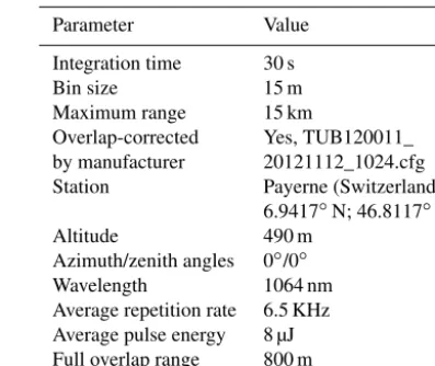
pre-Table 1.Instrument parameters.
Parameter Value
Integration time 30 s
Bin size 15 m
Maximum range 15 km
Overlap-corrected Yes, TUB120011_ by manufacturer 20121112_1024.cfg
Station Payerne (Switzerland,
6.9417◦N; 46.8117◦E)
Altitude 490 m
Azimuth/zenith angles 0◦/0◦
Wavelength 1064 nm
Average repetition rate 6.5 KHz Average pulse energy 8 µJ Full overlap range 800 m
sented here is optimized for the CHM15k ceilometer but can in principle be adapted to other instruments.
The paper is organized as follows: the instrument for which the method has been implemented and tested is de-scribed in Sect. 2, and in Sect. 3 a detailed description of the method is given. Results are presented in Sect. 4, and in Sect. 5 we discuss temperature effects on the overlap func-tion and propose a model to correct such effects. Examples of the performance of the correction for the determination of the boundary layer height are presented in Sect. 6, followed by a summary and conclusions.
2 The CHM15k-Nimbus ceilometer
The CHM15k-Nimbus ceilometer is a biaxial photon-counting lidar (1064 nm, 6.5 KHz, 8 µJ) manufactured by the company Lufft Mess- und Regeltechnik GmbH (previously manufactured by Jenoptik). The emitter and the receiver are placed next to each other in the optical module, with a centre-to-centre distance of 12 cm. More information about a simi-lar instrument can be found in Wiegner and Geiß (2012). For the instrument considered in this study, the lowest level of non-zero (full) overlap is at approximately 180 (800) m. Its relevant parameters are given in Table 1.
3 Method 3.1 Physical basis
The lidar equation relates received power per pulse,P, as a function of range,r, and time,t, to instrumental and atmo-spheric parameters as follows:
P (r, t )= (1)
1
r2CL(t )CCHM(t )O(r, t )β(r, t )e
−2Rr 0α(r
0
,t )dr0+B(t ).
CLis the time-dependent calibration factor, andCCHMis a factor accounting for variations in the sensitivity of the re-ceiver. CCHM is the product of the variables “p_calc” and “scaling” provided by the manufacturer.αandβare the ex-tinction and backscatter coefficient, respectively, andBis the background normalized by the number of laser pulses.O(rt )
is the range and time-dependent overlap function which can be expressed with a temporally constant overlap function provided by the manufacturer, OCHM(r), and a correction function,fc(r, t ), as follows:
O(r, t )=OCHM(r)/fc(r, t ). (2) The standard instrument output, βraw (variable “beta_raw” provided by the manufacturer), is the normalized and back-ground, range and overlap-corrected signal defined as
βraw(r, t )=
(P (r, t )−B(t ))r2 CCHM(t )OCHM(r)
. (3)
We define the corrected instrument output as
βcorrected(r, t )=βraw(r, t )fc(r, t ), (4) which is proportional to the attenuated backscatter coeffi-cient, defined as
βatt(r, t )=β(r, t )e−2 Rr
0α(r 0,t )dr0
. (5)
The factor of proportionality is the calibration factor, as can be shown using Eqs. (1) and (4). The algorithm to cal-culate the correction functionfc(r, t )is based on two main assumptions:
1. The aerosol extinction and backscatter coefficients are constant in a range interval [0, R]and during the time period of observation (assumption of homogeneous at-mosphere).
2. The overlap function is known with low uncertainty in the range interval[ROK,∞], withROK≤R.
Under these assumptions, the aerosol lidar ratio (also de-fined in the literature as extinction-to-backscatter ratio) is constant in the range [0, R]. The aerosol backscatter coef-ficient (βp)is therefore proportional to the aerosol extinc-tion coefficient (αp)in the considered range. The molecular
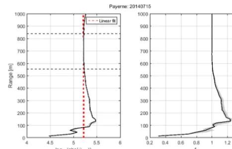
Figure 1.Left panel: logarithm of the absolute value of the range corrected signal measured at Payerne on 15 July 2014 from 00:25 to 01:20. The red line represents the linear fit performed between the two black dashed lines. Right panel: corresponding correction function.
backscatter and extinction coefficients, respectivelyβm and
αm, depend on atmospheric density and vary with range. In the range[0, R]Eqs. (1) to (3) can be written as follows, with time dependence neglected for clarity:
log(βraw(r))+log(fc(r))=log(CL)+log βp (6)
−2αpr+log
1+βm(r)
βp −2 r Z 0
αm(r0)dr0.
Using the aerosol lidar ratioLand a molecular lidar ratio equal to 8π3, Eq. (6) can be rewritten as follows:
log(βraw(r))+log(fc(r))=log(CL)+log
αp
L
(7)
−2αpr+log
1+3Lαm(r)
8π αp
| {z }
A1(r)
−2
r Z
0
αm(r0)Dr0
| {z }
A2(r)
.
For a standard atmosphere and at a wavelength of 1064 nm, assuming a lidar ratio between 20 and 120 sr and a particle extinction coefficient between 0 and 100 Mm−1, the 5th term (A2)is in the order of 0.01 % of the total signal.
A2is neglected for the rest of the calculations. Noting that the 4th term (A1)is close to straight line, the right hand side of Eq. (7) forms itself, in good approximation, into a straight line:
log(βraw(r))+log(fc(r))=A+Br∀r∈[0, R]. (8) Assuming further that OCHM(r) is correct in the range
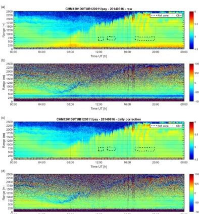
Figure 2.CHM15k measurements at Payerne for 16 June 2014.(a, c): Logarithm of the range corrected signal.(b, d): Gradient of the range corrected signal,(a)and(b): without correction and(c, d): with overlap correction. The reference zones from which the overlap correction was calculated are circled with black dashed lines.
The correction function in the range[0, R]is given by the difference between the fit (right hand side of Eq. 8) and the data as follows:
fc(r)=e−(log(βraw(r))−(A+Br))∀r∈ [0, R]. (9) An example of fitting Eq. (8) to real data is presented on Fig. 1, left panel. The corresponding correction functionfc is represented on the right panel.
3.2 Outline of the algorithm
While the approach presented in the previous section is quite straightforward, the implementation of an automatic algo-rithm is not. The most difficult parts are the selection of
favourable atmospheric conditions and the quality control of the result. These two aspects are discussed in detail in Ap-pendix A, while only a brief description of the algorithm is given below.
The algorithm processes a swath of 24 h of data, for which one overlap correction function is derived. The swath is split into 282 intervals of length1T =30 min with starting times
tievery 5 min from 00:00 to 23:30. For each time interval, the
homo-Figure 3.Overlap functions for 16 June 2014. The thick black line is the median overlap function for this day. The dashed line repre-sents the overlap function provided by the manufacturer.
Figure 4.Success rate of the algorithm for 2 years of data.
geneous. Whereas ROK is instrument specific and constant throughout the processing, RMAX has to be determined for each time interval (as described in Appendix A). A series of fits is performed in the fitting interval [ROKRMAX]from which each one undergoes a sequence of quality checks to evaluate the quality and the plausibility of the fit itself and the obtained overlap correction functions. The final overlap correction function for the entire swath is taken as the median of all overlap correction functions that pass the quality check. This median is hereafter referred to as the “daily correction”.
4 Results
4.1 Case study: 16 June 2014
An example of a successful correction of the overlap function is shown in Fig. 2. This day is representative of a typical plan-etary boundary layer development (Stull, 1988). The residual layer is visible at night as well as the convective layer that
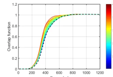
Figure 5.Overlap functions retrieved for Payerne ceilometer in 2013 and 2014. The colours represent the ceilometer internal tem-perature when the overlap functions were calculated.
developed during the day. An enhancement of the signal cen-tred at 250 m is visible all day (Fig. 2a). This feature becomes very pronounced when plotting the gradient of the range cor-rected signal (Fig. 2b) and must be attributed to artefacts in-duced by inaccuracies in the overlap function provided by the manufacturer.
The algorithm described in Sect. 3.2 was applied for this day. The areas marked with dashed lines indicate the time and height intervals, where Eq. (8) could be fit to the data. For this day, 144 overlap correction functions were selected by the al-gorithm for 44 out of the 282 time intervals of the swath (for details see Appendix A). The original and the corrected over-lap functions are shown in Fig. 3. The overover-lap function pro-vided by the manufacturer agrees well down to 600 m, which is simply a result of the fact that the function provided by the manufacturer is considered correct down to this altitude. Be-low, the original overlap function underestimates overlap by up to 45 % around 250 m (where the overlap value provided by the manufacturer is about 0.2).
The median of the corrected overlap functions was applied to the range corrected signal (Fig. 2c) and the gradient recal-culated (Fig. 2d). The example demonstrates nicely that the artefact disappears when the overlap correction is applied. 4.2 Long-term variability
Figure 6. Relative difference between corrected and uncorrected signal against internal temperature.
The obtained overlap functions (Fig. 5) show a large vari-ability and discrepancies up to 50 % with respect to the val-ues provided by the manufacturer. A seasonal cycle is present in the overlap correction with higher values in summer than in winter (not shown).
Assuming that this seasonal cycle is caused by variations in the temperature of the components, the daily overlap func-tions in Fig. 5 are displayed as a function of the median of the internal temperature measurements corresponding to the successful candidates (see Sect. 3.2 and Appendix A). Fig-ure 5 reveals a clear dependence of the overlap function on the internal temperature with higher values for warmer tem-peratures. It can further be seen that the overlap function pro-vided by the manufacturer corresponds to corrected overlap functions at low internal temperatures. This temperature de-pendence is further analysed in the following section and a model to correct for temperature effects is proposed.
5 Effect of the internal temperature
Fluctuations of the ambient temperature influence the tem-perature of the laser and the optical and electronic compo-nents. According to the manufacturer, the most temperature-dependent part of the system is the spatial sensitivity of the photodetector (H. Wille, personal communication, 2016). This in turn directly affects the overlap function.
The norm of the relative difference between corrected and uncorrected signal is represented as a function of the internal temperature (Fig. 6) and reveals a clear correlation. The dif-ference between the overlap function provided by the manu-facturer and the overlap function calculated by the algorithm increases with the temperature.
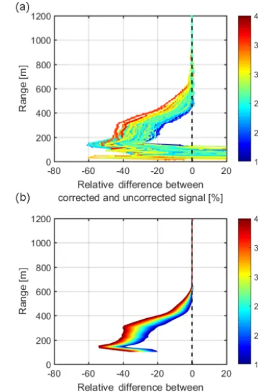
The impact of the temperature on the overlap function is now revealed and can be investigated further. Figure 7a shows the relative difference between the corrected and un-corrected signals at each altitude. The shape of the rela-tive difference is in agreement with the artefact described in Sect. 4.1. In this figure, the colour of each line is given by the temperature. The difference between corrected and un-corrected signal reached 45 % at a range of 250 m for 7 June
Figure 7.Relative difference between corrected and uncorrected signal. Upper panel: from measurements. Lower panel: with model. The colour represents the internal temperature of the instrument.
2014 when the median internal temperature was over 35◦C.
On the other hand, when the internal temperature was below 20◦C on 11 March 2014, the difference decreased to 20 %.
In the following, a simple model to correct this tempera-ture effect is described. At each range the relative difference between the corrected and uncorrected signals is assumed to depend linearly on the mean internal temperature. The coef-ficients for each range are determined by a linear fitting of the relative difference at this range (Fig. 7a). The resulting model is presented in Fig. 7b. To better highlight the temper-ature dependence in Figs. 5, 6 and 7a, 21 outliers have been identified and discarded (out of the 141 daily overlap func-tion correcfunc-tions). However to calculate the model coefficients used throughout the study, all data points were considered.
The performance of the model to correct artefacts is as-sessed in the next section. The major advantages of the model are the possibilities to correct for short-term variations on scales of hours (day/night) and to correct data in real time.
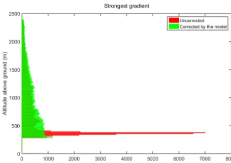
Figure 9.Histogram of the altitude of the strongest 5 min gradients calculated in 2013 and 2014. Uncorrected data are represented in red and data corrected with the temperature model in green.
range of internal temperatures that have to be expected for the site.
6 Effect of the overlap correction on edge detection In almost all boundary layer detection algorithms using aerosols as tracers, the detection of edges or gradients in the backscatter data is the first step. More or less sophisticated approaches are then chosen to attribute one of the detected edges or gradients to the planetary boundary layer height (PBL). This attribution is a very important step in the de-tection of the PBL but is beyond the scope of this study. This section is therefore limited to demonstrate the effect of our overlap correction method on the detection of aerosol gradi-ents. It is obvious that removing false candidates will also naturally improve the attribution procedure.
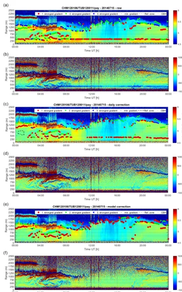
6.1 Case study: 15 July 2014
In Fig. 8, the performance of the temperature model is com-pared with corrections made with a single daily overlap func-tion (as in Sect. 4.1). Figure 8a, c and e show the logarithm of the range-corrected signal (calledSin Appendix A) mea-sured at Payerne on 15 July 2014. For this day an aerosol layer up to roughly 1500 m is clearly visible. Figure 8b, d and f show the corresponding gradient calculated together with the time series of the three strongest gradients as well as the lowest gradient. The gradients were calculated ev-ery 5 min from smoothed range corrected signals (below the cloud base height if any) and gradients of low magnitude were neglected.
If no correction is applied on CHM15k measurements, the strongest gradient is very often located at a constant altitude (Fig. 8a). By applying the algorithm described in the Ap-pendix, an overlap correction was determined using a
homo-geneous layer below 800 m from 00:30 to 01:30 (Figure 8c and d). Using this overlap correction significantly improved the detection of the strongest gradient at the top of the aerosol layer around 1100 m. For this day, the external temperature varied between 11 and 25◦C and the internal temperature between 22 and 30◦C. This change in temperature had an impact on the overlap function, meaning that the overlap correction retrieved around 01:00 does not perfectly correct the overlap artefact for the entire day. With the temperature model described in Sect. 5, the artefact can be almost per-fectly removed for the entire day (Fig. 8f). Consequently, false candidates attributable to the artefact, induced by inac-curacies in the overlap function, could be almost completely removed (Fig. 8e).
6.2 Long-term variability
The impact of the overlap correction on the detection of the strongest gradient was tested for the years 2013 and 2014. As in Sect. 6.1, gradients were calculated every 5 min, and the strongest at each time step was selected. The strongest gradient was chosen since this can be considered as a simple attribution solution to the boundary layer (Haeffelin et al., 2012). Figure 9 represents the frequency distribution of the height of this strongest gradient. Uncorrected data are shown in red and the results after the correction with the model in green. For the uncorrected data, a clear spike is visible around 360 m. This spike corresponds to the artefact induced by the uncorrected overlap function described previously. Af-ter the correction, this spike disappears and permits more gradient detections between 400 and 1000 m which are phys-ically meaningful. These gradients were previously masked by some erroneous gradient detections at the altitude of the spike (around 360 m).
The presented correction method thus has the potential to significantly improve the detection of the boundary layer us-ing gradient-based methods because it removes false candi-dates, e.g. in situations of well-mixed convective boundary layer, and hence simplifies the attribution of the detected gra-dients to the planetary boundary layer. A particularly high benefit can be expected for the detection of shallow stable layers typical in night-time situations.
7 Summary and conclusions
function. Here, a method has been presented to correct the overlap function, which is suited for automatic use in large networks, since it does not require any manipulation of the instrument. The method is based on the assumption that the atmosphere is homogeneous over a given time and range in-terval, in which the overlap function is known to have satis-factory quality. A polynomial of degree one is fit to the data in this interval and a correction function can be computed under the assumption that the atmosphere is also homoge-neous from the ground up to the lower boundary of the fitting range interval. The novelty of the method lies in the imple-mentation rather than in the approach itself, the latter being based on Sasano et al. (1979). A series of checks based on the spatio-temporal gradient is performed to identify homo-geneous conditions and the appropriate fitting interval. The obtained fits and the derived correction functions for a 24 h swath of data undergo thorough quality checking using a per-mutation scheme and stringent tests for the homogeneity of the corrected data.
Appendix A: Algorithm details
The different ranges (R...)and thresholds (κ...)used in the
following paragraphs are explained in Table A1. The values chosen for the implementation of a CHM15k lidar operated in the configuration are specified in Table 1. The algorithm processes a swath of 24 h of data for which one overlap cor-rection function is derived. First, the swath is split into 282 intervals of length1T =30 min, with starting timestievery
5 min from 00:00 to 23:30.
Determination of the fitting intervals
During this step, it is determined whether during the consid-ered time interval[ti, ti+1T], i∈1. . .282, there is a range
RMAX below which the atmospheric conditions satisfy the assumptions of homogeneity and thus where fitting intervals [R1, R2]∈ [ROKRMAX]can be constructed and tested.
Note that theRMAXvalue may change from one time inter-val to another and is limited byRMAX,MAX, usually inside the boundary layer.RMAX,MAX determines the maximum range below which homogeneous conditions can be expected. This parameter is not critical for the results but saves computa-tional time, as it restricts the total amount of fitting intervals which need to be tested.ROKdetermines the minimum range above which the manufacturer’s overlap function is believed to be accurate enough to allow the fitting procedure. TheROK andRMAX,MAXvalues depend on the instrument and site and are fixed for all calculations.
In order to calculateRMAX, the following series of checks are applied:
1. Data availability and bad weather: data availability must be 100 %; i.e. the time interval must consist here of 60 non-erroneous profiles, and within the time interval no precipitation or fog (bad weather) should occur, be-cause these events result in saturated, inhomogeneous signals. Weather information is taken here on a profile-by-profile basis directly from the ceilometer’s output (sky condition index), but it could also be taken from surface station measurements.
2. Cloud and signal-to-noise limitation: the fitting inter-val should not contain clouds (which result in peaks in the signal) and should not be too noisy. Therefore, the rangeRCLOUDof the lowest cloud base height dur-ing the whole time interval is identified, as well as the range of the lowest maximum detection height, RSNR. Cloud base heights and maximum detection heights are taken here on a profile-by-profile basis directly from the ceilometer’s output, but they could be calculated as well.
3. Test for homogeneity: here we check if characteristic properties of a homogeneous atmosphere are present. The 60 profiles of log10(abs(βraw))are considered. For
brevity, log10(abs(βraw))is hereafter referred to asS. At 1064 nm, because of the limited molecular influence, a homogenous atmosphere yields a profile ofSclose to a line. Therefore, almost vanishing spatial fluctuations of
Sare expected. These fluctuations can however only be checked starting from the rangeROKwhere the overlap function is known with satisfactory accuracy. Below this range artificial gradients may appear due to the incorrect manufacturer’s overlap correction. Temporal fluctua-tions inS, which should remain small, are checked from the ground up. The ground-levelRGROUNDis taken here as the lowest range where the overlap function is larger than 0.05. Below this range the signal is usually too noisy to be processed. The interval[ti, ti+1T]is split
into subintervals of duration1Ts=10 min starting ev-ery 30 s fromtiuntilti+1T−1Ts. All statistical
vari-ables and temporal gradients in the following are de-rived from these subintervals.
3.1 Temporal homogeneity:
3.1.1 For each range between RGROUND and
RMAX,MAX, the ratio of the standard devia-tion over the median of S is calculated and the maximum value is kept in memory. The lowest rangeRSTD, where this maximum value becomes greater thanκ1, is derived.
3.1.2 For each range between RGROUND and
RMAX,MAX, the norm of the temporal relative gradient
∇∗
XS=
|∇XS|
|S| (A1)
is calculated, with∇X being calculated with a Sobel operator (convolution-based edge detec-tor). The lowest rangeRGRADXwhere
max(∇X∗S(r, t ))≥κ2 (A2) with (r, t )∈[RGROUND, RGRADX]× [ti, ti+
1T], is derived.
3.2 Spatial homogeneity: for each range betweenROK andRMAX,MAX, the norm of the spatial relative gra-dient
∇∗
YS=
|∇YS|
|S| (A3)
is calculated, with∇Y being calculated with a Sobel operator. The lowest rangeRGRADYwhere
max(∇∗
YS(r, t ))≥κ2 (A4) with (r, t )∈[ROK, RGRADY]× [ti, ti+1T] is
Table A1.Algorithm parameters.
Parameter Description Value
RGROUND Lowest measurement range Lowest range where the overlap function
provided by the manufacturer≥5 %
ROK Range above which the manufacturer’s overlap function is believed to Lowest range where the overlap function
be accurate by the manufacturer≥80 %
RMAX,MAX Highest allowed range for the fitting 1200 m
ROCHM=1 Lowest range where the manufacturer’s overlap function reaches 1 Lowest range where the overlap function
(full overlap) provided by the manufacturer≥100 %
1RMIN Minimum length of the fitting intervals 150 m
κ1 Upper threshold for the ratio of the standard deviation over the median 0.01
κ2 Upper threshold for the relative gradient 0.05
κ3 Upper threshold for the mean relative gradient 0.015
κ4 Lower threshold for the slope of the linear fit log−(210)10−5 κ5 Upper threshold for the slope of the linear fit log−(210)10−7 κ6 Lower threshold for theyaxis offset of the linear fit 4.75 κ7 Upper threshold for theyaxis offset of the linear fit 6 κ8 Upper threshold for the relative RMSE of the linear fit 0.0005 κ9 Upper threshold for the ratio between the maximum values of the corrected 1.01
overlap function and the manufacturer’s overlap function
κ10 Upper threshold for the relative error of the corrected overlap function w.r.t. 0.01 the manufacturer’s overlap function in the full overlap region
κ11 Lower threshold for the slope of the corrected overlap function −0.00025
3.3 Spatial and temporal homogeneity: for each range betweenROK andRMAX,MAXthe norm of the two dimensional relative gradient is calculated with the following equation:
∇XY∗ S=
s
∇XS S
2
+
∇YS S
2
. (A5)
The lowest rangeRGRADXYis derived, where max(∇∗
XYS(r, t ))≥κ2 (A6) or where
mean(∇∗
XYS(r, t ))≥κ3, (A7) with(r, t )∈[ROK, RGRADXY]× [ti, ti+1T].
Once these bad weather, cloud, noise and homogeneity tests are completed, the upper boundary of the fitting interval
is set to
RMAX= (A8)
min(RCLOUDRSNRRSTDRGRADXRGRADYRGRADXY). If RMAX is smaller than ROK+1RMIN the time interval
[ti, ti+1T] is rejected. If RMAX> RMAX,MAX, we set its value toRMAX,MAX, because the fitting part and subsequent quality check in the following are computationally costly. Quality check of the fits and determination of a set of overlap correction candidates
The range interval[ROKRMAX] is now split into all possi-ble intervals [R1, R2] on the discrete range grid and of length equal to or larger than1RMIN that fit into[ROKRMAX]. In each such range interval [R1, R2] the mean profile ofS for the time interval [ti, ti+1T]is fit with a straight line
ac-cording to Eq. (8) and the obtained linear fits undergo the following series of checks:
approxi-mately log−(210)αpand theyaxis offset is approximately log10(CL)+log10
αp
L
. Note that the factor log(10) is needed becauseS is calculated with the log with base 10. Bounds based on estimations of reasonable values forαp,CLandLcan be set such that the slope must lie
betweenκ4andκ5and theyaxis offset must lie between
κ6andκ7.
5. Goodness of fit: the RMSE of the fit divided by its mean must be smaller thanκ8.
The linear fits that successfully passed these checks form a set of candidates to be used to derive the overlap correction. Quality check of the overlap correction candidates For each such candidate, with its fitting range [R1R2] as unique identifier, the corrected overlap function, Ocorr, is computed using Eqs. (2) and (9) where Ocorr(R≥R2)=
OCHM(R ≥R2). The corrected overlap function is checked for plausibility with the following series of checks:
6. Maximum value: corrected overlap functions show-ing unphysically high values are discarded. Therefore, max(Ocorr)/max(OCHM) must be smaller than κ9= 1.01.
7. Small relative error with respect to the manufacturer’s overlap in the full overlap region: the relative error
|Ocorr(R)−OCHM(R)|
|OCHM(R)| must be smaller thanκ10=0.01 for the rangesR≥ROCHM=1(range of full overlap, where it is assumed that the manufacturer’s overlap is exact). For the CHM15k,ROCHM=1can vary from instrument to instrument between 500 and 2000 m.
8. Temporal and spatial homogeneity: the 60 profiles of
Scorr=log10(abs(βrawcorrected)) obtained from Eq. (3) with the corrected overlap function (Eq. 2) are now considered. The relative spatio-temporal gradients
∇∗
XYScorr are calculated as in test 3.3 “Spatial and
tem-poral homogeneity”. Temtem-poral and spatial fluctuations are expected to be small for all ranges from RGROUND toR2. Therefore the following conditions must be satis-fied:
max(∇XY∗ Scorr(r, t )) < κ2 (A9) mean(∇∗
XYScorr(r, t )) < κ3) (A10) with(r, t )∈[RGROUND, R2]× [ti, ti+1T].
9. Monotonic increase: an overlap function should in-crease monotonically up to the range of full over-lap. Therefore only a small negative slope (result-ing from limited inhomogeneities in the correction) should be allowed. The slope ofOcorr, computed with a Savitzky–Golay filter (Savitzky and Golay, 1964) of width 5 and order 3, must be larger than κ11=
−0.00025 m−1 between 0 and R2, i.e. a decrease of maximum 0.015 % m−1is allowed.
Final selection
All successful candidates obtained from each time interval
[ti, ti+1T] are kept in a global list for the entire swath
(24 h). For the entire swath a minimum of 15 candidates must be obtained, otherwise the swath is rejected for the calcu-lation of an overlap correction. To ensure that the overlap function does not change much within one swath, each can-didate is checked in the time interval of all other cancan-didates, with test 8 and test 3.1.1 from rangeRGROUNDto their ranges
Acknowledgements. This study has been financially supported by ICOS-CH and E-PROFILE (EUMETNET). The authors would fur-ther like to thank Gianni Martucci, Robert J. Sica, Martial Haeffelin and Barbara Althaus for their constructive remarks. The authors would like to acknowledge the contribution of the COST Action ES1303 (TOPROF). The authors are grateful to Kornelia Pönitz and Holger Wille (Lufft) for technical information about the CHM15k.
Edited by: U. Wandinger
References
Biavati, G., Donfrancesco, G. D., Cairo, F., and Feist, D. G.: Correc-tion scheme for close-range lidar returns, Appl. Opt., 50, 5872, doi:10.1364/AO.50.005872, 2011.
Campbell, J. R., Hlavka, D. L., Welton, E. J., Flynn, C. J., Turner, D. D., Spinhirne, J. D., Scott, V. S., and Hwang, I. H.: Full-Time, Eye-Safe Cloud and Aerosol Li-dar Observation at Atmospheric Radiation Measurement Pro-gram Sites: Instruments and Data Processing, J. Atmo-spheric Ocean. Technol., 19, 431–442, doi:10.1175/1520-0426(2002)019<0431:FTESCA>2.0.CO;2, 2002.
Emeis, S., Forkel, R., Junkermann, W., Schäfer, K., Flentje, H., Gilge, S., Fricke, W., Wiegner, M., Freudenthaler, V., Groß, S., Ries, L., Meinhardt, F., Birmili, W., Münkel, C., Obleitner, F., and Suppan, P.: Measurement and simulation of the 16/17 April 2010 Eyjafjallajökull volcanic ash layer dispersion in the northern Alpine region, Atmos. Chem. Phys., 11, 2689–2701, doi:10.5194/acp-11-2689-2011, 2011.
Flentje, H., Claude, H., Elste, T., Gilge, S., Köhler, U., Plass-Dülmer, C., Steinbrecht, W., Thomas, W., Werner, A., and Fricke, W.: The Eyjafjallajökull eruption in April 2010 – detection of volcanic plume using in-situ measurements, ozone sondes and lidar-ceilometer profiles, Atmos. Chem. Phys., 10, 10085–10092, doi:10.5194/acp-10-10085-2010, 2010.
Guerrero-Rascado, J. L., Costa, M. J., Bortoli, D., Silva, A. M., Lya-mani, H., and Alados-Arboledas, L.: Infrared lidar overlap func-tion: an experimental determination, Opt. Express, 18, 20350, doi:10.1364/OE.18.020350, 2010.
Haeffelin, M., Angelini, F., Morille, Y., Martucci, G., Frey, S., Gobbi, G. P., Lolli, S., O’Dowd, C. D., Sauvage, L., Xueref-Rémy, I., Wastine, B., and Feist, D. G.: Evaluation of Mixing-Height Retrievals from Automatic Profiling Lidars and Ceilome-ters in View of Future Integrated Networks in Europe, Bound.-Lay, Meteorol., 143, 49–75, doi:10.1007/s10546-011-9643-z, 2012.
Kuze, H., Kinjo, H., Sakurada, Y., and Takeuchi, N.: Field-of-View Dependence of Lidar Signals by Use of Newtonian and Cassegrainian Telescopes, Appl. Opt., 37, 3128–3132, doi:10.1364/AO.37.003128, 1998.
Reichardt, J., Wandinger, U., Klein, V., Mattis, I., Hilber, B., and Begbie, R.: RAMSES: German Meteorological Ser-vice autonomous Raman lidar for water vapor, tempera-ture, aerosol, and cloud measurements, Appl. Opt., 51, 8111, doi:10.1364/AO.51.008111, 2012.
Roberts, D. W. and Gimmestad, G. G.: Optimizing lidar dynamic range by engineering the crossover region, Proc. SPIE 4723, Laser Radar Technology and Applications VII, 120, 2002. Sasano, Y., Shimizu, H., Takeuchi, N., and Okuda, M.: Geometrical
form factor in the laser radar equation: an experimental determi-nation, Appl. Opt., 18, 3908, doi:10.1364/AO.18.003908, 1979. Savitzky, A. and Golay, M. J. E.: Smoothing and Differentiation of
Data by Simplified Least Squares Procedures, Anal. Chem., 36, 1627–1639, doi:10.1021/ac60214a047, 1964.
Stelmaszczyk, K., Dell’Aglio, M., Chudzy´nski, S., Stacewicz, T., and Wöste, L.: Analytical function for lidar geometrical compression form-factor calculations, Appl. Opt., 44, 1323, doi:10.1364/AO.44.001323, 2005.
Stull, R. B.: An Introduction to Boundary Layer Meteorology, Springer Science & Business Media, 1988.
Vande Hey, J., Coupland, J., Foo, M. H., Richards, J., and Sandford, A.: Determination of overlap in lidar systems, Appl. Opt., 50, 5791, doi:10.1364/AO.50.005791, 2011.
Wandinger, U. and Ansmann, A.: Experimental Determination of the Lidar Overlap Profile with Raman Lidar, Appl. Opt., 41, 511– 514, doi:10.1364/AO.41.000511, 2002.
Welton, E. J. and Campbell, J. R.: Micropulse Lidar Signals: Uncer-tainty Analysis, J. Atmospheric Ocean. Technol., 19, 2089–2094, doi:10.1175/1520-0426(2002)019<2089:MLSUA>2.0.CO;2, 2002.
Welton, E. J., Voss, K. J., Gordon, H. R., Maring, H., Smirnov, A., Holben, B., Schmid, B., Livingston, J. M., Russell, P. B., Dur-kee, P. A., Formenti, P., and Andreae, M. O.: Ground-based li-dar measurements of aerosols during ACE-2: instrument descrip-tion, results, and comparisons with other ground-based and air-borne measurements, Tellus B, 52, 636–651, doi:10.1034/j.1600-0889.2000.00025.x, 2000.
Wiegner, M. and Geiß, A.: Aerosol profiling with the Jenop-tik ceilometer CHM15kx, Atmos. Meas. Tech., 5, 1953–1964, doi:10.5194/amt-5-1953-2012, 2012.