https://doi.org/10.5194/npg-25-301-2018 © Author(s) 2018. This work is distributed under the Creative Commons Attribution 4.0 License.
Wave propagation in the Lorenz-96 model
Dirk L. van Kekem and Alef E. Sterk
Johann Bernoulli Institute for Mathematics and Computer Science, University of Groningen, P.O. Box 407, 9700 AK Groningen, the Netherlands
Correspondence:Alef E. Sterk (a.e.sterk@rug.nl)
Received: 22 September 2017 – Discussion started: 9 October 2017
Revised: 2 February 2018 – Accepted: 10 April 2018 – Published: 27 April 2018
Abstract.In this paper we study the spatiotemporal proper-ties of waves in the Lorenz-96 model and their dependence on the dimension parameternand the forcing parameterF. ForF >0 the first bifurcation is either a supercritical Hopf or a double-Hopf bifurcation and the periodic attractor born at these bifurcations represents a traveling wave. Its spatial wave number increases linearly withn, but its period tends to a finite limit as n→ ∞. For F <0 and oddn, the first bifurcation is again a supercritical Hopf bifurcation, but in this case the period of the traveling wave also grows linearly withn. ForF <0 and evenn, however, a Hopf bifurcation is preceded by either one or two pitchfork bifurcations, where the number of the latter bifurcations depends on whether n has remainder 2 or 0 upon division by 4. This bifurcation sequence leads to stationary waves and their spatiotemporal properties also depend on the remainder after dividingnby 4. Finally, we explain how the double-Hopf bifurcation can generate two or more stable waves with different spatiotem-poral properties that coexist for the same parameter valuesn andF.
1 Introduction
In this paper we study the Lorenz-96 model which is defined by the equations
dxj
dt =xj−1(xj+1−xj−2)−xj+F, j =0, . . ., n−1, (1) together with the periodic “boundary condition” implied by taking the indicesj modulon. The dimensionn∈Nand the forcing parameterF ∈Rare free parameters. Lorenz (2006) interpreted the variables xj as values of some atmospheric
quantity innequispaced sectors of a latitude circle, where the
indexj plays the role of “longitude”. Hence, a larger value ofncan be interpreted as a finer latitude grid. Lorenz also remarked that the vectors(x0, . . ., xn−1)can be interpreted as wave profiles, and he observed that forF >0 sufficiently large these waves slowly propagate “westward”, i.e., in the direction of decreasingj. Figure 1 shows a Hovmöller di-agram illustrating two traveling waves with wave number 5 for dimensionn=24 and the parameter valuesF =2.75 (in the periodic regime) andF =3.85 (in the chaotic regime).
Lorenz-Table 1.Recent papers with applications of the Lorenz-96 model and the values ofnthat were used.
Reference Application n
Basnarkov and Kocarev (2012) Forecast improvement 960 Danforth and Yorke (2006) Forecasting in chaotic systems 40 Dieci et al. (2011) Computing Lyapunov exponents 40 Gallavotti and Lucarini (2014) Non-equilibrium ensembles 32
Hallerberg et al. (2010) Bred vectors 1024
Hansen and Smith (2000) Operational constraints 40
Haven et al. (2005) Predictability 40
Karimi and Paul (2010) Chaos 4, . . .,50
De Leeuw et al. (2017) Data assimilation 36
Lorenz (2006) Predictability 4,36
Lorenz (2005) Designing chaotic models 30
Lorenz and Emanuel (1998) Data assimilation 40
Lucarini and Sarno (2011) Ruelle linear response theory 40
Orrell et al. (2001) Model error 8
Orrell (2002) Metric in forecast error growth 8
Orrell and Smith (2003) Spectral bifurcation diagrams 4,8,40 Ott et al. (2004) Data assimilation 40,80,120
Pazó et al. (2008) Spatiotemporal chaos 128
Stappers and Barkmeijer (2012) Adjoint modeling 40 Sterk and Van Kekem (2017) Predictability of extremes 4,7,24 Sterk et al. (2012) Predictability of extremes 36 Trevisan and Palatella (2011) Data assimilation 40,60,80
0 4 8 12 16 20 j 0
1 2 3 4 5
t
-1.5 -1 -0.5 0 0.5 1 1.5 2 2.5 3 3.5
0 4 8 12 16 20 j 0
1 2 3 4 5
t
-3 -2 -1 0 1 2 3 4 5 6
(a) (b)
Figure 1.Hovmöller diagrams of a periodic attractor (a,F=2.75) and a chaotic attractor (b, F=3.85) in the Lorenz-96 model for n=24. The value ofxj(t )is plotted as a function oftandj. For visualization purposes linear interpolation betweenxjandxj+1has been applied in order to make the diagram continuous in the variable j.
96 model has become a test model for a wide range of geo-physical applications.
Table 1 lists some recent papers with applications of the Lorenz-96 model. In most studies the dimensionnis chosen ad hoc, butn=36 andn=40 appear to be popular choices. Many applications are related to geophysical problems, but the model has also attracted the attention of mathematicians
working in the area of dynamical systems for phenomeno-logical studies in high-dimensional chaos. Note that Eq. (1) is in fact a family of models parameterized by means of the discrete parametern. An important question is to what ex-tent both the qualitative and quantitative dynamical proper-ties of Eq. (1) depend onn. For example, the dimensionn has a strong effect on the predictability of large amplitudes of traveling waves in weakly chaotic regimes of the Lorenz-96 model (Sterk and Van Kekem, 2017). In general, the statis-tics of extreme events in dynamical systems strongly depend on topological properties and recurrence properties of the system (Holland et al., 2012, 2016). Therefore, a coherent overview of the dependence of spatiotemporal properties on the parameters n andF is useful to assess the robustness of results when using the Lorenz-96 model in predictability studies.
10-16 10-14 10-12 10-10 10-8 10-6 10-4 10-2 100
0.1 1 10 100 1000
Spectral power
Period
10-16 10-14 10-12 10-10 10-8 10-6 10-4 10-2 100
0.1 1 10 100 1000
Spectral power
Period
Figure 2.Power spectra of the attractors of Fig. 1. Note that the maximum spectral power (indicated by a circle) is attained at nearly the same period.
number. Figure 2 shows power spectra of these waves, and clearly their dominant peaks are located at roughly the same period. Inheritance of spatiotemporal properties also mani-fests itself in a shallow water model studied by Sterk et al. (2010) in which a Hopf bifurcation (related to baroclinic in-stability) explains the observed timescales of atmospheric low-frequency variability. The Hopf bifurcation plays a key role in explaining the physics of low-frequency variability in many geophysical contexts. Examples are the Atlantic Mul-tidecadal Oscillation (Te Raa and Dijkstra, 2002; Dijkstra et al., 2008; Frankcombe et al., 2009), the wind-driven ocean circulation (Simonnet et al., 2003a, b), and laboratory exper-iments (Read et al., 1992; Tian et al., 2001).
In addition totravelingwaves, such as illustrated in Fig. 1, we will also show the existence ofstationarywaves. In a re-cent paper by Frank et al. (2014) stationary waves have also been discovered in specific regions of the multi-scale Lorenz-96 model. Their paper uses dynamical indicators such as the Lyapunov dimension to identify the parameter regimes with stationary waves. Moreover, we will explain two bifur-cation scenarios by which waves with different spatiotempo-ral properties coexist. This paper complements the results of our previous work (Van Kekem and Sterk, 2018), which con-siders only the caseF >0; these two papers together give a comprehensive picture of wave propagation in the Lorenz-96 model.
The remainder of this paper is organized as follows. In Sect. 2 we explain how to obtain an approximation of the pe-riodic attractor born at a Hopf bifurcation, which enables us to derive spatiotemporal properties of waves in the Lorenz-96 model. In Sect. 3.1 we show that, forF >0, periodic attrac-tors indeed represent traveling waves as suggested by Lorenz. Also forF <0 and odd values ofn, periodic attractors rep-resent traveling waves, as is demonstrated in Sect. 3.2. In Sect. 3.3, however, we show analytically that, forn=6 and F <0, stationary waves occur. By means of numerical ex-periments we show in Sect. 3.4 that stationary waves occur
in general for evennandF <0. In Sect. 4 we discuss the bifurcation scenarios by which stable waves with different spatiotemporal properties can coexist for the same values of the parametersnandF.
2 Hopf bifurcations
In this section we consider a general geophysical model in the form of a system of ordinary differential equations: dx
dt =f(x, µ), x∈R
n. (2)
In this equation,µ∈Ris a parameter modeling external cir-cumstances such as forcing. Assume that for the parameter valueµ0the system has an equilibriumx0; this means that f(x0, µ0)=0and hencex0is a time-independent solution of Eq. (2). In the context of geophysicsx0represents a steady flow, and its linear stability is determined by the eigenvalues of the Jacobian matrixDf(x0, µ0). An equilibrium becomes unstable when eigenvalues of the Jacobian matrix cross the imaginary axis upon variation of the parameterµ. Dijkstra (2005) provides an extensive discussion of the physical in-terpretation of bifurcation behavior.
Assume thatDf(x0, µ0)has two eigenvalues±ωion the imaginary axis. This indicates the occurrence of a Hopf bi-furcation, i.e., the birth of a periodic solution from an equilib-rium that changes stability. If the equilibequilib-riumx0is stable for µ < µ0 and unstable for µ > µ0, then under suitable non-degeneracy conditions the Hopf bifurcation is supercritical, which means that a stable periodic orbit exists forµ > µ0 (Kuznetsov, 2004). For small values ofε=√µ−µ0the pe-riodic orbit that is born at the Hopf bifurcation can be ap-proximated by
x(t )=x0+εRe
-2 -1 0 1 2
0 π 2π
y
x f
g
Figure 3.Graphs of the functionsfandgas defined in Eq. (5). The eigenvalues of the equilibriumxF =(F, . . ., F )are given byλj= −1+Ff (2πj/n)+F g(2πj/n)i forj=0, . . ., n−1. The shapes of the graphs off andg imply that the equilibriumxF can only lose stability through either a Hopf or a double-Hopf bifurcation for F >0 (see main text).
of the matrix Df(x0, µ0) have unit length. In the context of geophysical applications this first-order approximation of the periodic orbit can be interpreted as a wave-like pertur-bation imposed on a steady mean flow. The spatiotemporal properties of this wave can now be determined by the vectors
x0,u,v, and the frequencyω.
3 Waves in the Lorenz-96 model
In this section we study waves in the Lorenz-96 model and how their spatiotemporal characteristics depend on the pa-rametersnandF.
3.1 Traveling waves forn≥4 andF >0
For all n∈N and F ∈R the point xF =(F, . . ., F ) is an
equilibrium solution of Eq. (1). This equilibrium represents a steady flow, and since all components are equal the flow is spatially uniform. The stability ofxF is determined by the
eigenvalues of the Jacobian matrix of Eq. (1). Note that the Lorenz-96 model is invariant under the symmetryxi→xi+1 while taking into account the periodic boundary condition. As a consequence the Jacobian matrix evaluated atxF is
cir-culant, which means that each row is a right cyclic shift of the previous row, and so the matrix is completely determined by its first row. If we denote this row by(c0, c1, . . ., cn−1), then it follows from Gray (2006) that the eigenvalues of the circulant matrix can be expressed in terms of roots of unity ρj=exp(−2π ij/n)as follows:
λj= n−1 X
k=0
ckρjk, j=0, . . ., n−1. (4)
An eigenvector corresponding toλj is given by
vj=
1 √ n
1 ρj ρj2 · · · ρjn−1 >
.
In particular, for the Lorenz-96 model in Eq. (1) the Jacobian matrix atxF has only three nonzero elements on its first row,
viz.c0= −1,c1=F,cn−2= −F. Hence, the eigenvaluesλj
can be expressed in terms ofnandF as follows: λj= −1+Ff (2πj/n)+F g(2πj/n)i,
where the functionsf andgare defined as f (x)=cos(x)−cos(2x),
g(x)= −sin(x)−sin(2x). (5) ForF =0 the equilibriumxF is stable as Reλj= −1 for all
j=0, . . ., n−1. The real part of the eigenvalueλj changes
sign if the equation
F = 1
f (2πj/n) (6)
is satisfied. The graph off in Fig. 3 shows that for F >0 Eq. (6) can have at most four solutions. Sincef is symmetric aroundx=πit follows that ifjis a solution of Eq. (6) then so is n−j. This means that the equilibrium xF becomes
unstable for F >0 when either a pair or a double pair of eigenvalues becomes purely imaginary. The main result is summarized in the following theorem.
Theorem 1.Assume thatn≥4 and l∈Nsatisfies 0< l <
n 2, l6=
n
3. Then thelth eigenvalue pair(λl, λn−l)of the triv-ial equilibrium xF crosses the imaginary axis at the
pa-rameter value FH(l, n):=1/f (2π l/n) and thus xF
bifur-cates through either a Hopf or a double-Hopf bifurcation. A double-Hopf bifurcation, with two pairs of eigenvalues crossing the imaginary axis, occurs if and only if there ex-istl1, l2∈Nsuch that
cos
2π l 1 n
+cos
2π l 2 n
=1
2. (7)
Otherwise, a Hopf bifurcation occurs. Moreover, the first Hopf bifurcation ofxF is always supercritical.
From the eigenvalues that cross the imaginary axis and the corresponding eigenvectors we can deduce the physical char-acteristics of the periodic orbit that arises after a Hopf bifur-cation. When the lth eigenvalue pair(λl, λn−l)crosses the
imaginary axis we can write
λl=
g(2π l/n)
f (2π l/n)i= −cot(π l/n)i, λn−l= ¯λl=cot(π l/n)i. If we setω=cot(π l/n), then according to Eq. (3) an approx-imation of the periodic orbit is given by
xj(t )=F+εRe
ei(ωt−2πj l/n) √
n +O(ε
2)
=F+√ε
ncos(ωt−2πj l/n)+O(ε 2).
This is indeed the expression for a traveling wave in which the spatial wave number and the period are given by respec-tively l andT =2π/ω=2πtan(π l/n). Thus the index of the eigenpair that crosses the imaginary axis determines the propagation characteristics of the wave.
Note that Hopf bifurcations of anunstableequilibrium will result in an unstable periodic orbit. Therefore, not all waves that are guaranteed to exist by Theorem 1 will be visible in numerical experiments. Equation (6) implies that for F >0 the first Hopf bifurcation occurs for the eigenpair(λl, λn−l)
with index l+1(n)=arg max
0<j <n/3
f (2πj/n). (8)
In Appendix A1 it is shown that, except forn=7, the integer l+1(n)satisfies the bounds
n 6 ≤l
+ 1(n)≤
n
4, (9)
which means that the wave number increases linearly with the dimension n. Since the function f has a maximum at x=arccos(14)we have
lim
n→∞
2π l+1(n)
n =arccos
1
4
,
which is consistent with Eq. (9). As a corollary we find that the period of this wave tends to a finite limit asn→ ∞:
T∞= lim n→∞2πtan
π l+ 1(n)
n
=2πtan
1
2arccos
1
4
≈4.867.
Figure 4 shows a graph of the period and the wave number as a function ofn. Note that the period settles down on the valueT∞.
3.2 Traveling waves for oddn≥4 andF <0
Now assume thatnis odd. ForF <0 Eq. (6) has precisely two solutions which implies that the first bifurcation ofxF is
a supercritical Hopf bifurcation. The index of the first bifur-cating eigenpair(λl, λn−l)follows by minimizing the value
of the functionf in Eq. (5): l1−(n)=n−1
2 .
Again, the wave number increases linearly with n, but at a faster rate than in the caseF >0. Now the period of the wave is given by
T =2πtan
π(n−1)
2n
=O(4n),
where the last equality follows from the computations in Ap-pendix A2. This implies that contrary to the caseF >0 the period increases monotonically withnand does not tend to a limiting value asn→ ∞.
Note that for even n and F <0 the first bifurcation is not a Hopf bifurcation since λn/2= −1−2F is a real eigenvalue that changes sign atF =1
2. Surprisingly, the case n=4 is not analytically tractable. The case n=6 will be studied analytically in Sect. 3.3. In Sect. 3.4 we will numeri-cally study the bifurcations for other values ofnandF <0. 3.3 Stationary waves forn=6 andF <0
We now consider the dimensionn=6. AtF = −1
2the eigen-valueλ3changes sign. Note that the equilibriumxF cannot
exhibit a saddle-node bifurcation sincexF continues to exist
forF <−1
2. Instead, atF = − 1
2 there must be a branching point which is either a pitchfork or a transcritical bifurcation. If we try forF <−1
2 an equilibrium solution of the form xP =(a, b, a, b, a, b)then it follows thata andbmust
sat-isfy the equations b(b−a)−a+F=0, a(a−b)−b+F=0.
Of course a=b=F is a solution to these equations, but this would lead to the already known equilibrium xF=
(F, F, F, F, F, F ). There is an additional pair of solutions which is given by
a=−1+ √
−1−2F
2 ,
b=−1− √
−1−2F
2 . (10)
With these values ofa andbwe obtain two new equilibria xP ,1=(a, b, a, b, a, b)andxP ,2=(b, a, b, a, b, a)that exist forF <−1
2 in addition to the equilibriumxF. This means that a pitchfork bifurcation occurs atF = −1
3 3.5 4 4.5 5 5.5 6 6.5
0 20 40 60 80 100
5 10 15 20 25 Period
Wave number
n
Period Wave number
Figure 4.As the equilibriumxF =(F, . . ., F )loses stability through a (double-)Hopf bifurcation forF >0 a periodic attractor is born which represents a traveling wave. The spatial wave number increases linearly withn, whereas the period tends to a finite limit.
1 2 3 4 5 j 0 1 2 3 4 5 t -2.5 -2 -1.5 -1 -0.5 0 0.5 1
1 2 3 4 5 j 0 1 2 3 4 5 t -2.5 -2 -1.5 -1 -0.5 0 0.5 1 (a) (b)
Figure 5.As Fig. 1, but for two periodic attractors forn=6 and F= −3.6. These attractors are born at Hopf bifurcations of the equilibriaxP ,1(a)andxP ,2(b)atF= −7/2. Note that the waves do not travel “eastward” or “westward”. The pitchfork bifurcation changed the mean flow which in turn changes the propagation of the wave.
As F decreases, each of the new equilibria xP ,1,2 may bifurcate again. We first consider the equilibrium xP ,1 for which the Jacobian matrix is given by
J =
−1 b 0 0 −b b−a
a−b −1 a 0 0 −a
−b b−a −1 b 0 0
0 −a a−b −1 a 0
0 0 −b b−a −1 b
a 0 0 −a a−b −1
.
Note that J is no longer circulant: in addition to shifting each row in a cyclic manner, the values ofaandbalso need to be interchanged. In particular, this means that the eigen-values can no longer be determined by means of Eq. (4). Symbolic manipulations with the computer algebra pack-age Mathematica (Wolfram Research, Inc., 2016) show that an eigenvalue crossing occurs for F = −7
2, in which case
a=1 2(−1+
√
6)andb=1 2(−1−
√
6)so that the character-istic polynomial ofJ is given by
det(J−λI )=468+219λ+246λ2+91λ3+33λ4 +6λ5+λ6
=(3+λ2)(12+λ+λ2)(13+5λ+λ2). This expression shows that J has two purely imaginary eigenvalues±i
√
3 and the remaining four complex eigenval-ues have a negative real part. Therefore the equilibriumxP ,1 undergoes a Hopf bifurcation atF = −7
2. Numerical experi-ments with Mathematica show that the matrixJ−i
√ 3I has a null vector of the form
v= v0 v1 v0e2π i/3 v1e2π i/3 v0e−2π i/3 v1e−2π i/3 >
, where we can take
v0=6 √
2+2i and v1=3 √
2+5 √
3−(5+ √
6)i. Hence, using Eq. (3) the periodic orbit can be approximated as
x0(t )= −1+
√ 6
2 +
ε kvkRev0e
i√3t+O(ε2),
x1(t )= −1−
√ 6
2 +
ε kvkRev1e
i √
3t+O(ε2),
x2(t )= −1+
√ 6
2 +
ε kvkRev0e
i( √
3t+2π/3)+O(ε2),
x3(t )= −1−
√ 6
2 +
ε kvkRev1e
i( √
3t+2π/3)+O(ε2),
x4(t )= −1+
√ 6
2 +
ε kvkRev0e
i(√3t−2π/3)+O(ε2),
x5(t )= −1−
√ 6
2 +
ε kvkRev1e
i(√3t−2π/3)+O(ε2). (11)
Note that ifε=
q
−7
1,3,5). This implies that the periodic orbit represents a sta-tionary wave rather than a traveling wave. The period of the wave isT =2π/
√
3 and the spatial wave number is 3. These spatiotemporal properties are clearly visible in the left panel of Fig. 5.
The computations for the equilibriumxP ,2are similar and show that another Hopf bifurcation takes place atF = −7
2. This means that forF <−7
2 there exists a second stable pe-riodic orbit which coexists with the stable pepe-riodic orbit born at the Hopf bifurcation ofxP ,1. Its first-order approximation is almost identical to Eq. (11): only the numerators 1−
√ 6 and 1+
√
6 need to be interchanged and therefore the com-plete expression will be omitted. Hence, the two coexisting stable waves that arise from the two Hopf bifurcations of the equilibriaxP ,1andxP ,2have the same spatiotemporal prop-erties, but they differ in the spatial phase which is indeed visible in the Hovmöller diagrams in Fig. 5. These results show how the pitchfork bifurcation changes the mean flow and hence also the propagation characteristics of the wave. In the next section we will explore spatiotemporal properties of waves forF <0 and other even values ofn.
3.4 Stationary waves for evenn≥4 andF <0
The case n=4 turns out to be more complicated than the casen=6. Ifn=4, then the equilibriumxF =(F, F, F, F )
undergoes a pitchfork bifurcation at F = −1
2 sinceλ2=0. Just as in the casen=6 two new branches of equilibria ap-pear which are given by
xP ,1=(a, b, a, b), xP ,2=(b, a, b, a),
wherea, bare again given by Eq. (10). The Jacobian matrix at the equilibriumxP ,1is given by
J =
−1 b −b b−a
a−b −1 a −a
−b b−a −1 b
a −a a−b −1
.
ForF = −3, in which casea=(−1+ √
5)/2 andb=(−1− √
5)/2, the characteristic polynomial of the matrixJis given by
det(J−λI )=λ(30+13λ+4λ2+λ3),
which implies that a real eigenvalue of J becomes zero at F = −3. For the equilibrium xP ,2 we obtain the same re-sult. Since the equilibriaxP ,1andxP ,2continue to exist for F <−3 a saddle-node bifurcation is ruled out. Numerical continuation using the software package AUTO-07p (Doedel and Oldeman, 2007) shows that again a pitchfork bifurca-tion takes place at F= −3. It is not feasible to derive an-alytic expressions for the new branches of equilibria as in Eq. (10). Continuation of the four branches while monitor-ing their stability indicates that atF ≈ −3.853 in total four
Hopf bifurcations occur (one at each branch). Figure 6 shows the bifurcation diagrams for the casesn=4 andn=6.
The question is whether the results described above per-sist for even dimensionsn >6. To that end we conducted the following numerical experiment. For all even dimen-sions 4≤n≤50 we used the software package AUTO-07p to numerically continue the equilibriumxF =(F, . . ., F )for
F <0 while monitoring the eigenvalues to detect bifurca-tions. At each pitchfork bifurcation we performed a branch switch in order to follow the new branches of equilibria and detect their bifurcations. Once a Hopf bifurcation is detected we can compute the period of the wave asT =2π/ωfrom the eigenvalue pair±ωi. The results of this experiment re-veal that the casesn=4kandn=4k+2 are different both qualitatively and quantitatively.
Ifn=4k+2 for somek∈N, then one pitchfork bifurca-tion occurs atF = −0.5. This follows directly from Eq. (4) for the eigenvalues of the equilibriumxF: for evennwe have
λn/2= −1−2F which changes sign atF = −12. From the pitchfork bifurcation two new branches of stable equilibria emanate. Each of these equilibria is of the form
(a, b, a, b, a, b, . . .), (12)
witha >0 andb <0; the other equilibrium just follows by interchangingaandb. Each of the two equilibria undergoes a Hopf bifurcation, which leads to the coexistence of two stable waves. Figure 7a suggests that the value ofF at which this bifurcation occurs is not constant, but tends to −3 as n→ ∞. The period of the periodic attractor that is born at the Hopf bifurcation increases almost linearly withn: fitting the functionT (n)=α+βnto the numerically computed periods givesα=0.36 andβ=0.59 (see Fig. 7b).
Ifn=4kfor somek∈N, then two Pitchfork bifurcations in a row occur atF = −0.5 andF = −3. After the second pitchfork bifurcation there are four branches of equilibria. Each of these equilibria is of the form
(a, b, c, d, a, b, c, d, . . .), (13)
wherea,b,c, anddalternate in sign; the other equilibria are obtained by applying a circulant shift. Each of the four stable equilibria undergoes a Hopf bifurcation at the same value of the parameterF, which leads to the coexistence of four stable waves. Figure 7a suggests that the value ofF at which this bifurcation occurs is not constant, but tends to−3.64 asn→ ∞. Contrary to the casen=4k+2, the period of the periodic attractor that appears after the Hopf bifurcation settles down and tends to 1.92 asn→ ∞.
-5 -4 -3 -2 -1 0 1
-5 -4 -3 -2 -1 0 x1
F n = 4
Pitchfork Hopf
-5 -4 -3 -2 -1 0 1
-5 -4 -3 -2 -1 0 x1
F n = 6
Pitchfork Hopf
Figure 6.Bifurcation diagrams obtained by continuation of the equilibriumxF =(F, . . ., F )forF <0 for the dimensionsn=4 andn= 6. Stable (unstable) branches are marked by solid (dashed) lines. Forn=4 two pitchforks in a row occur before the Hopf bifurcation, whereas forn=6 only one pitchfork occurs before the Hopf bifurcation. The bifurcation diagram forn=4kwithk∈N(resp.n=4k+2) is qualitatively similar to the bifurcation diagram forn=4 (resp.n=6; see the main text).
-3.8 -3.6 -3.4 -3.2 -3
4 8 12 16 20 24 28 32 36 40 44 48
Parameter Hopf bifurcation
n n mod 4 = 0 n mod 4 = 2
0 5 10 15 20 25 30 35
4 8 12 16 20 24 28 32 36 40 44 48
Period
n n mod 4 = 0 n mod 4 = 2
(a) (b)
Figure 7.Parameter values of the first Hopf bifurcation(a)and the periods of the periodic attractor(b)that appears after the Hopf bifurcation forF <0 and even values of the dimensionn. For clarity the casesn=4kandn=4k+2 have been marked with different symbols in order to emphasize the differences between the two cases.
sign. Hence, the resulting stationary waves consists of n/2 “troughs” and “ridges”, which means that their wave number equalsn/2.
4 Multi-stability: coexistence of waves
The results of Sect. 3.4 show that for evennandF <0 ei-ther two or four stable periodic orbits coexist for the same parameter values. This phenomenon is referred to as multi-stability in the dynamical systems literature. An overview of the wide range of applications of multi-stability in different disciplines of science is given by Feudel (2008).
Multi-stability also occurs whenF >0, but for a very dif-ferent reason. Forn=12, Theorem 1 implies that the first bi-furcation of the equilibriumxF =(F, . . ., F )forF >0 is not
a Hopf bifurcation, but a double-Hopf bifurcation. Indeed, atF =1 we have two pairs of purely imaginary eigenval-ues, namely(λ2, λ10)=(−i
√ 3, i
√
3)and(λ3, λ9)=(−i, i). Note that the double-Hopf bifurcation is a codimension-2 bi-furcation which means that generically two parameters must be varied in order for the bifurcation to occur (Kuznetsov, 2004). However, symmetries such as those in the Lorenz-96 model can reduce the codimension of a bifurcation.
two-0 0.5 1 1.5 2 2.5 3 F
-0.2 -0.1 0 0.1 0.2
G HH
CH R3
LPNS
CH
R3
R4 H H
NS
NS
Figure 8.Bifurcation diagram of the two-parameter system (Eq. 14) in the (F, G) plane forn=12. A double-Hopf bifurcation point is located at the point (F, G)=(1,0) due to the intersection of two Hopf bifurcation lines. From this codimension-2 point two Ne˘ımark-Sacker bifurcation curves emanate which bound a lobe-shaped region in which two periodic attractors coexist.
parameter family by adding a diffusion-like term multiplied by an additional parameterG:
dxj
dt =xj−1(xj+1−xj−2)−xj +G(xj−1−2xj+xj+1)+F,
j=0, . . ., n−1. (14)
Note that by settingG=0 we retrieve the original Lorenz-96 model in Eq. (1). Since the Jacobian matrix of Eq. (14) is again a circulant matrix we can use Eq. (4) to determine its eigenvalues:
λj= −1−2G(1−cos(2πj/n))+Ff (2πj/n)
+F g(2πj/n)i. (15)
Also note thatxF=(F, . . ., F )remains an equilibrium
solu-tion of Eq. (14) for all(F, G). The Hopf bifurcations ofxF
described in Theorem 1 now occur along the lines
G= Ff (2πj/n)−1
2(1−cos(2πj/n)), (16)
and the intersection of two such lines leads to a double-Hopf bifurcation.
Figure 8 shows a local bifurcation diagram of the two-parameter Lorenz-96 model in the (F, G) plane for n= 12 which was numerically computed using MATCONT (Dhooge et al., 2011). A double-Hopf point is located at (F, G)=(1,0), which is indeed implied by Theorem 1. The normal form of a double-Hopf bifurcation depends on the
values of two coefficients which determine the unfolding of the bifurcation. In total, there are 11 different bifurca-tion scenarios to consider. The normal form computabifurca-tion of the double-Hopf bifurcation forn=12 and (F, G)=(1,0) in Van Kekem and Sterk (2018) shows that the unfolding of this particular case is of “type I in the simple case” as described by Kuznetsov (2004). This means that from the double-Hopf point only two curves of Ne˘ımark-Sacker bifurcations emanate. In discrete-time dynamical systems, a Ne˘ımark-Sacker bifurcation is the birth of a closed invari-ant curve when a fixed point changes stability through a pair of complex eigenvalues crossing the unit circle in the com-plex plane. From a continuous-time system, such as Eq. (14), we can construct a discrete-time dynamical system by defin-ing a Poincaré return map of a periodic orbit, in which case a Ne˘ımark-Sacker bifurcation refers to the birth of an invari-ant two-dimensional torus when the periodic orbit changes stability by a pair of Floquet multipliers crossing the unit cir-cle in the complex plane.
In order to explain the dynamics in a neighborhood around the double-Hopf point, we now use Fig. 8 to describe the successive bifurcations that occur forG=0.1 fixed and in-creasingF. AtF =1.1 the equilibriumxF becomes
unsta-ble through a supercritical Hopf bifurcation (the blue line given byG=F−1) and a stable periodic orbit with wave number 2 is born. AtF =1.2 the now unstable equilibrium undergoes a second Hopf bifurcation (the red line given by G=1
2(F−1)) and an unstable periodic orbit with wave num-ber 3 is born. The latter periodic orbit becomes stable at F ≈1.58 through a subcritical Ne˘ımark-Sacker bifurcation (orange curve) and an unstable two-dimensional invariant torus is born. Hence, for parameter valuesF >1.58 two sta-ble waves with wave numbers 2 and 3 coexist until one of these waves becomes unstable in a bifurcation. For all fixed values of 0< G <0.15 the same bifurcation scenario occurs, but the values of F are different. For −0.06< G <0 the roles of the two Hopf bifurcations and periodic orbits have to be interchanged.
The scenario described above shows how the presence of two subcritical Ne˘ımark-Sacker bifurcations emanating from a double-Hopf bifurcation determines a region of the(F, G) plane in which two stable periodic orbits coexist with an un-stable two-dimensional invariant torus. We will refer to this region as the “multi-stability lobe”. The scenario described above is not limited to the special case of the Lorenz-96 model, but occurs near a double-Hopf bifurcation of type I in any dynamical system (Kuznetsov, 2004).
-0.5 0.5 1.5 2.5 3.5 4.5
0 20 40 60 80 100
G
n
Figure 9.Gcoordinates of double-Hopf points as a function ofn. Only those double-Hopf points which destabilize the equilibriumxF are shown. For large values ofnthe double-Hopf bifurcations are close to theF axis in the(F, G)plane, which means that these points are likely to affect the dynamics of the Lorenz-96 model forG=0.
born through the double-Hopf bifurcation will also be un-stable. In what follows, we only consider the double-Hopf bifurcations through whichxF can change from stable to
un-stable. We can find such points as follows. Starting from the line in Eq. (16) withj=l1+(n)as defined by Eq. (8), we first compute double-Hopf points by computing the intersections with all other lines. From these intersections we select those that satisfy the condition max{Reλj :j=0, . . ., n−1} =0.
Figure 9 shows the G coordinates of these double-Hopf points as a function of n. Clearly, for large n there exist double-Hopf points which are very close to theFaxis, which suggests that the multi-stability lobe that emanates from such points can intersect the F axis and hence influence the dy-namics of the original Lorenz-96 model for G=0. More-over, Fig. 9 shows that for n >12 there are always two double-Hopf points by whichxF can change from stable to
unstable. It is then possible that two multi-stability lobes in-tersect each other, which leads to a region in the(F, G)plane in which at least three stable waves coexist.
Figures 10–12 show bifurcation diagrams of three periodic orbits as a function ofF for G=0 for n=40,60,80. For each periodic orbit the continuation is started from a Hopf bifurcation of the equilibriumxF. IfxF is unstable, then so
will be the periodic orbit. However, when the boundary of a multi-stability lobe is crossed, a Ne˘ımark-Sacker bifurca-tion occurs, by which a periodic orbit can gain stability. For specific intervals of the parameterF, three stable periodic or-bits coexist. Since Fig. 9 shows that for large values ofnthe double-Hopf bifurcations are close to theF axis, we expect that the coexistence of three or more stable waves is typical for the Lorenz-96 model.
The double-Hopf bifurcation has been reported in many works on fluid dynamical models. A few examples are baro-clinic flows (Moroz and Holmes, 1984), rotating cylinder flows (Marqués et al., 2002, 2003), Poiseuille flows (Avila et al., 2006), rotating annulus flows (Lewis and Nagata, 2003; Lewis, 2010), and quasi-geostrophic flows (Lewis and
2 2.5 3 3.5 4 4.5 5 5.5
0.5 1 1.5 2 2.5 3 3.5 4
Period
F
Wave nr. 8 Wave nr. 9 Wave nr. 7
Figure 10.Continuation of periodic orbits forn=40 andG=0. The period of the orbit is plotted as a function ofF. Stable (resp. unstable) orbits are indicated by solid (resp. dashed) lines. Circles denote Ne˘ımark-Sacker bifurcations and triangles denote period doubling bifurcations. The Hopf bifurcations generating the waves with wave numbers 8, 9, and 7 occur at respectivelyF=0.894, F=0.902, andF=0.959. Clearly, for 1.15< F <2.79 three sta-ble periodic orbits coexist.
gata, 2005). In all of these examples, the coexistence of mul-tiple waves is reported, where the nature of these waves de-pends on the specific model.
5 Conclusions
In this paper we have studied spatiotemporal properties of waves in the Lorenz-96 model and their dependence on the dimension n. For F >0 the first bifurcation of the equi-librium xF =(F, . . ., F ) is either a supercritical Hopf or
2 2.5 3 3.5 4 4.5 5 5.5 6
0.5 1 1.5 2 2.5 3 3.5 4
Period
F
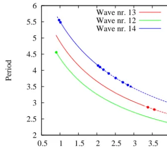
Wave nr. 13 Wave nr. 12 Wave nr. 14
Figure 11.As Fig. 10, but forn=60. For 1.01< F <2.03 three stable periodic orbits coexist. The Hopf bifurcations generating the waves with wave numbers 13, 12, and 14 occur at respectivelyF= 0.891,F=0.894, andF=0.923.
2 2.5 3 3.5 4 4.5 5 5.5
0.5 1 1.5 2 2.5 3 3.5 4
Period
F
Wave nr. 17 Wave nr. 16 Wave nr. 18
Figure 12.As Fig. 10, but forn=80. For 0.93< F <2.78 three stable periodic orbits coexist. The Hopf bifurcations generating the waves with wave numbers 17, 16, and 18 occur at respectivelyF= 0.889,F=0.894, andF=0.902.
crosses the imaginary axis and increases linearly withn, but the period tends to a finite limit asn→ ∞. ForF <0 andn odd, the first bifurcation ofxF is always a supercritical Hopf bifurcation and the periodic attractor that appears after the bifurcation is again a traveling wave. In this case the wave number equals(n−1)/2 and the period isO(4n).
Forneven andF <0 the first bifurcation ofxF is a
pitch-fork bifurcation which occurs at F = −1
2 and leads to two stable equilibria. Ifn=4k+2 for somek∈N, then each of these equilibria undergoes a Hopf bifurcation which leads to the coexistence of two stationary waves. The role of the pitchfork bifurcation is to change the mean flow which in turn changes the propagation of the wave. Ifn=4kfor some k∈N, then two pitchfork bifurcations take place atF = −1 2 andF = −3 before a Hopf bifurcation occurs, which leads to the coexistence of four stationary waves.
The occurrence of pitchfork bifurcations before the Hopf bifurcation leads to multi-stability, i.e., the coexistence of different waves for the same parameter settings. A second scenario that leads to multi-stability is via the double-Hopf bifurcation. For n=12 the equilibrium xF loses stability
through a double-Hopf bifurcation. By adding a second pa-rameterGto the Lorenz-96 model we have studied the un-folding of this codimension-2 bifurcation. Two Ne˘ımark-Sacker bifurcation curves emanating from the double-Hopf point bound a lobe-shaped region in the (F, G) plane in which two stable traveling waves with different wave num-bers coexist. For dimensions n >12 we find double-Hopf bifurcations near theF axis, which can create two multi-stability lobes intersecting each other, and in turn this can lead to the coexistence of three stable waves coexisting for G=0 and a range of F values. Hence, adding a parame-terGto the Lorenz-96 model helps to explain the dynamics, which is observed in the original model forG=0.
Our results provide a coherent overview of the spatiotem-poral properties of the Lorenz-96 model forn≥4 andF ∈R. Since the Lorenz-96 model is often used as a model for testing purposes, our results can be used to select the most appropriate values ofn andF for a particular application. The periodic attractors representing traveling or stationary waves can bifurcate into chaotic attractors representing irreg-ular versions of these waves, and their spatiotemporal proper-ties are inherited from the periodic attractor (see for example Figs. 1) and 2. This means that our results on the spatiotem-poral properties of waves apply to broader parameter ranges of the parameterF than just in a small neighborhood of the Hopf bifurcation.
The results presented in this paper also illustrate another important point: both qualitative and quantitative aspects of the dynamics of the Lorenz-96 model depend on the parity of n. This phenomenon also manifests itself in discretized par-tial differenpar-tial equations. For example, for discretizations of Burgers’ equation, Basto et al. (2006) observed that for odd degrees of freedom the dynamics were confined to an invari-ant subspace, whereas for even degrees of freedom this was not the case. For the Lorenz-96 model the parity ofnalso determines the possible symmetries of the model. We will investigate these symmetries and their consequences on bi-furcation sequences using techniques from equivariant bifur-cation theory in forthcoming work (Van Kekem and Sterk, 2017).
Code availability. The scripts used for continuation with
Appendix A
A1 Bounds on the wave number forF >0
First note that for alln≥4, with the exception ofn=7, there exists at least one integer j∈ [n
6, n
4]. Indeed, forn=4,5,6 this follows by simply takingj =1, and forn=8,9,10,11 this follows by takingj =2. Forn≥12 it follows from the fact that the interval [n
6, n
4] has a width larger than 1 and hence must contain an integer. We now claim that these ob-servations also imply that
l+(n)=arg max 0<j <n/3
f (2πj/n)∈hn 6,
n 4
i
, n6=7.
Note thatx∈ [π 3,
π
2]implies thatf (x)≥1 andx∈(0, π 3)∪ (π2,23π)implies 0< f (x) <1. Moreover,j∈ [n
6, n
4]implies that 2πjn ∈ [π
3, π
2]. Therefore, f (2πj/n) is maximized for some integerj∈ [n
6, n 4].
A2 Asymptotic period for oddnandF <0 Using L’Hospital’s 0/0 rule gives
lim
x→π/2
1
2π−x
tan(x)
= lim
x→π/2
1 2π−x
sin(x) cos(x)
= lim
x→π/2
−sin(x)+1 2π−x
cos(x) −sin(x)
=1.
Writingx=π/2−π/2nimplies
lim
n→∞
2πtan
π 2−
π 2n
4n =1,
which in particular implies that
2πtan
π
2 − π 2n
=O(4n).
A3 The number of Hopf and double-Hopf bifurcations The number of Hopf bifurcations of the equilibrium xF=
(F, . . ., F ) for a given dimensionn is exactly equal to the number of conjugate eigenvalue pairs which satisfy Theo-rem 1:
NH= (
dn
2e −1 ifn6=3m, dn
2e −2 ifn=3m,
(A1)
where we need the ceiling function ifnis odd. Note that if nis a multiple of 3, thenf (2π n3 )=g(2π n3 )=0, which does give a proper complex conjugate pair crossing the imaginary axis and hence the number of Hopf bifurcations has to be decreased by 1.
For the two-parameter system we can count the number of double-Hopf bifurcations by counting the intersections of the lines in Eq. (16). Since all the lines have a different slope, the number of such intersections is given by
NHH= 1
2NH(NH−1) =
(1 2 d
n 2e −1
dn 2e −2
ifn6=3m, 1
2 d n 2e −2
dn 2e −3
ifn=3m, (A2)
Author contributions. DvK performed the research on traveling waves and investigated the dynamics near the double-Hopf bifurca-tions. AS performed the research on stationary waves and prepared the manuscript.
Competing interests. The authors declare that they have no conflict
of interest.
Acknowledgements. The authors would like to thank the reviewers
for their useful comments and suggestions that have helped to improve this paper.
Edited by: Amit Apte
Reviewed by: Jochen Broecker and one anonymous referee
References
Avila, M., Meseguer, A., and Marqués, F.: Double Hopf bifurca-tion in corotating spiral Poiseuille flow, Phys. Fluids, 18, 064101, https://doi.org/10.1063/1.2204967, 2006.
Basnarkov, L. and Kocarev, L.: Forecast improvement in Lorenz 96 system, Nonlin. Processes Geophys., 19, 569–575, https://doi.org/10.5194/npg-19-569-2012, 2012.
Basto, M., Semiao, V., and Calheiros, F.: Dynamics in spectral so-lutions of Burgers equation, J. Comput. Appl. Math., 205, 296– 304, 2006.
Beyn, W., Champneys, A., Doedel, E., Kuznetsov, Y., Govaerts, W., and Sandstede, B.: Numerical continuation, and computation of normal forms, in: Handbook of Dynamical Systems, Volume 2, edited by: Fiedler, B., Elsevier, Amsterdam, 149–219, 2002. Danforth, C. and Yorke, J.: Making Forecasts for Chaotic
Physical Processes, Phys. Rev. Lett., 96, 144102, https://doi.org/10.1103/PhysRevLett.96.144102, 2006.
De Leeuw, B., Dubinkina, S., Frank, J., Steyer, A., Tu, X., and Van Vleck, E.: Projected shadowing-based data assimilation, arXiv preprint, arXiv:1707.09264, 2017.
Dhooge, A., Govaerts, W., Kuznetsov, Y., Meijer, H., Mestrom, W., Riet, A., and Sautois, B.: MATCONT and CL_MATCONT: Con-tinuation toolboxes in MATLAB, Gent University and Utrecht University, Gent, 2011.
Dieci, L., Jolly, M., and Van Vleck, E.: Numerical tech-niques for approximating Lyapunov exponents and their implementation, J. Comput. Nonlin. Dyn., 6, 011003, https://doi.org/10.1115/1.4002088, 2011.
Dijkstra, H.: Nonlinear physical oceanography: a dynamical sys-tems approach to the large scale ocean circulation and El Niño, 2nd Edn. Springer, Dordrecht, 2005.
Dijkstra, H., Frankcombe, L., and Von der Heydt, A.: A stochastic dynamical systems view of the Atlantic Multidecadal Oscilla-tion, Philos. T. R. Soc. A, 366, 2545–2560, 2008.
Doedel, E. and Oldeman, B.: AUTO–07p: continuation and bifurca-tion software for ordinary differential equabifurca-tions, Concordia Uni-versity, Montreal, Canada, 2007.
Feudel, U.: Complex dynamics in multistable systems, Int. J. Bifur-cat. Chaos, 18, 1607–1626, 2008.
Frank, M., Mitchell, L., Dodds, P., and Danforth, C.: Stand-ing swells surveyed showStand-ing surprisStand-ingly stable solutions for the Lorenz ’96 model, Int. J. Bifurcat. Chaos, 24, 1430027, https://doi.org/10.1142/S0218127414300274, 2014.
Frankcombe, L., Dijkstra, H., and Von der Heydt, A.: Noise induced multidecadal variability in the North Atlantic: excitation of nor-mal modes, J. Phys. Oceanogr., 39, 220–233, 2009.
Gallavotti, G. and Lucarini, V.: Equivalence of non-equilibrium en-sembles and representation of friction in turbulent flows: the Lorenz 96 model, J. Stat. Phys., 156, 1027–1065, 2014. Gray, R.: Toeplitz and circulant matrices: a review, Foundations and
Trends in Communications and Information Theory, 2, 155–239, 2006.
Hallerberg, S., Pazó, D., López, J., and Rodríguez, M.: Logarithmic bred vectors in spatiotemporal chaos: structure and growth, Phys. Rev. E, 81, 066204, https://doi.org/10.1103/PhysRevE.81.066204, 2010.
Hansen, J. and Smith, L.: The role of operational constraints in se-lecting supplementary observations, J. Atmos. Sci., 57, 2859– 2871, 2000.
Haven, K., Majda, A., and Abramov, R.: Quantifying predictability through information theory: small sample estimation in a non-Gaussian framework, J. Comput. Phys., 206, 334–362, 2005. Holland, M., Vitolo, R., Rabassa, P., Sterk, A., and Broer, H.:
Ex-treme value laws in dynamical systems under physical observ-ables, Physica D, 241, 497–513, 2012.
Holland, M., Rabassa, P., and Sterk, A.: Quantitative recurrence statistics and convergence to an extreme value distribution for non-uniformly hyperbolic dynamical systems, Nonlinearity, 29, 2355–2394, 2016.
Karimi, A. and Paul, M.: Extensive chaos in the Lorenz-96 model, Chaos, 20, 043105, https://doi.org/10.1063/1.3496397, 2010. Kuznetsov, Y.: Elements of Applied Bifurcation Theory, vol. 112 of
Applied Mathematical Sciences, 3rd edn., Springer-Verlag, New York, 2004.
Lewis, G.: Mixed-mode solutions in an air-filled differentially heated rotating annulus, Physica D, 239, 1843–1854, 2010. Lewis, G. and Nagata, W.: Double Hopf bifurcations in the
differ-entially heated rotating annulus, SIAM J. Appl. Math., 63, 1029– 1055, 2003.
Lewis, G. and Nagata, W.: Double Hopf bifurcations in the quasi-geostrophic potential vorticity equations, Dynam. Cont. Dis. Ser. B, 12, 783–807, 2005.
Lorenz, E.: Deterministic nonperiodic flow, J. Atmos. Sci., 20, 130– 141, 1963.
Lorenz, E.: Designing chaotic models, J. Atmos. Sci., 62, 1574– 1587, 2005.
Lorenz, E. and Emanuel, K.: Optimal sites for supplementary weather observations: simulations with a small model, J. Atmos. Sci., 55, 399–414, 1998.
Lorenz, E. N.: Predictability – A problem partly solved, in: Pre-dictability of Weather and Climate, edited by: Palmer, T. N. and Hagedorn, R., Cambridge University Press, Cambridge, 40–58, 2006.
Marqués, F., Lopez, J., and Shen, J.: Mode interactions in an en-closed swirling flow: a double Hopf bifurcation between az-imuthal wavenumbers 0 and 2, J. Fluid Mech., 455, 263–281, 2002.
Marqués, F., Gelfgat, A., and López, J.: Tangent double Hopf bifur-cation in a differentially rotating cylinder flow, Phys. Rev. E, 68, 016310, https://doi.org/10.1103/PhysRevE.68.016310, 2003. Moroz, I. and Holmes, P.: Double Hopf bifurcation and
quasi-periodic flow in a model for baroclinic instability, J. Atmos. Sci., 41, 3147–3160, 1984.
Orrell, D.: Role of the metric in forecast error growth: how chaotic is the weather?, Tellus A, 54, 350–362, 2002.
Orrell, D. and Smith, L.: Visualising bifurcations in high dimen-sional systems: The spectral bifurcation diagram, Int. J. Bifurcat. Chaos, 13, 3015–3027, 2003.
Orrell, D., Smith, L., Barkmeijer, J., and Palmer, T. N.: Model error in weather forecasting, Nonlin. Processes Geophys., 8, 357–371, https://doi.org/10.5194/npg-8-357-2001, 2001.
Ott, E., Hunt, B., Szunyogh, I., Zimin, A., Kostelich, E., Corazza, M., Kalnay, E., Patil, D., and Yorke, J.: A local ensem-ble Kalman filter for atmospheric data assimilation, Tellus A, 56, 415–428, 2004.
Pazó, D., Szendro, I., López, J., and Rodríguez, M.: Structure of characteristic Lyapunov vectors in spatiotemporal chaos, Phys. Rev. E, 78, 016209, 1–9, 2008.
Read, P., Bel, M., Johnson, D., and Small, R.: Quasi-periodic and chaotic flow regimes in a thermally driven, rotating fluid annulus, J. Fluid Mech., 238, 599–632, 1992.
Simonnet, E., Ghil, M., Ide, K., Temam, R., and Wang, S.: Low-frequency variability in shallow-water models of the wind-driven ocean circulation. Part I: steady-state solution, J. Phys. Oceanogr., 33, 712–728, 2003a.
Simonnet, E., Ghil, M., Ide, K., Temam, R., and Wang, S.: Low-frequency variability in shallow-water models of the wind-driven ocean circulation. Part II: time-dependent solutions, J. Phys. Oceanogr., 33, 729–752, 2003b.
Stappers, R. and Barkmeijer, J.: Optimal linearization trajectories for tangent linear models, Q. J. Roy. Meteor. Soc., 138, 170–184, 2012.
Sterk, A. and Van Kekem, D.: Predictability of extreme waves in the Lorenz-96 model near intermittency and quasi-periodicity, Com-plexity, 2017, 9419024, https://doi.org/10.1155/2017/9419024, 2017.
Sterk, A., Vitolo, R., Broer, H., Simó, C., and Dijkstra, H.: New nonlinear mechanisms of midlatitude atmospheric low-frequency variability, Physica D, 239, 702–718, 2010.
Sterk, A. E., Holland, M. P., Rabassa, P., Broer, H. W., and Vitolo, R.: Predictability of extreme values in geo-physical models, Nonlin. Processes Geophys., 19, 529–539, https://doi.org/10.5194/npg-19-529-2012, 2012.
Te Raa, L. and Dijkstra, H.: Instability of the thermohaline ocean circulation on interdecadal timescales, J. Phys. Oceanogr., 32, 138–160, 2002.
Tian, Y., Weeks, E., Ide, K., Urbach, J., Baroud, C., Ghil, M., and Swinney, H.: Experimental and numerical studies of an eastward jet over topography, J. Fluid Mech., 438, 129–157, 2001. Trevisan, A. and Palatella, L.: On the Kalman Filter error covariance
collapse into the unstable subspace, Nonlin. Processes Geophys., 18, 243–250, https://doi.org/10.5194/npg-18-243-2011, 2011. Van Kekem, D. and Sterk, A.: Symmetries in the Lorenz-96 model,
arXiv:1712.05730, 2017.
Van Kekem, D. and Sterk, A.: Travelling waves and their bifurca-tions in the Lorenz-96 model, Physica D, 367, 38–60, 2018. Wolfram Research, Inc.: Mathematica, Version 11.0.1.0,