https://doi.org/10.5194/esd-8-1061-2017 © Author(s) 2017. This work is distributed under the Creative Commons Attribution 4.0 License.
Equatorial Atlantic interannual variability and its relation
to dynamic and thermodynamic processes
Julien Jouanno1, Olga Hernandez2,1, and Emilia Sanchez-Gomez3
1LEGOS, Université de Toulouse, CNES, CNRS, IRD, UPS, Toulouse, France
2Mercator-Océan, Ramonville Saint Agne, France
3CECI/CERFACS, Toulouse, France
Correspondence to:Julien Jouanno ([email protected])
Received: 7 June 2017 – Discussion started: 18 July 2017 Accepted: 30 October 2017 – Published: 30 November 2017
Abstract. The contributions of the dynamic and thermodynamic forcing to the interannual variability of the equatorial Atlantic sea surface temperature (SST) are investigated using a set of interannual regional simula-tions of the tropical Atlantic Ocean. The ocean model is forced with an interactive atmospheric boundary layer, avoiding damping toward prescribed air temperature as is usually the case in forced ocean models. The model
successfully reproduces a large fraction (R2=0.55) of the observed interannual variability in the equatorial
At-lantic. In agreement with leading theories, our results confirm that the interannual variations of the dynamical forcing largely contributes to this variability. We show that mean and seasonal upper ocean temperature biases, commonly found in fully coupled models, strongly favor an unrealistic thermodynamic control of the equatorial Atlantic interannual variability.
1 Introduction
The main mode of interannual variability in the tropical At-lantic is generally referred to as AtAt-lantic Equatorial Mode or Atlantic Niño (Zebiak, 1993; Richter et al., 2013). It con-sists in anomalies of sea surface temperature (SST) along the Equator with largest variability during boreal summer (June– July–August; JJA) and a spatial extent that covers the cold tongue area (e.g., see Lübbecke and McPhaden, 2013).
Many observational or modeling studies suggested that wind forced ocean wave dynamics play a crucial role in controlling the equatorial Atlantic interannual variability. Early work by Hirst and Hastenrath (1983) and Servain et al. (1982) show evidence of remote forcing of eastern SST anomalies by Atlantic zonal winds in the western part of the basin, the link between the two regions being provided by the propagation of equatorial Kelvin waves and their influ-ence on the equatorial thermocline depth. Using observations and intermediate complexity coupled model, Zebiak (1993) suggested that the delayed oscillator mechanism is the main mechanism underlying the oscillating interannual variabil-ity in the Atlantic. Ocean dynamics are implicit to the
de-layed oscillator mechanism: Rossby and Kelvin waves pro-vide the phase-transition mechanism for the oscillator cy-cle. The analysis of reanalysis products by Lübbecke and McPhaden (2017) confirms that the Bjerknes feedback is op-erative in the tropical Atlantic (Keenlyside and Latif, 2007). The mentioned studies show a thermocline depth–SST rela-tionship in the eastern part of the equatorial Atlantic that is as strong or even stronger than for the Pacific. The analysis by Foltz and McPhaden (2010) and Burmeister et al. (2016) also revealed the key role of the reflection of planetary Rossby wave into an equatorial Kelvin wave in precondi-tioning, through thermocline rising, an anomalously strong surface cooling in the Atlantic cold tongue area during sum-mer 2009. Planton et al. (2017) also highlight the importance of eastward-propagating equatorial Kelvin waves, advection and mixing in controlling the interannual variability of the central equatorial temperatures.
Figure 1. Climatological SST (◦C) in June–July–August for the period 1979–2015 from TropFlux(a)and anomalies of SST between simulation REF and TropFlux(b)and between simulation BIASED and TropFlux(c). Zonal sections of June–July–August temperatures (◦C) averaged between 2◦S and 2◦N from ISAS observations(d), REF(e)and BIASED(f).
contrasted warm (2002) and cold tongue events (2005), Hor-mann and Brandt (2009) found a weak impact of the equa-torial Kelvin wave on the SST of the equaequa-torial Atlantic. Richter et al. (2013) show that some equatorial Atlantic warm events are not explained by equatorial dynamics but are due to horizontal advection of off-equatorial warm tem-perature anomalies. More recently, the analysis by Nnamchi et al. (2015) from a set of CMIP5 simulations including full coupled global circulation model (GCM) and slab GCM sug-gests that the Atlantic Niño variability, as resolved by state-of-the-art coupled models, mainly depends on the
thermody-namic component (R2=0.92).
Despite a growing understanding of the processes involved in the control of equatorial Atlantic interannual variability, these recent studies challenge its functioning and ask for a better quantification of the relative contributions of the ther-modynamic and dynamic forcing, as well as how both contri-butions are represented in models comparing to observations. This is the main objective of our study. We will examine how much the ratio between the two contributions depends on the upper ocean seasonal bias generally found in coupled mod-els. The paper is organized as follows. Section 2 presents the simulation strategy. Section 3 is dedicated to quantify the
dy-namic and thermodydy-namic contributions using mixed-layer heat budget in long-term simulations (1979–2015), together with comparison between simulations forced with climato-logical or interannually varying wind stress. Section 4 dis-cusses how seasonal biases impact the equatorial response to interannual anomalies of the atmospheric forcing. Conclu-sions are given in Sect. 5.
2 Simulations and data
2.1 The regional configuration
The numerical code is the oceanic component of the Nucleus for European Modeling of the Ocean program (NEMO3.6, Madec and the NEMO Team, 2016). It solves the three di-mensional primitive equations in curvilinear coordinates
dis-cretized on aCgrid and fixed vertical levels (zcoordinate).
The model configuration consists of a grid with 1/4◦
hori-zontal resolution (1x,1y∼25 km) encompassing the
diffusion parameterized as a Laplacian isopycnal diffusion, with a coefficient of 300 m2s−1. Horizontal diffusion of
mo-mentum is implicit since a third-order advection scheme UP3 is employed. The vertical diffusion coefficients are given by
a generic length scale (GLS) scheme with ak−εturbulent
closure. Bottom friction is quadratic with a bottom drag
co-efficient of 10−3and partial slip boundary conditions are
ap-plied at the lateral boundaries. The free surface is solved us-ing a time-splittus-ing technique with the barotropic part of the dynamical equations integrated explicitly.
Horizontal velocity, temperature, salinity and sea level are specified at the lateral boundaries of model domain using cli-matological conditions computed from 1992 to 2012 daily outputs of the MERCATOR global reanalysis GLORYS2V3 (Ferry et al., 2012). Very similar configurations of this re-gional setup, using an earlier version of the NEMO model, have been used to investigate mechanisms of variability of the SST (Jouanno et al., 2011, 2013) or sea surface salinity (Da-Allada et al., 2017) in the tropical Atlantic.
2.2 Surface forcing strategy
At the surface, the air–sea fluxes of momentum, heat and freshwater are computed using bulk formulae (Large and Yeager, 2009). The specification of atmospheric conditions (air temperature, humidity, and wind speed) when forcing an ocean model with bulk formulae acts to restore the SST to-ward prescribed air temperature. The method constrains the model solution toward further realism, but as a main draw-back, a realistic representation of the SST interannual vari-ability cannot guarantee that the correct processes are at play in the model. This damping also prevents the use of sensi-tivity experiments to evaluate the impact of the interannual variability of atmospheric variables other than the air tem-perature.
To partly overcome this issue, the evolution of the atmo-spheric boundary layer temperature and humidity are com-puted with the simplified atmospheric boundary layer model CheapAML (Deremble et al., 2013), letting the wind field be prescribed. The model consists of two prognostic equa-tions for atmospheric temperature and humidity. The fraction of humidity entrained at the top of the atmospheric bound-ary layer is taken as 0.25 following Seager et al. (1995). The boundary layer height is prescribed using the plane-tary boundary layer height climatology derived from ERA-Interim reanalysis from Von Engeln and Teixeira (2013).
2.3 Simulations
We carried out four simulations referred henceforth as REF,
REF-τclim, BIASED, and BIASED-τclim. The model
refer-ence simulation (REF) is forced with DFS5.2 (Drakkar Forc-ing Set; Dussin et al., 2016) which is based on corrected ERA-Interim reanalysis fields, and consists of 3 h fields of wind and daily fields of long- and shortwave radiation and
precipitation. The shortwave radiation forcing is modulated on-line by a theoretical diurnal cycle.
Experiment REF-τclimis forced with monthly
climatologi-cal wind stress. The modified wind stress is used as a bound-ary condition for both the momentum equations and the ver-tical turbulence closure scheme, but the surface fluxes of heat and freshwater remain forced by the interannual data. This strategy allows for specifically removing the dynamical contribution of the interannual winds. However, thermody-namic contributions of wind variability (i.e., latent and sen-sible heat) are allowed to vary interannually.
A second set of simulations (BIASED and BIASED-τclim)
has been performed, in which the seasonal cycle of the prescribed atmospheric variables (wind, longwave radiation, shortwave radiation and precipitation) is replaced by the sonal cycle simulated by a coupled model. The biased sea-sonal cycle we used in this study is issued from an ensem-ble of 10 members performed with the CNRM-CM5 model for the period 1979–2012 (Voldoire et al., 2011). The sea-sonal cycles have been isolated using harmonic analysis and the CNRM-CM5 data were interpolated on the DFS5.2 grid. This ensemble belongs to the 20th century historical experi-ment available in the CMIP5 (Coupled Model Intercompar-ison Phase 5) dataset. CNRM-CM5 model exhibit a marked equatorial Atlantic warm SST bias typical of the CMIP5 en-semble mean warm bias (Richter and Xie, 2008; Voldoire et al., 2014). Similarly to REF and REF-τclim, a set of two ocean
stand-alone simulations, referred to as BIASED (forced by the interannual forcing biased to CNRM-CM5 climatology)
and BIASED-τclim (forced with biased climatological wind
stress from CNRM-CM5), have been performed.
All the simulations are run from 1958 to 2015 and daily means from 1979 to 2015 are analyzed in this study.
2.4 Model mixed-layer heat balance
The mixed-layer heat content equation can be written as (see Menkes et al., 2006, or Jouanno et al., 2011)
< ∂tT > | {z }
TOT
= −< u∂xT >−< u∂yT >+<Dl(T)>
| {z }
HOR
−< w∂zT >−
1
h ∂h
∂t (< T >−Tz=−h)+
1
h(Kz∂zT)z=−h
| {z }
VER
+Q
∗+Q
s(1−fz=−h)
ρ0Cph
| {z }
FOR
with
<·>=1
h
0 Z
−h
·∂z,
withT the model potential temperature, (u,v,w) the velocity
ver-tical diffusion coefficient for tracers, andhthe mixed-layer
depth. Here,Q∗andQsare respectively the non-penetrative
(latent, sensible and longwave heat fluxes) and penetrative components of the air–sea heat flux (shortwave radiation),
andf z= −his the fraction of the shortwave radiation that
reaches the mixed-layer depth (MLD). The MLD is defined as the depth where the density increase compared to density
at 10 m equals 0.03 kg m−3. TOT represents the total
mixed-layer temperature tendency; HOR the tendency associated with horizontal processes including advection and lateral dif-fusion; VER the tendency associated with vertical processes including the vertical advection, the turbulent flux at the base of the mixed layer, and the mixed-layer temperature varia-tions due to the displacements of the mixed-layer base; and finally FOR is the air–sea heat flux storage in the mixed layer. This equation will be used to diagnose the origin of the heat content variations in the mixed layer in our simulations.
2.5 Observations
The four simulations will be compared to several observa-tional products. Observations for SST and air–sea fluxes are from TropFlux (Praveen Kumar et al., 2012). Data are avail-able for the period 1979–2015 and are based on bias and am-plitude corrections from ERA-Interim and ISCCP shortwave data. Correction were performed on the basis of compari-son with the Global Tropical Moored Buoy Array, so these are specific to the tropical region. Monthly fields of ISAS-13 temperature (Gaillard et al., 2016), available for the
pe-riod 2004–2012 at 1/4◦spatial resolution, are also used. In
the tropical Atlantic, they consist of an optimal interpola-tion of observainterpola-tions from Argo profiling floats and PIRATA moorings.
3 Dynamic vs. thermodynamic control of the interannual variability
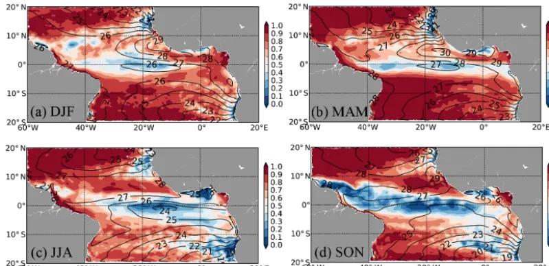
A key feature of the tropical Atlantic variability is the so-called Atlantic cold tongue (Fig. 1a), whose extension and strength peak in June–July–August (JJA), as a consequence of seasonal surface cooling driven by subsurface processes that develop along and south of the Equator (e.g., Wade et al., 2011; Jouanno et al., 2011). In JJA, the mean SST in REF compares well with SST from TropFlux (Fig. 1b). There is
a warm bias (∼1.5◦C) located in the Southern Hemisphere
along the African coast, but it is weak compared to the warm bias found in state-of-the-art coupled models which can
an-nually exceed 5◦C (e.g., Voldoire et al., 2014; Richter and
Xie, 2008; Richter et al., 2012b). At the equator, the seasonal formation of the cold tongue is well reproduced in the REF
simulation, with an equatorial bias lower than 1◦C (Fig. 1b).
At the subsurface, the observed east–west tilt of the thermo-cline (Fig. 1d) is well reproduced in REF (Fig. 1e); however, the ocean model thermocline is not as sharp as in the observa-tions. This is a long-lasting problem of equatorial modeling.
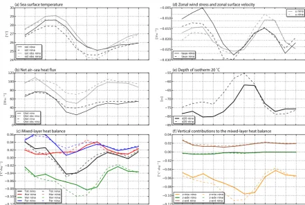
(a) ATL3 temperatures in JJA [°C]
(b) ATL3 temperature STD [°C]
Figure 2.(a)Time series of the Atl3 index (SST averaged in JJA between 20◦W–0◦N and 3◦S–3◦N) obtained from TropFlux and simulations. Monthly standard deviation of Atl3 SST using data from 1979 to 2015. Units are degrees Celcius.
Possible implications of this bias for the representation of the interannual variability of the surface temperature are out of the scope of this study but would deserve further attention.
The year-to-year evolution of JJA SST averaged over Atl3
(between 20◦W–0◦ and 3◦S–3◦N as defined in Zebiak,
1993) is shown in Fig. 2a. REF simulation reproduces well the amplitude of the SST present in the observations
(regres-sion slope between REF and observations;a=0.86) and also
a substantial fraction of the observed interannual variability
(R2=0.55), with most of the model Atlantic Niño and Niña
events in phase with observations. The removal of the
inter-annual variability of the wind stress in REFτclim clearly
re-duces the amplitude (a=0.26 andR2=0.27 between REF
and REFτclim) of the interannual variability (Fig. 2a) and
weakens the correlation with the observations (R2=0.25).
This suggests that the interannual dynamical forcing actively participates in the control of the Atlantic Niño and Niña events.
The interannual variance of Atl3 shows a marked seasonal cycle with maximum of variance in May–June–July in the observations (Fig. 2b). This seasonal cycle is slightly shifted in REF, with interannual variability in March–April stronger than the observed interannual variability. More interestingly, we note that the interannual standard deviation is drastically reduced when removing the interannual variability of the
wind stress (REFτclim, Fig. 2b). This suggests that the
(a) Sea surface temperature
(b) Net air–sea heat ux
(c) Mixed-layer heat balance
(d) Zonal wind stress and zonal surface velocity
(e) Depth of isotherm 20 ˚C
(f ) Vertical contributions to the mixed-layer heat balance
Figure 3.Composite seasonal evolution of variables from REF and observations averaged over Atl3 for Niño (continuous lines) and Niña years (dashed lines):(a)surface temperatures from model and TropFlux,(b)net air–sea heat flux from model and TropFlux;(c)mixed-layer heat budget contributions as defined in Eq. (1);(d)model zonal wind stress and zonal surface current;(e)depth of the isotherm 20◦C; and (f)mixing, advection and entrainment contributions to the mixed-layer contribution VER. Niño and Niña years were selected using SST from TropFlux using the methodology described in Lübbecke and McPhaden (2017).
In order to get further insight into the nature of the dynam-ical processes at play during the warm and cold events, we performed a composite analysis of 8 Niño and 7 Niña years selected over the period 1979–2015. Following the method-ology proposed in Lübbecke and McPhaden (2017), the Niño and Niña years are selected when detrended interannual SST anomalies from TropFlux averaged over Atl3 exceed the standard deviation of the time series for at least 2 months be-tween May and September. Lübbecke and McPhaden (2017) have shown large symmetry of the Niño and Niña events in the Atlantic in terms of development and processes, so we will focus on the anomalies between both types of events.
In both the model and observations, the seasonal evolu-tion of the SST in Atl3 during Niño and Niña years indicates that, on average, the temperature anomalies form early in the season (in March–April) and start to vanish from around August–September (Fig. 3a). This is consistent with find-ings by Lübbecke and McPhaden (2017). There is a large
(∼30 W m−2) difference between model and TropFlux
es-timates of the mean net air–sea heat flux at the sea surface (Fig. 3b). However, this difference is within the range of the differences found between state-of-the-art air–sea heat flux products in equatorial cold tongue regions (e.g., see Fig. 16
of Praveen Kumar et al., 2012, for Nino3). Most importantly, both the model and observation show that the net heat flux acts toward a reduction in the temperature anomalies from May to August. This further indicates that the thermody-namic forcing is not the leading mechanism to explain the interannual variability of Atl3 in JJA.
dur-Figure 4.Coefficient of determination (R2) between REF and REF-τclimseasonal SST time series.R2has been computed at each model grid point using data from 1979 to 2015 and with temperatures averaged over four seasons: December–January–February(a), March–April– May(b), June–July–August(c)and September–October–November(d). Values close to 1 indicate that seasonal SSTs in the two simulations are highly correlated, suggesting a thermodynamic control of the interannual variability, while values close to 0 indicate that seasonal SSTs in the two simulations are uncorrelated, suggesting a dynamic control of the interannual variability.
ing this period, (i) the thermocline is getting closer to the surface (Fig. 3e) and, above all, and (ii) the westward surface current is intensified (Fig. 3d), providing an efficient source of shear-driven turbulence between the mixed layer and the thermocline below (e.g., see Jouanno et al., 2011). Interan-nual anomalies of the surface currents could also participate to anomalies of vertical diffusion by increasing the levels of turbulence with the Equatorial Undercurrent below, but the lack of agreement between anomalies of zonal surface ve-locity (Fig. 3d) and anomalies of vertical diffusion (Fig. 3f) suggests they do not have a first-order influence.
Spatial maps of correlation between time series of season
average surface temperatures from REF and REF-τclim are
shown in Fig. 4. Values of R2close to 1 suggest that
ther-modynamic processes play a dominant role in the interan-nual variability of the SST, while values close to 0 suggest that the variability is controlled by the dynamical component. The correlation maps indicate that the interannual variabil-ity of the SST in the equatorial and coastal upwelling areas is mainly controlled by dynamics, while in the subtropical gyres thermodynamic play a dominant role. At the equator, the influence of the dynamics is larger in JJA and SON, most probably due to shallow thermocline and intensified tropical wave instability respectively.
4 Impact of seasonal biases on Atlantic Niño and Niña event representation
Our results are at odds with the results by Nnamchi et al. (2015), who suggested a thermodynamic control of the equatorial interannual SST variability. Most of the CMIP5
models simulate a warm bias at the Equator (Richter et al., 2012b), and our hypothesis is that such bias deeply modifies the response to interannual winds in such a way that it favors a thermodynamic response. To test this hypothesis we ana-lyzed our set of simulations forced with biased atmospheric variables issued from the CNRM-CM5 coupled model
(BI-ASED and BI(BI-ASED-τclim).
The simulation BIASED reproduces a warm bias in the
cold tongue area that reaches 7◦C near the African coast in
JJA (Fig. 1c) with a spatial structure typical of the bias found in coupled models in the region (e.g., Richter et al., 2014).
The annual mean bias (not shown) reaches 5◦C and
resem-bles the bias of CNRM-CM5 coupled model (Voldoire et al., 2014). In BIASED, there is no more east–west tilt of the ther-mocline (Fig. 1d), and the therther-mocline is even more diffuse than in REF. BIASED is forced with the same interannual anomalies of winds, downward radiative fluxes and precip-itation as in REF, but the interannual responses of the sur-face temperature of the two simulations are very different. First, the SST interannual variability is no more correlated
with TropFlux (Fig. 2a;R2=0.02). Second, the maximum of
variance is shifted toward boreal spring (Fig. 2b). This high-lights how much the interplay between interannual anoma-lies and the seasonal variability is critical in the functioning of the interannual Atlantic equatorial variability.
Unlike the results obtained from the reference simulations
(R2between REF and REF-τclimof 0.27), removing the
inter-annual variability of the wind stress in BIASED has a much weaker impact on the interannual variability of Atl3 in JJA as shown by the comparison between BIASED and
be-Figure 5.As Fig. 3 but using BIASED simulation. Here, Niño and Niña years were selected following the same method as in Fig. 3 but using Atl3 SSTs from BIASED, so they do not necessarily coincide with observed Niño and Niña years.
tween BIASED and BIASED-τclim suggests that
thermody-namic processes mainly drive the equatorial interannual vari-ability in BIASED. This is confirmed by the mixed-layer heat balance of Niño and Niña events (Fig. 5) that illustrates how the interannual variability is driven almost entirely by the air– sea heat fluxes, with the subsurface vertical processes now damping the Niño and Niña anomalies. The seasonal corre-lation maps indicate that the dynamics control of the interan-nual SSTs in BIASED in the equatorial and coastal upwelling areas is reduced for all the seasons and is almost absent in DJF and MAM (Fig. 6).
5 Discussion and conclusion
The objective of this study was to clarify the role of the dy-namical processes in controlling the interannual variability of the tropical Atlantic SSTs and how they are represented in ocean alone and fully coupled models. For the stand-alone ocean model, we overcome the difficulties inherent to the use of a forced ocean model when analyzing processes of interannual variability by coupling the ocean model with an atmospheric boundary layer model that provides interactive air temperature and humidity. In addition to a better represen-tation of the air–sea exchanges, such a strategy allowed for proper assessment of the sensitivity of the interannual vari-ability of the equatorial Atlantic surface temperature to the interannual variability of the equatorial wind stress.
Figure 6.Coefficient of determination (R2) between BIASED and BIASED-τclimseasonal SST time series, as in Fig. 4.
seasonal turbulent mixed-layer cooling is at its maximum. This is in agreement with results by Burls et al. (2012) sug-gesting that the interannual variability in the equatorial At-lantic can be seen as a modulation of the seasonal cycle.
From a climate modeling perspective, and although a set of fully coupled simulations would be required to confirm our findings, our results are suggestive that a reduction in the mean and seasonal model biases in the tropical Atlantic (in particular from the atmospheric component) would strongly benefit to the representation of the interannual variability. The variability of the Atlantic cold tongue exerts a signifi-cant influence on the climate of the surrounding regions and more specifically on the West African monsoon (Okumura and Xie, 2004; Caniaux et al., 2011) or on rainfall variability in the northeast of Brazil (Kushnir et al., 2006). In terms of predictability of these phenomena on a seasonal timescale, our results suggest that the ability of the climate models to maintain a realistic stratification and east–west tilt of the thermocline is key in correctly representing the response of the summer coupled system to spring wind anomalies. We also anticipate that a good representation of the dynamical processes in the Atlantic equatorial region will have an im-pact on the dynamics of the meridional overturning circu-lation (MOC) in coupled climate models. It seems that the MOC is indeed very sensitive to equatorial processes such as precipitation biases (Liu et al., 2017): excessive precipita-tion events near the Equator tend to over-stabilize the MOC, which is often an issue when trying to assess the stability of climate change scenarios.
Data availability. Model outputs are available on demand or can be reproduced by using the ocean code NEMO3.6_stable-rev4791 (http://forge.ipsl.jussieu.fr/nemo/wiki/Users).
Competing interests. The authors declare that they have no con-flict of interest.
Acknowledgements. This study was supported by EU FP7/2007-2013 under grant agreement no. 603521, project PREFACE. Computing facilities were provided by GENCI project GEN7298. Special thanks to Bruno Deremble for a careful reading of the manuscript and his assistance in porting and tuning the interactive atmospheric boundary layer CheapAML. Finally, we are grateful to the three anonymous reviewers for helpful comments on the manuscript.
Edited by: Valerio Lucarini
Reviewed by: three anonymous referees
References
Burls, N. J., Reason, C. J., Penven, P., and Philander, S. G.: Ener-getics of the tropical Atlantic zonal mode, J. Climate, 25, 7442– 7466, https://doi.org/10.1175/JCLI-D-11-00602.1, 2012. Burmeister, K., Brandt, P., and Lübbecke, J. F.:
Revisit-ing the cause of the eastern equatorial Atlantic cold event in 2009, J. Geophys. Res.-Oceans, 121, 4777–4789, https://doi.org/10.1002/2016JC011719, 2016.
Caniaux, G., Giordani, H., Redelsperger, J. L., Guichard, F., Key, E., and Wade, M.: Coupling between the Atlantic cold tongue and the West African monsoon in boreal spring and summer, J. Geophys. Res.-Oceans, 116, C04003, https://doi.org/10.1029/2010JC006570, 2011.
Deremble, B., Wienders, N., and Dewar, W. K.: CheapAML: A simple, atmospheric boundary layer model for use in ocean-only model calculations, Mon. Weather Rev., 141, 809–821, 2013. Dussin, R., Barnier, B., and Brodeau, L.: Up-dated description of
the DFS5 forcing data set: The making of Drakkar forcing set DFS5, DRAKKAR/MyOcean Rep. 01-04-16, Lab. of Glaciol. and Environ. Geophys., Grenoble, France, 2016.
Ferry, N., Parent, L., Garric, G., Bricaud, C., Testut, C.-E., Gal-loudec, O. L., Lellouche, J.-M., Drevillon, M., Greiner, E., Barnier, B., Molines, J.-M., Jourdain, N. C., Guinehut, S., Ca-banes, C., and Zawadzki, L.: GLORYS2V1 global ocean reanal-ysis of the altimetric era (1992–2009) at mesoscale, Mercator Quart. Newslett., 44, 29–39, 2012.
Foltz, G. R. and McPhaden, M. J.: Interaction between the Atlantic meridional and Niño modes, Geophys. Res. Lett., 37, L18604, https://doi.org/10.1029/2010GL044001, 2010.
Gaillard, F., Reynaud, T., Thierry, V., Kolodziejczyk, N., and von Schuckmann, K.: In-situ based reanalysis of the global ocean temperature and salinity with ISAS: Variability of the heat content and steric height, J. Climate, 29, 1305–1323, https://doi.org/10.1175/JCLI-D-15-0028.1, 2016.
Hirst, A. C. and Hastenrath, S.: Atmosphere–ocean mechanisms of climate anomalies in the Angola-tropical Atlantic sector, J. Phys. Oceanogr., 13, 1146–1157, 1983.
Hormann, V. and Brandt, P.: Upper equatorial Atlantic vari-ability during 2002 and 2005 associated with equato-rial Kelvin waves, J. Geophys. Res.-Oceans, 114, C03007, https://doi.org/10.1029/2008JC005101, 2009.
Jouanno, J., Marin, F., du Penhoat, Y., Sheinbaum, J., and Mo-lines, J. M.: Seasonal heat balance in the upper 100 m of the equatorial Atlantic Ocean, J. Geophys. Res., 116, C09003, https://doi.org/10.1029/2010JC006912, 2011.
Jouanno, J., Marin, F., du Penhoat, Y., Sheinbaum, J., and Molines, J. M.: Intraseasonal modulation of the surface cooling in the Gulf of Guinea, J. Phys. Oceanogr., 43, 382–401, 2013.
Keenlyside, N. and Latif, M.: Understanding Equatorial Atlantic In-terannual Variability, J. Climate, 20, 131–142, 2007.
Kushnir, Y., Robinson, W. A., Chang, P., and Robertson, A. W.: The physical basis for predicting Atlantic sector seasonal-to-interannual climate variability, J. Climate, 19, 5949–5970, 2006. Large, W. G. and Yeager, S.: The global climatology of an interan-nually varying air–sea flux data set, Clim. Dynam., 33, 341–364, https://doi.org/10.1007/s00382-008-0441-3, 2009.
Liu, W., Xie, S.-P., Liu, Z., and Zhu, J.: Overlooked pos-sibility of a collapsed Atlantic Meridional Overturning Circulation in warming climate, Sci. Adv., 3, e1601666, https://doi.org/10.1126/sciadv.1601666, 2017.
Lübbecke, J. F. and McPhaden, M. J.: A comparative stability anal-ysis of Atlantic and Pacific Niño modes, J. Climate, 26, 5965– 5980, https://doi.org/10.1175/JCLI-D-12-00758.1, 2013. Lübbecke, J. F. and McPhaden, M. J.: Symmetry of the
Atlantic Niño mode, Geophys. Res. Lett., 44, 965–973, https://doi.org/10.1002/2016GL071829, 2017.
Madec, G. and the NEMO Team: NEMO ocean engine, Note du Pôle de Modélisation 27, Inst. Pierre-Simon Laplace, Paris, 2016. Menkes, C. E., Vialard, J., Kennan, S. C., Boulanger, J.-P., and Madec, G.: A modeling study of the impact of tropical instabil-ity waves on the heat budget of the eastern equatorial Pacific, J. Phys. Oceanogr., 36, 847–865, 2006.
Nnamchi, H. C., Li, J., Kucharski, F., Kang, I.-S., Keenly-side, N. S., Chang, P., and Farneti, R.: Thermodynamic controls of the Atlantic Niño, Nat. Commun., 6, 8895, https://doi.org/10.1038/ncomms9895, 2015.
Okumura, Y. and Xie, S. P.: Interaction of the Atlantic equatorial cold tongue and the African monsoon, J. Climate, 17, 3589– 3602, 2004.
Planton, Y., Voldoire, A., Giordani, H., and Caniaux, G.: Main pro-cesses of the Atlantic cold tongue interannual variability, Clim. Dynam., https://doi.org/10.1007/s00382-017-3701-2, in press, 2017.
Praveen Kumar, B., Vialard, J., Lengaigne, M., Murty, V. S. N., and Mcphaden, J. M.: TropFlux: air–sea fluxes for the global tropical oceans – description and evaluation, Clim. Dynam., 38, 1521– 1543, 2012.
Richter, I. and Xie, S. P.: On the origin of equatorial Atlantic biases in coupled general circulation models, Clim. Dynam., 31, 587– 598, 2008.
Richter, I., Xie, S. P., Wittenberg, A. T., and Masumoto, Y.: Trop-ical Atlantic biases and their relation to surface wind stress and terrestrial precipitation, Clim. Dynam., 38, 985–1001, 2012a. Richter, I., Xie, S. P., Behera, S. K., Doi, T., and
Ma-sumoto, Y.: Equatorial Atlantic variability and its relation to mean state biases in CMIP5, Clim. Dynam., 42, 171, https://doi.org/10.1007/s00382-012-1624-5, 2012b.
Richter, I., Behera, S. K., Masumoto, Y., Taguchi, B., Sasaki, H., and Yamagata, T.: Multiple causes of interannual sea surface temperature variability in the equatorial Atlantic Ocean, Nat. Geosci., 6, 43–47, https://doi.org/10.1038/ngeo1660, 2013. Richter, I., Behera, S. K., Doi, T., Taguchi, B., Masumoto, Y., and
Xie, S. P.: What controls equatorial Atlantic winds in boreal spring?, Clim. Dynam., 43, 3091–3104, 2014.
Seager, R., Blumenthal, M., and Kushnir, Y.: An advective atmo-spheric mixed layer model for ocean modeling purposes: Global simulation of surface heat fluxes, J. Climate, 8, 1951–1964, 1995. Servain, J., Picaut, J., and Merle, J.: Evidence of remote forcing in the equatorial Atlantic Ocean, J. Phys. Oceanogr., 12, 457–463, 1982.
Voldoire, A., Sanchez-Gomez, E., Salas y Melia, D., Decharme, B., Cassou, C., Senesi, S., Valcke, S., Beau, I., Alias, A., Cheval-lier, M., Deque, M., Deshayes, J., Douville, H., Fernandez, E., Madec, G., Maisonnave, E., Moine, M.-P., Planton, S., Saint-Martin, D., Szopa, S., Tyteca, S., Alkama, R., Belamari, S., Braun, A., Coquart, L., and Chauvin, F.: The CNRM-CM5.1 global climate model: Description and basic evaluation, Clim. Dynam., 40, 2091–2121, 2011.
Voldoire, A., Claudon, M., Caniaux, G., Giordani, H., and Roehrig, R.: Are atmospheric biases responsible for the tropical Atlantic SST biases in the CNRM-CM5 coupled model?, Clim. Dynam., 43, 2963–2984, 2014.
Von Engeln, A. and Teixeira, J.: A planetary boundary layer height climatology derived from ECMWF reanalysis data, J. Climate, 26, 6575–6590, 2013.
Wade, M., Caniaux, G., and du Penhoat, Y.: Variability of the mixed layer heat budget in the eastern equatorial Atlantic dur-ing 2005–2007 as inferred usdur-ing Argo floats, J. Geophys. Res., 116, C08006, https://doi.org/10.1029/2010JC006683, 2011. Zebiak, S. E.: Air-sea interaction in the equatorial Atlantic region,