Two-dimensional prognostic experiments for fast-ﬂowing ice streams from the Academy of Sciences Ice Cap

(1)

www.earth-syst-dynam.net/8/283/2017/ doi:10.5194/esd-8-283-2017

Two-dimensional prognostic experiments for fast-flowing

ice streams from the Academy of Sciences Ice Cap

Yuri V. Konovalov and Oleg V. Nagornov

Mathematical Department, National Research Nuclear University MEPhI (Moscow Engineering Physics Institute), Kashirskoe shosse, 31, 115409, Moscow, Russian Federation

Correspondence to:Yuri V. Konovalov ([email protected])

Received: 13 October 2015 – Discussion started: 3 November 2015 Revised: 11 December 2016 – Accepted: 20 March 2017 – Published: 20 April 2017

Abstract. Prognostic experiments for fast-flowing ice streams on the southern side of the Academy of Sciences

Ice Cap on Komsomolets Island, Severnaya Zemlya archipelago, were undertaken in this study. The experiments were based on inversions of basal friction coefficients using a two-dimensional flow-line thermocoupled model and Tikhonov’s regularization method. The modeled ice temperature distributions in the cross sections were obtained using ice surface temperature histories that were inverted previously from borehole temperature profiles derived at the summit of the Academy of Sciences Ice Cap and the elevational gradient of ice surface temperature

changes (about 6.5◦C km−1). Input data included interferometric synthetic aperture radar (InSAR) ice surface

velocities, ice surface elevations, and ice thicknesses obtained from airborne measurements, while the surface mass balance was adopted from previous investigations for the implementation of both the forward and inverse problems. The prognostic experiments revealed that both ice mass and ice stream extent declined for the reference

time-independent surface mass balance. Specifically, the grounding line retreated: (a) along the B–B0 flow line

from∼40 to∼30 km (the distance from the summit), (b) along the C–C0flow line from∼43 to∼37 km, and

(c) along the D–D0flow line from∼41 to∼32 km, when considering a time period of 500 years and assuming a

time-independent surface mass balance. Ice flow velocities in the ice streams decreased with time and this trend resulted in the overall decline of the outgoing ice flux. Generally, the modeled glacial evolution was in agreement with observations of deglaciation of the Severnaya Zemlya archipelago.

1 Introduction

There are many relevant diagnostic observations of glaciers available, including digital Landsat imagery and satellite interferometric synthetic aperture radar (InSAR), airborne measurements, borehole ice temperature, and ice surface mass-balance measurements. These observations provide data for prognostic experiments that allow the prediction of future glacier conditions for different climatic scenarios in the future. These experiments can be performed by mathe-matical modeling, and in this study a two-dimensional ice flow model was applied to predict future conditions of fast-flowing ice streams on the southern side of the Academy of Sciences Ice Cap on Komsomolets Island, Severnaya Zemlya archipelago (Fig. 1; Dowdeswell et al., 2002).

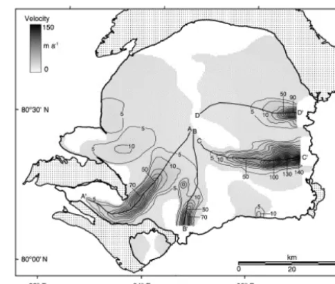
The observations were based on digital Landsat imagery and satellite InSAR and revealed four drainage basins and four fast-flowing ice streams on the southern side of the Academy of Sciences Ice Cap (Fig. 2; Dowdeswell et al., 2002). The four ice streams were 17–37 km long and 4–8 km wide (Dowdeswell et al., 2002). Bedrock elevations of these areas were below sea level, and the ice flow velocities

at-tained a value of 70–140 m a−1(Fig. 2). Such fast flow-line

features are typical for outlet glaciers and ice streams in both the Arctic and the Antarctic. These ice streams are the major locations of iceberg calving from the Academy of Sciences Ice Cap (Dowdeswell et al., 2002).

(2)

simu-Figure 1. After Dowdeswell et al., 2002, a map of Severnaya Zemlya showing the Academy of Sciences Ice Cap on Komsomo-lets Island, together with the other ice caps in the archipelago: Ru-sanov Ice Cap, Vavilov Ice Cap, Karpinsky Ice Cap, University Ice Cap, Pioneer Glacier, Semenov-Tyan-Shansky Glacier, Kropotkin Glacier, and Leningrad Glacier. The inset shows the location of Sev-ernaya Zemlya and the nearby Russian Arctic archipelagos of Franz Josef Land and Novaya Zemlya within the Eurasian High Arctic.

lated with a two-dimensional flow-line higher-order finite-difference model (e.g., Colinge and Blatter, 1998; Pattyn, 2000, 2002). This model describes an ice flow along a flow line (Pattyn, 2000, 2002). The results of diagnostic exper-iments undertaken by Konovalov (2012) show that for the

C–C0flow-line profile, the ice surface velocity along the flow

line attains a value of 100 m a−1, assuming that ice is sliding.

However, the observed surface velocity distribution along the

C–C0flow-line profile (Dowdeswell et al., 2002) is not

sim-ilar to that obtained by the model experiments for constant values of friction coefficients and for both linear and non-linear friction laws (Konovalov, 2012). Similarly, the

diag-nostic experiments conducted for the B–B0and D–D0profile

data show the same results for the ice flow velocities. The de-viation between the observed and modeled surface velocities suggests that the friction coefficients should be spatially vari-able. Therefore, to achieve a better agreement between the observed and simulated velocities, the spatial distribution of the friction coefficients needs to be optimized and an inverse problem needs to be solved (e.g., MacAyeal, 1992; Sergienko et al., 2008; Arthern and Gudmundsson, 2010; Gagliardini et al., 2010; Habermann et al., 2010; Morlighem et al., 2010;

Figure 2.After Dowdeswell et al., 2002, interferometrically cor-rected derived ice surface velocities for the Academy of Sciences Ice Cap. The first two contours are at velocities of 5 and 10 m a−1, with subsequent contours at 10 m a−1intervals. The unshaded areas of the ice cap are regions of uncorrected velocity data. The dotted areas represent bare land. The four fast-flowing ice stream central lines are denoted as A–A0, B–B0, C–C0, and D–D0. The velocity profiles of A–A0to D–D0 are shown in Fig. 11 of Dowdeswell et al. (2002).

Jay-Allemand et al., 2011; Larour et al., 2012; Sergienko and Hindmarsh, 2013).

The inversion of friction coefficients is based on the min-imization of the deviation between the observed and mod-eled surface velocities. A series of test experiments (Kono-valov, 2012), in which modeled surface velocities were used as observations in the inverse problem, have shown that the inverse problem for the full 2-D ice flow-line model is ill posed. More precisely, the surface velocity is weakly sensi-tive to small perturbations in the friction coefficient, and as a result the perturbations appear in the inverted friction coeffi-cients (Konovalov, 2012).

Herein, in a series of prognostic experiments we used the friction coefficient inversions obtained by applying Tikhonov’s regularization method, in which Tikhonov’s sta-bilizing functional is added to the main discrepancy func-tional (Tikhonov and Arsenin, 1977).

The inversions of the friction coefficients were used in the prognostic experiments for the fast-flowing ice streams. The 2-D prognostic experiments were numerical simulations with ice thickness distribution changes performed by the 2-D flow-line thermocoupled model, which includes (i) di-agnostic equations, (ii) the heat-transfer equation and (iii) the mass-balance equation (Pattyn, 2000, 2002). Here, we present the results of the prognostic experiments performed

for the B–B0, C–C0, and D–D0profiles (Fig. 3). Specifically,

(3)

0 10 20 30 40

Distance from the summit (m)

-200 0 200 400 600 800 E le va ti on ( m ) (a)

0 10 20 30 40

Distance from the summit (km)

-200 0 200 400 600 800 E le va ti on ( m ) (b)

0 10 20 30 40

-200 0 200 400 600 E le va ti on ( m ) (c)

Figure 3.(a)B–B0flow-line profile, which crosses downstream of one of the four fast-flowing ice streams in the Academy of Sciences Ice Cap (Fig. 2).(b)C–C0flow-line profile.(c)D–D0flow-line pro-file. The ice surface and ice bed elevation data were imported from Fig. 8 of Dowdeswell et al. (2002).

streams (Fig. 2) that are the main sources of the ice flux from the ice cap to the ocean. The results of the prognostic experi-ments include future modeled histories of ice thickness distri-butions along the flow lines of grounding-line locations and outgoing ice fluxes. The surface mass balance in the experi-ments was considered to be time-independent, and therefore the prognostic experiments revealed minimal ice mass loss in the ice streams in the future because the forecasts obtained did not account for future global warming. Nevertheless, the results of the prognostic experiments were in agreement with the observations of ice mass loss in the Severnaya Zemlya archipelago (Moholdt et al., 2012).

2 Field equations

2.1 Forward problem: diagnostic equations

The 2-D flow-line higher-order model includes the continu-ity equation for an incompressible medium, the mechanical equilibrium equation in terms of stress deviator components (Pattyn, 2000, 2002), and Glen’s flow law (Cuffey and Pater-son, 2010):                            z R hb ∂u ∂xdz

0 +1 b db dx z Z hb

udz0+w−wb=0,

2∂σ 0 xx ∂x + ∂σ0 yy ∂x + ∂2 ∂x2 hs Z z

σ0xzdz+

∂σ0xz

∂z =ρg

∂hs ∂x,

σ0ik=2ηε˙ik;η=

1

2(m A(T))

−1_n_˙

ε1−nn_, 0< x < L;h_b(x)< z < h_s(x),

(1)

where (xz) is a rectangular coordinate system with thexaxis

along the flow line and thezaxis pointing vertically upward;

uandw are the horizontal and vertical ice flow velocities,

respectively;b is the width along the flow line;σ0ik is the

stress deviator;ε˙ik is the strain-rate tensor;ε˙ is the second

invariant of the strain-rate tensor;ρ is the ice density;gis

the gravitational acceleration;ηis the ice effective viscosity;

A(T) is the flow-law rate factor; T is the ice temperature;

hb(x) andhs(x) are the ice bed and ice surface elevations,

respectively; andLis the glacier length.

The boundary conditions and some complementary exper-iments that were conducted by applying this model were con-sidered in Konovalov (2012). In particular, the technique in which the boundary conditions are included in the momen-tum equations in Konovalov (2012) was applied in the prog-nostic experiments considered here.

2.2 Inverse problem for the friction coefficient

The inversion of the friction coefficient was conducted us-ing the gradient minimization procedure for the smoothus-ing functional (Tikhonov and Arsenin, 1977):

F=

L

Z

0

(uobs−umod)2dx+β

L

Z

0

K_fr2+q(x)

dKf r dx

2!

dx, (2)

whereuobs is the observed velocity along the flow line and

umodis the modeled velocity. The first integral8is the

dis-crepancy, the second integralis the stabilizer (Tikhonov

and Arsenin, 1977),β is the regularization parameter, and

q(x) is considered equal to 1. The nonzero value ofβ

im-plies that the inverse problem, i.e., the problem that is based

on the minimization of the discrepancy8, is ill posed and the

(4)

in Nagornov et al. (2006) and Konovalov (2012). In this study the inversions were obtained for the linear (viscous) friction law based on the experiments implemented in

Kono-valov (2012), with inversions for the C–C0profile, in which

there was a good agreement between the observed (uobs) and

the calculated (umod) surface velocities for the linear friction

law.

2.3 Prognostic equations

The results of thermocoupled prognostic experiments imply that the 2-D flow-line model includes the heat-transfer equa-tion (Pattyn, 2000, 2002)

∂T ∂t =χ

_∂2_T

∂x2 +

1 b

db dx

∂T

∂x +

∂2T ∂z2

−

u∂T

∂x +w

∂T ∂z

+2A

−_n1_ε_˙1+_nn

ρC , (3)

whereχ andC are the thermal diffusivity and the specific

heat capacity, respectively. The terms in the first and in the second brackets define the heat transfer due to heat diffusion and ice advection, respectively. The last term is associated with strain heating.

In this model it is suggested that the ice surface tempera-ture at the Academy of Sciences Ice Cap varies with an el-evational gradient of temperature change, which is equal to

about 6.5◦C km−1. Hence, the ice surface temperature

dis-tribution along the flow line is defined by the temperature

history at the summitTs0(t) and by the elevational changes,

and is expressed as

Ts(x, t)=Ts0(t)+θT(hs(0)−hs(x)), (4)

whereθT is the elevational gradient. Therefore, Eq. (4)

pro-vides the boundary condition on the ice surface. However, it should be noted that Eq. (4) does not account for warming through the refreezing of meltwater.

The boundary condition at the ice base is defined by the geothermal heat flux and by heating due to the basal friction. It is expressed as (Pattyn, 2000, 2002)

∂T

∂z = −

1

k Q+ σ

0

xz_bub, (5)

wherekis the thermal conductivity.

The boundary conditions at the ice (ice shelf) terminus and at the ice shelf base are defined by sea water temperature,

which was considered to be−2◦C in this study.

The ice thickness temporal changes along the flow line are described by the mass-balance equation (Pattyn, 2000, 2002)

∂H

∂t =Ms−Mb− 1 b

∂(ubH)

∂x , (6)

whereuis the depth-averaged horizontal velocity,Msis the

annual surface mass balance, and Mb is the melting rate at

the ice base.

The mass-balance equation requires two boundary condi-tions at the summit and at the ice terminus. The first condition

at the ice cap summit implies that∂hs

∂x =0. The second

con-dition applied in the ice terminus originates from the fact that the ice thicknesses in the ice shelf along the flow line attains a constant value at the terminus.

2.4 Grounding-line evolution

In the model the grounding-line position is defined from the hydrostatic equilibrium (Schoof, 2007; Pattyn et al., 2012; Seroussi et al., 2014). Because sea water flow under the ice shelf is not considered in the model, and hence the pressure in Eqs. (10) and (11) from Pattyn et al. (2012) are equal to hydrostatic pressure, the grounding-line position is located where

−ρwhr=H ρ, (7)

wherehris the bedrock elevation andρwis the water density.

3 Results of the numerical experiments

3.1 Inversions for the friction coefficient

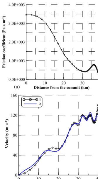
For the first run of the friction coefficient inversions, the linear ice temperature profile approximation was applied. Specifically, it was assumed that the ice temperature

lin-early increased from−15◦C at the surface to−5◦C at the

ice base at the division, and it increased from −2◦C to

−1◦C at the grounding line. Figure 4a shows the inverted

friction coefficient distribution along the C–C0 flow line.

The retrieved friction coefficient gradually decreased from

≈3.5×103Pa a m−1 _{to a mean value of 5}_×₁₀2_{Pa a m}−1

within a distance of around 25 km<×<40 km (Fig. 4a).

The difference between the simulated and observed surface velocities was relatively small (Fig. 4b) (Konovalov, 2012).

The inverted friction coefficient distributions along the B–

B0and D–D0flow lines had the same qualitative trends, i.e.,

they gradually decreased along the flow line from a higher to a lower level.

After the first run of the inversions, the ice temperature simulations were performed for inverted friction coefficients and boundary conditions (4) and (5). Boundary condition (4)

included the temperature historyTs0(t). In particular, if the

history was the past temperature (Nagornov et al., 2005, 2006), which was inverted previously from the borehole

tem-perature profile derived at the summit (80.50◦_{N, 94.83}◦_E)

(5)

0 10 20 30 40

0.0E+000 1.0E+003 2.0E+003 3.0E+003 4.0E+003

F

ri

ct

io

n

co

ef

fi

ci

en

t (

P

a

m

-1)

(a)

0 10 20 30 40

0 40 80 120 160

Velocity (m

a

-1)

1 2

(b)

Figure 4.(a)The friction coefficient distribution obtained in the inverse problem for the linear friction law and for the observed surface velocity distribution along the C–C0flow line (Konovalov, 2012).(b)The ice surface horizontal velocity distributions along the flow line: 1 – the observed surface velocity distribution, taken from Fig. 11 of Dowdeswell et al. (2002); 2 – the modeled surface ve-locity distribution, which corresponds to the reconstructed friction coefficient in Fig. 4a.

good agreement between the model results and the real phys-ical processes that occur in the glacier, which are generally described by the model. The past surface temperature his-tory, which was applied in the simulations of the present ice temperature, was adopted from Nagornov et al. (2005, 2006). The modeled present temperature distributions along the B–

B0, C–C0, and D–D0cross sections are shown in Fig. 5.

For the second run of the basal friction coefficient inver-sions, the modeled temperature distributions were applied (the modeled temperature was defined from Eqs. 3 to 5). The inverted friction coefficients for the (i) linearly approximated ice temperature and (ii) modeled ice temperature are shown in Fig. 6. Generally, the distinctions in the friction coeffi-cients were insignificant, and therefore the ice temperature approximations could be applied in the inverse problem as the first iteration of the ice temperature distribution in the glacier.

(

a)

(

b)

(

c)

Distance from the summit (m)

E

le

va

tio

n

(m

)

0 0.5 1 1.5 2 2.5 3 3.5 4

x 104 -100

0 100 200 300 400 500 600 700

-16 -14 -12 -10 -8 -6 -4 B-B' cross section

Distance from the summit (m)

E

le

va

tion

(m

)

0 0.5 1 1.5 2 2.5 3 3.5 4

x 104

-100 0 100 200 300 400 500 600

-16 -14 -12 -10 -8 -6 -4

C-C' cross section

Distance from the summit(m)

Elevation

(

m

)

0 0.5 1 1.5 2 2.5 3 3.5 4

x 104

-100 0 100 200 300 400 500

-16 -14 -12 -10 -8 -6 -4 -2 D-D' cross section

Figure 5.The temperature distributions within(a)the B–B0cross section,(b)C–C0 cross section, and(c)D–D0 cross section simu-lated by the model, with the past surface temperature history based on the paleotemperature, which was retrieved from the borehole temperature data (Nagornov et al., 2005, 2006).

3.2 Prognostic experiments

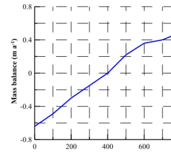
The main input data along with flow-line profiles for the prognostic experiments, namely, the surface mass balance, were adopted from Bassford et al. (2006). Figure 7 shows

the elevational mass-balance distribution along the C–C0_flow

line, i.e., it shows how the surface mass balance changes with

elevation in the C–C0direction (Bassford et al., 2006). For the

B–B0and D–D0flow lines, the elevational mass-balance

(6)

un-0 10 20 30 40 Distance from the summit (km) 0.0E+000

2.0E+003 4.0E+003 6.0E+003 8.0E+003 1.0E+004

F

ric

tio

n

c

oe

ff

ic

ie

nt

(

P

a

a m

-1)

1 2

0 10 20 30 40

Distance from the summit (km) 0.0E+000

1.0E+003 2.0E+003 3.0E+003 4.0E+003 5.0E+003

F

ri

cti

on

c

oe

ff

ic

ien

t (

P

a a

m

-1)

1 2

0 10 20 30 40

Distance from the summit (km) 0.0E+000

4.0E+003 8.0E+003 1.2E+004

F

ri

cti

on

c

oe

ffi

ci

en

t

(P

a a

m

-1)

1 2

(c)

(b)

(a)

Figure 6.The friction coefficients inverted along the(a)B–B0flow line,(b)C–C0flow line and(c)D–D0flow line. Curve 1 is the first inversion, which was obtained for the linear ice temperature profiles (the ice temperature approximation for the initial inversions). Curve 2 is the second inversion, which corresponds to the modeled ice temperature (Fig. 5).

der consideration. We intended to assess the maximum ice thickness in the ice streams in the future because the fore-casts implemented with the time-independent surface mass balance did not imply a future global warming and there-fore did not suggest a future decrease in surface mass

bal-0 200 400 600 800

Elevation (m)

-0.8 -0.4 0 0.4 0.8

Mass

balance

(m

a

-1)

Figure 7.The surface mass-balance elevational distribution along the C–C0flow line (Bassford et al., 2006).

ance Ms in Eq. (6). Similarly, the ice surface temperature

is suggested to be time-independent, but dependent on ele-vation, i.e., according to Eq. (4) it changes with eleele-vation,

with a constant value ofTs0(t). From the borehole

temper-ature measurements, the present ice surface tempertemper-ature at

the summit was about−7.2◦C. The initial ice temperatures

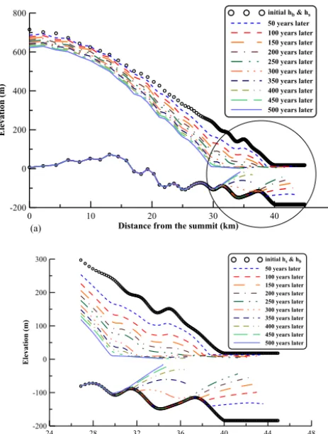
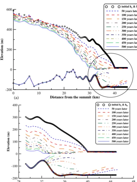
applied in the prognostic experiments are shown in Fig. 5. Despite future warming scenarios not being included in the prognostic experiments, the modeled ice cap response to the present environmental impact, which is reflected in the elevational mass-balance distribution (Bassford et al., 2006), revealed that the ice thickness gradually diminished along all three flow lines. Figures 8a–10a show the modeled suc-cessive ice surfaces divided into 50-year time intervals for

the B–B0, C–C0, and D–D0profiles, respectively. Figures 8b–

10b show the same results as Figs. 8a–10a, respectively, but these complementary figures show the evolution of the three ice shelves in more detail. The prognostic experiments were performed by applying a rectangular ice shelf geometry. The cumulative impact of sea water, surface mass balance, and ice flow changes in the glacier produced the future modeled ice shelf geometries. The ancillary black circles in Figs. 8a, b to 10a, b are aligned with the grid nodes; thus, they show the spatial resolution at which the prognostic experiments were implemented. The spatial resolution was irregular and

decreased from about 2×103m at the summit to about 102m

in the grounding-line vicinity and in the ice shelf. The spatial grid was considered unchangeable throughout the period of the modeling.

The grounding-line history, i.e., grounding-line retreat or advance, specifically reflects a growing or diminishing ice mass, i.e., its history is an indicator of glacier evolution. The

grounding line retreated (a) along the B–B0 flow line from

≈40 to≈30 km (Fig. 11a), (b) along the C–C0 flow line

from≈43 to ≈37 km (Fig. 11b), and (c) along the D–D0

flow line from≈41 to≈32 km (Fig. 11c) over a time period

(7)

0 10 20 30 40 50

-200 0 200 400 600 800

El

ev

at

ion

(

m

)

initial hb & hs

50 years later 100 years later 150 years later 200 years later 250 years later 300 years later 350 years later 400 years later 450 years later 500 years later

(a)

24 28 32 36 40 44 48

-200 -100 0 100 200 300

E

le

vat

io

n

(

m

)

initial hs & hb 50 years later 100 years later 150 years later 200 years later 250 years later 300 years later 350 years later 400 years later 450 years later 500 years later

(b)

Figure 8.(a)The modeled successive B–B0cross-section geome-tries separated by 50-year intervals from the present to 500 years later.(b)A magnified section of panel(a), showing the evolution of the B–B0ice shelf.

The results of the prognostic experiments can be treated in the same way, suggesting changes in the friction coeffi-cients. The glacier terminus, which is currently fast flowing and therefore experiencing pressure melting, eventually be-came frozen to the ground. The ice thickness was insufficient to provide insulation from the cold atmosphere and reduced driving stress and strain heating. Therefore, the basal fric-tion coefficients could change drastically, given the simulated changes in glacier geometry.

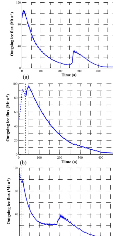
The ice flow velocities in the ice streams decrease with time and this trend diminishes the outgoing ice fluxes in the future. Figure 12 shows the modeled outgoing ice flux

histo-ries, i.e., it shows how the valueubH, which is defined at the

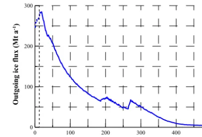
ice shelf terminus, changes with time. Accordingly, Fig. 13 shows the future history of the overall outgoing ice flux, i.e., it is the sum of the three future modeled historical trends that are shown in Fig. 12.

There are small peaks that periodically disturb the main historical trends of the three outgoing ice fluxes. Each peak reflects ice calving at the ice shelf terminus. Similarly, the ice calving represents a sudden change in the value of the

outgoing ice flux (ubH) due to a sudden change in the ice

0 10 20 30 40 50

-200 0 200 400 600 800

E

le

va

ti

on

(m

)

initial hs & hb

(a)

32 36 40 44 48

-200 -100 0 100 200 300

El

ev

at

ion

(m

)

initial hs & hb 50 years later 100 years later 150 years later 200 years later 250 years later 300 years later 350 years later 400 years later 450 years later 500 years later

(b)

Figure 9.(a)The modeled successive C–C0cross-section geome-tries separated by 50-year intervals from the present to 500 years later.(b)A magnified section of panel(a), showing the evolution of the C–C0ice shelf.

thickness (H) at the terminus. Considering the complex

en-vironmental impact on ice shelves (Bassis et al., 2008), from the mathematical perspective it can be suggested that at long timescales the calving processes are described by a stochastic model, which considers the size of the anticipated ice debris as a random value. This value satisfies a probability distribu-tion law, similar to the Gaussian distribudistribu-tion for example. In the model, we considered the simplest probability distribu-tion, i.e., when debris of equal length occurred at each calv-ing. Thus, the length of ice debris was the parameter that cor-responded to the average length in a probability distribution law (for example in the Gaussian distribution).

In this model, both the ice shelf length and ice shelf thick-ness at the terminus were considered to be variables that could satisfy certain conditions. If the ice shelf length

ex-ceeded a valuelcr(the parameter of the model) or the ice shelf

thickness beside the terminus became smaller than a value

Hcr, then the calving of the appropriate part of ice would

oc-cur in the model.

(8)

0 10 20 30 40 50

-200 0 200 400 600

El

ev

a

ti

o

n

(m

)

initial hs & hb

(a)

28 32 36 40 44 48

-200 -100 0 100 200 300 400

E

le

v

a

ti

on

(m

)

initial hs & hb

(b)

Figure 10.(a)The modeled successive D–D0cross-section geome-tries separated by 50-year intervals from the present to 500 years later.(b)A magnified section of panel(a), showing the evolution of the D–D0ice shelf.

ice temperature had the main impact on the assessment of the grounding-line retreat derived by the modeling.

4 Discussion

Numerical experiments conducted with a 2-D model using the randomly perturbed friction coefficient have revealed that the horizontal surface velocity is weakly sensitive to the per-turbations (Fig. 4 of Konovalov, 2012). Thus, the

perturba-tions appear on thex-distributed inverted friction coefficient.

Therefore, the inverse problem should be considered as ill posed because the weak sensitivity of the surface velocity to the perturbations in the friction coefficient justifies the in-stability in the inverse problem. In other words, the instabil-ity in the inverse problem means that small deviations in the observed surface velocities allow significant perturbations in the friction coefficient. Hence, the application of the regular-ization method is justified.

Tikhonov’s method is based on the application of the sta-bilizing functional, which proportionally reduces the effects

of perturbations of the regularization parameterβ(Tikhonov

and Arsenin, 1977). A further increase in the parameter leads

to a reduction in the real spatial variability of the friction co-efficients.

The reduction in the existing friction coefficient variabil-ity is associated with a growing discrepancy between the ob-served and modeled surface velocities. Thus, the regulariza-tion parameter is chosen as the value at which nonexistent perturbations are reduced, but the real variability of the fric-tion coefficient is not completely reduced by the stabilizing functional. The optimal value of the regularization parameter can be defined approximately in the curve, which is the devi-ation between the observed and modeled surface velocities versus the regularization parameter (Leonov, 1994; Kono-valov, 2012).

Evidently, the stabilizing functional narrows down the

range of possible invertedxdistributions of the friction

coef-ficients. Thus, it is assumed a priori that the real spatial

distri-bution of the friction coefficient with respect to thexaxis is

a smooth function. Moreover, the friction coefficient in the friction laws is considered to be a constant (e.g., Van der Veen, 1987; MacAyeal, 1989; Pattyn, 2000; Gudmundsson, 2011). Hence, the friction coefficient inversion performed for the three cross sections can be interpreted as follows.

The two evidently distinguished levels in the inverted fric-tion coefficient distribufric-tions can be explained by chang-ing the physical properties of the bedrock along the flow lines. Similarly, the large values of the friction coefficient at km< x <20 km justify the bedrock (more likely, marine sed-iments; Dowdeswell et al., 2002) where ice is frozen to the

bed (the ice temperature at km< x <20 km is lower than the

melting point). The lower values of the friction coefficient

at 25 km< x <40 km presumably indicate the existence of a

water-saturated till layer at the bottom (e.g., Engelhardt et al., 1978, 1979; Boulton, 1979; Boulton and Jones, 1979; MacAyeal, 1989; Engelhardt and Kamb, 1998; Iverson et al., 1998; Tulaczyk et al., 2000). Specifically, the till layer (de-formable basal sediments) enables the basal ice sliding.

The modeled ice temperatures at present (Fig. 5) were qualitatively the same in the three cross sections. There were resembling zones of relatively cold ice that could be distin-guished in the modeled temperatures approximately in the middle (in the vertical dimension) of each cross section. These cold ice zones reflected the surface temperature min-imum about 150–200 years ago in the inverted past tem-perature history (Nagornov et al., 2005, 2006). This surface temperature minimum corresponds to an event known as the Little Ice Age. Thus, surface boundary conditions (4), and diffusive and advective heat transfers were responsible for the basal ice temperature, which was mainly in the range

of−9 to−4◦C at 25 km< x <40 km. Therefore, the

(9)

0 100 200 300 400 500 Time (a)

28 32 36 40

G

ro

u

n

d

in

g

-l

in

e

p

o

si

ti

o

n

(

k

m

)

(a)

0 100 200 300 400 500

Time (a) 36

38 40 42 44

G

ro

u

n

d

in

g

-l

in

e

p

o

si

ti

o

n

(

k

m

)

(b)

0 100 200 300 400 500

Time (a) 32

34 36 38 40 42

G

ro

u

n

d

in

g

-l

in

e

p

o

si

ti

o

n

(

k

m

)

(c)

Figure 11.The modeled grounding-line history for the(a)B–B0 cross section(b)C–C0and(c)D–D0cross section.

However, note that the heat-transfer model considered here does not account for meltwater refreezing in the subsur-face firn layer (Paterson and Clarke, 1978). The numerical experiments undertaken by Paterson and Clarke (1978) re-vealed that the heat source had a significant impact on the ice temperature profiles due to melt water refreezing, depend-ing on its percolation depth. Thus, the notion that the basal ice temperature is higher than the modeled temperature and could reach the melting point cannot be dismissed.

General formulations of the friction laws assume that the appropriate equations include the effective basal pressure (e.g., Budd et al., 1979; Iken, 1981; Bindschadler, 1983; Jansson, 1995; Pattyn, 2000; Vieli et al., 2001). Introduction of the effective pressure in Eq. (2) does not provide a

con-0 100 200 300 400 500

Time (a)

0 40 80 120

Outgoing

ice

flux

(Mt

a

-1)

(a)

0 100 200 300 400 500

Time (a) 0

20 40 60 80 100

Outgoing

ice flux (Mt

a

-1)

(b)

0 100 200 300 400 500

Time (a) 0

40 80 120

Outgoing

ice flux (Mt

a

-1)

(c)

Figure 12.The modeled outgoing ice flux history for the(a)B–B0, (b)C–C0, and(c)D–D0cross sections.

stant value of the inverted friction coefficient atx >25 km.

The inversion performed for the nonlinear Weertman-type friction law (Weertman, 1957) reveals similar variations in

the inverted friction coefficient at x >25 km (Konovalov,

(10)

eleva-tion changes, and the enhancement of water content at lower elevations provides a decrease in the friction coefficient in the corresponding areas.

Finally, two areas were identified in the bedrock, where

basal ice was frozen to the bed (km< x <20 km) and where

basal sliding occurred (25 km< x <40 km) due to the till

layer. The boundary of the transition from the area of the frozen basal ice to the area of the basal sliding was diluted due to smoothing of the inverted friction coefficient by the stabilizer. The linear friction law provided a good agreement between the observed and modeled surface velocity distri-butions along the flow line. Thus, it could be conveniently applied in these applications (in particular, in the prognostic experiments).

The prognostic experiments reveal that the extent of both ice mass and ice stream declined with respect to the refer-ence time-independent mass balance (Bassford et al., 2006). These experiments demonstrated that the grounding lines would retreat by about 10 km for the three ice streams over a time period of 500 years and with a steady-state environmen-tal impact, i.e., a constant elevation-dependent surface mass balance. The ice flow velocities in the ice streams would decrease with time due to (a) a diminishing of ice thick-nesses (and thus decreasing driving stress) and (b) a retreat of the grounding lines from the sliding zones toward the zones where ice is frozen to the bed (inverted friction coefficient distributions are considered to be time-independent). Thus, the maxima of the ice flow velocities in the ice streams

de-creased from 80− −120 to 20− −30 m a−1. These trends

in the ice flow velocities reduced the outgoing ice fluxes (Fig. 12) and as a result diminished the overall ice flux (Fig. 13).

Observations in the Russian High Arctic (Moholdt et al., 2012) have revealed that over the period between Oc-tober 2003 and OcOc-tober 2009 the archipelagos of Franz Josef Land and Novaya Zemlya have lost ice at a rate of

−9.1±2.0 Gt a−1. Over this period the ice loss from

Sever-naya Zemlya was evaluated as being−1.4±0.9 Gt a−1

(Mo-holdt et al., 2012). The modeling shows that other than this period the Academy of Sciences Ice Cap (the largest of the 10 glaciers located on Severnaya Zemlya) could lose about

0.2 to 0.3 Gt a−1(Fig. 13).

5 Conclusions

The modeled ice temperatures at present (Fig. 5) are qualita-tively the same in the three cross sections. There are resem-bling zones of relatively cold ice that can be distinguished in the modeled temperatures in the middle of the cross sec-tions. These cold ice zones reflected the surface temperature minimum about 150–200 years ago in the inverted past tem-perature history (Nagornov et al., 2005, 2006). This surface temperature minimum corresponds to the event known as the Little Ice Age.

0 100 200 300 400 500

Time (a) 0

100 200 300

Outgoing

ice

flux

(Mt

a

-1)

Figure 13.The overall outgoing ice flux history (the sum of the outgoing fluxes for the three ice streams: B–B0, C–C0, and D–D0).

The inversions of the friction coefficient performed for the three cross sections can be interpreted as follows. The two levels that are evidently distinguished in the inverted friction coefficient distributions (Fig. 6) can be explained by chang-ing the physical properties of the bedrock along the flow lines. Similarly, the large values of the friction coefficient at km< x <20 km justify the bedrock where ice is frozen to the

bed (the ice temperature at km< x <20 km is lower than the

melting point). The lower values of the friction coefficient

at 25 km< x <40 km presumably indicate the existence of a

till layer at the bottom. Specifically, the till layer enables the basal ice sliding.

The prognostic experiments conducted with the reference mass balance (Bassford et al., 2006) show that the ground-ing line would retreat by about 10 km in the three ice streams over a time period of 500 years. Similarly, the grounding line

would retreat (a) along the B–B0 flow line from≈40 km to

≈30 km (the distance from the summit), (b) along the C–

C0 flow line from ≈43 km to ≈37 km, and (c) along the

D–D0 flow line from≈41 to ≈32 km over a time period

of 500 years, assuming a time-independent mass balance. In the experiments, the ice flow velocities in the ice streams de-creased with time due to (a) diminishing of the ice thick-nesses and (b) retreat of the grounding lines from the sliding zones toward the zones where ice is frozen to the bed. Thus, the maxima of the ice flow velocities in the ice streams

de-creased from 80− −120 to 20− −30 m a−1. These trends in

the ice flow velocities reduced the outgoing ice fluxes and as a result diminished the overall ice flux (Fig. 13). The mod-eled evolution of the ice streams is in agreement with obser-vations of ice mass loss in the Severnaya Zemlya archipelago (Moholdt et al., 2012).

(11)

Competing interests. The authors declare that they have no con-flict of interest.

Acknowledgements. The authors are grateful to J. A. Dowdeswell et al. for the data that have been used in the paper. The authors are grateful to F. Pattyn for the useful comments made regarding the paper. The authors are grateful to T. Dunse and the anonymous referees for reviewing the paper.

Edited by: V. Lucarini

Reviewed by: T. Dunse and one anonymous referee

References

Arkhipov S. M.: Data Bank “Deep drilling of glaciers: Soviet-Russian Projects in Arctic, 1975–1990”, Data of Glaciological Studies, 87, 229–238, 1999.

Arthern, R. and Gudmundsson, H.: Initialization of ice-sheet fore-casts viewed as an inverse Robin problem, J. Glaciol, 56, 527– 533, 2010.

Bassford, R. P., Siegert, M. J., and Dowdeswell, J. A.: Quantify-ing the Mass Balance of Ice Caps on Severnaya Zemlya, Rus-sian High Arctic III: Sensitivity of Ice Caps in Severnaya Zemlya to Future Climate Change, Arct. Antarct. Alp. Res., 38, 31–33, available at: http://www.jstor.org/stable/4095823, 2006. Bassis, J. N., Fricker, H. A., Coleman, R., and Minster, J.-B.: An

investigation into the forces that drive ice-shelf rift propagation on the Amery Ice Shelf, East Antarctica, J. Glaciol., 54, 17–27, 2008.

Bindschadler, R.: The importance of pressurized subglacial water in separation and sliding at the glacier bed, J. Glaciol., 29, 3–19, 1983.

Boulton, G. S.: Processes of glacier erosion on different substrata, J. Glaciol., 23, 15-38, 1979.

Boulton, G. S. and Jones, A. S.: Stability of temperate ice caps and ice sheets resting on beds of deformable sediment, J. Glaciol., 24, 29–43, 1979.

Budd, W. E., Keage, P. L., and Blundy, N. A.: Empirical studies of ice sliding, J. Glaciol., 23, 157–170, 1979.

Colinge J. and Blatter, H.: Stress and velocity fields in glaciers: Part I. Finite difference schemes for higher-order glacier models, J. Glaciol., 44, 448–456, 1998.

Cuffey, K. and Paterson, W. S. B.: The physics of glaciers, 4th Edn., Butterworth-Heinemann, Elsevier, Oxford, UK, 2010.

Dowdeswell, J. A., Bassford, R. P., Gorman, M. R., Williams, M., Glazovsky, A. F., Macheret, Y. Y., Shepherd, A. P., Vasilenko, Y. V., Savatyugin, L. M., Hubberten, H. W., and Miller, H.: Form and flow of the Academy of Sciences Ice Cap, Sever-naya Zemlya, Russian High Arctic, J. Geophys. Res., 107, 1–15, doi:10.1029/2000JB000129, 2002.

Engelhardt, H. and Kamb, B.: Basal sliding of Ice Stream B, West Antarctica, J. Glaciol., 44, 223–230, 1998.

Engelhardt, H. F., Harrison, W. D., and Kamb, B.: Basal sliding and conditions at the glacier bed as revealed by bore-hole photogra-phy, J. Glaciol., 20, 469–508, 1978.

Engelhardt, H. F., Kamb, B., Raymond, C. F., and Harrison, W. D.: Observation of basal sliding of Variegated Glacier, Alaska, J. Glaciol., 23, 406–407, 1979.

Gagliardini O., Jay-Allemand, M., and Gillet-Chaulet, F.: Friction distribution at the base of a surging glacier inferred from an in-verse method, San Francisco, CA, USA, AGU Fall Meeting, 13– 17 December, Abstract: C13A-0540, 2010.

Gudmundsson, G. H.: Ice-stream response to ocean tides and the form of the basal sliding law, The Cryosphere, 5, 259–270, doi:10.5194/tc-5-259-2011, 2011.

Habermann, M., Maxwell, D. A., and Truffer, M.: A principled stopping criterion for the reconstruction of basal properties in ice sheets, San Francisco, CA, USA, AGU Fall Meeting, December 13-17, Abstract: C21C-0556, 2010.

Hewitt, I. J.: Modelling distributed and channelized subglacial drainage. The spacing of channels, J. Glaciol., 57, 302–314, doi:10.3189/002214311796405951, 2011.

Hoffman, M. and Price, S.: Feedbacks between coupled subglacial hydrology and glacier dynamics, J. Geophys. Res-Earth, 119, 414–436, doi:10.1002/2013JF002943, 2014.

Iken, A.: The effect of the subglacial water pressure on the sliding velocity of a glacier in an idealized numerical model, J. Glaciol., 27, 407–421, 1981.

Iverson, N. R., Hooyer, T. S., and Baker, R. W.: Ring-shear stud-ies of till deformation: Coulomb-plastic behavior and distributed strain in glacier beds, J. Glaciol., 44, 634–642, 1998.

Jansson, P.: Water pressure and basal sliding on Storglaciären, northern Sweden, J. Glaciol., 41, 232–240, 1995.

Jay-Allemand, M., Gillet-Chaulet, F., Gagliardini, O., and Nodet, M.: Investigating changes in basal conditions of Variegated Glacier prior to and during its 1982–1983 surge, The Cryosphere, 5, 659–672, doi:10.5194/tc-5-659-2011, 2011.

Knight, P. G.: Glaciers, Stanley Thornes Ltd., Cheltenham, UK, 1999.

Konovalov, Y. V.: Inversion for basal friction coefficients with a two-dimensional flow line model using Tikhonov regularization, Res. Geophys., 2, 82–89, 2012.

Larour, E., Seroussi, H., Morlighem, M., and Rignot, E.: Continen-tal scale, high order, high spatial resolution, ice sheet modeling using the Ice Sheet System Model (ISSM), J. Geophys. Res., 117, 1–20, 2012.

Leonov, A. S.: Some a posteriori termination rules for the itera-tive solution of linear ill-posed problems, Comput. Math. Math. Phys., 34, 121–126, 1994.

MacAyeal, D. R.: Large-scale ice flow over a viscous basal sedi-ment: theory and application to ice stream B, Antarctica, J. Geo-phys. Res., 94, 4071–4088, 1989.

MacAyeal, D. R.: The basal stress-distribution of Ice Stream-E, Antarctica, inferred by control methods, J. Geophys. Res.-Sol. Ea., 97, 595–603, 1992.

Moholdt, G., Wouters, B., and Gardner, A. S.: Recent mass changes of glaciers in the Russian High Arctic, Geophys. Res. Lett., 39, L10502, doi:10.1029/2012GL051466, 2012.

(12)

Nagornov, O. V., Konovalov, Y. V., and Tchijov, V.: Reconstruction of past temperatures for Arctic glaciers subjected to intense sub-surface melting, Ann. Glaciol., 40, 61–66, 2005.

Nagornov, O. V., Konovalov, Y. V., and Tchijov, V.: Temperature reconstruction for Arctic glaciers, Palaeogeogr. Palaeocl., 236, 125–134, 2006.

Nye, J. F.: Water flow in glaciers: jökulhlaups, tunnels and veins, J. Glaciol., 17, 181–207, 1976.

Paterson, W. S. B. and Clarke, G. K. S.: Comparison of theoreti-cal and observed temperatures profiles in Devon Island ice cap, Canada, Geophys. J. Roy. Astr. S., 55, 615–632, 1978.

Pattyn, F.: Ice-sheet modeling at different spatial resolutions: focus on the grounding zone, Ann. Glaciol., 31, 211–216, 2000. Pattyn, F.: Transient glacier response with a higher-order numerical

ice-flow model, J. Glaciol., 48, 467–477, 2002.

Pattyn, F., Schoof, C., Perichon, L., Hindmarsh, R. C. A., Bueler, E., de Fleurian, B., Durand, G., Gagliardini, O., Gladstone, R., Goldberg, D., Gudmundsson, G. H., Huybrechts, P., Lee, V., Nick, F. M., Payne, A. J., Pollard, D., Rybak, O., Saito, F., and Vieli, A.: Results of the Marine Ice Sheet Model Intercomparison Project, MISMIP, The Cryosphere, 6, 573–588, doi:10.5194/tc-6-573-2012, 2012.

Röthlisberger, H.: Water pressure in intra- and subglacial channels, J. Glaciol., 11, 77–203, 1972.

Schoof, C.: Ice sheet grounding line dynamics: Steady states, stability, and hysteresis, J. Geophys. Res., 112, 1–19, doi:10.1029/2006JF000664, 2007.

Sergienko, O. V. and Hindmarsh, R. C. A.: Regular patterns in fric-tional resistance of ice-stream beds seen by surface data inver-sion, Science, 342, 1086–1089, 2013.

Sergienko, O. V., Bindschadler, R. A., Vornberger, P. L., and MacAyeal, D. R.: Ice stream basal conditions from block-wise surface data inversion and simple regression models of ice stream flow: Application to Bindschadler Ice Stream, J. Geophys. Res., 113, 1–11, 2008.

Seroussi, H., Morlighem, M., Larour, E., Rignot, E., and Khazen-dar, A.: Hydrostatic grounding line parameterization in ice sheet models, The Cryosphere, 8, 2075–2087, doi:10.5194/tc-8-2075-2014, 2014.

Tikhonov, A. N. and Arsenin, V. Y.: Solutions of ill-posed problems, Winston & Sons, Washington, 1977.

Tulaczyk, S., Kamb, W. B., and Engelhardt, H. F.: Basal mechanics of Ice Stream B, West Antarctica I. Till mechanics, J. Geophys. Res., 105, 463–482, doi:10.1029/1999JB900329, 2000. Van der Veen, C. J.: Longitudinal stresses and basal sliding: a

com-parative study, in: Dynamics of the West Antarctic ice sheet, edited by: Van der Veen, C. J. and Oerlemans J., D. Reidel Pub-lishing Co., Dordrecht, 223–248, 1987.

Vieli, A., Funk, M., and Blatter, H.: Flow dynamics of tidewater glaciers: a numerical modelling approach, J. Glaciol., 47, 595– 606, 2001.